Full Length Research Paper
Technical efficiency changes at the farm-level: A panel
data analysis of rice farms in Bangladesh
Mohammad Jahangir Alam
1,2*, Guido Van Huylenbroeck
1, Jeroen Buysse
1, Ismat Ara Begum
3,
and Sanzidur Rahman
41
Department of Agricultural Economics, Ghent University, 653 Coupure Links, 9000 Ghent, Belgium.
2
Department of Agribusiness and Marketing, Bangladesh Agricultural University, Mymensingh-2202, Bangladesh.
3
Department of Agricultural Economics, Bangladesh Agricultural University, Mymensingh-2202, Bangladesh.
4
School of Geography, Earth and Environmental Sciences, the University of Plymouth, Plymouth, PL4 8AA, UK.
Accepted 17 May, 2011
This paper examines technical efficiency changes at the farm-level for rice farms in Bangladesh over a 17 year period (1987 to 2004) using nationally representative panel data. Results from the stochastic production frontier analysis indicate that technical efficiency of the rice farmers has declined from 83% to 60% over this period due to a host of farm as well as socio-economic factors. Age, education, tenure status and involvement in off-farm work are factor negatively influencing technical efficiency while the relationship with farm size is positive. Under the current production technology and input use, 40% higher production could be reached by removing technical efficiency which is substantial. Policy recommendations include consolidation of land and strengthening of extension services.
Key words: Technical efficiency, rice farms, efficiency elasticity, panel data, Bangladesh.
INTRODUCTION
Rice is the staple food for the population of Bangladesh. The per capita rice consumption in Bangladesh is 441 g/day and more than 70% of total calorie intake comes from rice (Kenny, 2001). Rice contributes for 60% of the agricultural gross domestic production (GDP) which in turn accounts for about a third of the national GDP (BBS, 2009). As one of the most densely populated countries of the world, with a population already 140 million due to top population growth Bangladesh needs to feed an extra two million people every year (BBS, 2009). So, the central focus of agricultural policy and development efforts in Bangladesh is focused on increasing rice production maintaining food security and becoming self sufficient. However, although various policies have been under-taken since its independence in 1971 but success in realizing such an ambitious target remains elusive as the
*Corresponding author. E-mail: [email protected], [email protected]. Tel: 32 (9) 264 93 75. Fax: 32 (9) 264 62 46.
the country is still identified as one of the food deficit countries of the world. Although overall rice production steadily increased over the time, over-all food-security and self sufficiency is far from being achieved.
There is a consensus in the research arena and in the policy forum that long-term food security could be achieved by promoting productivity and output growth in the agricultural sector, particularly the rice sector. Many researchers (Hayami and Ruttan, 1985; Kuznets, 1966) advocate the adoption of new technologies to increase farm productivity. However, after observing the results of the green revolution in developing countries across the world, researchers and policy makers argue that productivity gains could also be possible by efficient use of the existing technology rather than introducing new technology (Bravo-Ureta and Pinheiro, 1997; Squires and Tabor, 1991) which may take a longer time from invention to adoption at the farm level.
It is imperative that the productivity of rice farmers in Bangladesh can be raised either by the adoption of improved production technologies or improvements in
efficiency or reconciling both. Therefore, technological progress in rice cultivation is crucial for sustaining food production and food security in Bangladesh. Although, Bangladesh has made remarkable progress in sustaining a positive growth in rice production over the last three decades through the adoption of high yielding modern varieties (MVs) of rice (Hossain et al., 2006), the yield per hectare remains much lower than in the other major rice producing countries in Asia. For example in 2000, average paddy production per hectare was 6800 kg in Korea republic, 6582 kg in Japan, 6300 kg in China, 4300 kg in Indonesia, and only 3465 kg in Bangladesh (FAO, 2009). As expansion and adoption rate of modern rice technologies by the farmers in Bangladesh is reaching its ceiling level (Baffes and Gautam, 2001), improvement in efficiency is probably the best and maybe only option in enhancing productivity. Many studies were conducted on estimating efficiency of farms in developing countries applying either the parametric stochastic frontier approach (SFA) or the non-parametric data envelopment analysis (DEA). Thiam et al. (2001) summarizes 51 studies on technical efficiencies in developing countries from all over the world. In Bangladesh, there are only a few studies that estimated efficiency at the farm-level (Salim and Hossain, 2006; Rahman, 2007; Wadud and White, 2000; Sharif and Dar, 1996). All these studies use only cross-sectional data. To our knowledge, no studies investigated technical efficiency (TE) of rice farmers at the farm-level in Bangladesh over time using a nationally representative panel data set, although regional level panel-data were utilized by Coelli et al. (2003) and Rahman (2007). Our main contribution to the existing literature is to fill this gap in knowledge by estimating and trying to explain the changes over time in production performance at the farm-level. The main objective of this paper is thus to identify the changes in farm-level tech-nical efficiency over time for rice farms in Bangladesh, which is the key sector to sustain agricultural growth of the economy. Next it also examines the factors that affect farm-level technical efficiency. In this paper we apply a stochastic frontier production function model, in which the technical efficiencies of farms are allowed to vary over time.
THEORETICAL STOCHASTIC FRONTIER MODEL The stochastic frontier approach (SFA) was for the first time independently proposed by Aigner et al. (1977) and Meeusen and Van den Broeck (1977). SFA has contri-buted significantly to the literature by using econometric modeling of production and technical efficiency of farms both in a static or a dynamic framework. SFA involves two random components, one associated with the presence of technical inefficiency and the other being a conventional random error. The advantage of the SFA is its capability to measure the efficiency in the presence of
statistical noise. Applications of frontier functions have involved both cross-sectional and panel data. In our study we use a panel data set as it is more informative and is able to capture dynamic behavior (Baltagi and Song, 2006). Specifically there are some advantages in using panel data instead of a cross section or time-series data (Hsiao, 2003 and Baltagi, 2005). These are: (1) Panel data have more variability and less collinearity among variables, (2) panel data controls individual heterogeneity and, therefore, able to get unbiased estimates and (3) able to identify and estimate effects which are not detectable in a cross-section or a time-series data. The SFA approach can effectively handle statistical noise in panel data but is adversely affected by measurement error when applied to cross-sectional data. Furthermore, Sickles (2005) and Gong and Sickles (1992) showed that the panel data version of the stochastic frontier model works well. This is because the panel data model incorporates additional information from the times-series nature of the data as well as the distributional assump-tions, which allow estimation via the method of maximum likelihood (ML). A panel data stochastic frontier model also has advantages over DEA (data envelopment analysis), which typically relies on cross-sectional data to estimate efficiency (Ruggiero, 2007). Therefore, we choose to apply SFA with a simple exponential specification of time-varying farm effects using a balanced panel of 73 farms over T (1987, 2000 and 2004) periods to estimate efficiency.
The stochastic frontier production function with a simple exponential specification of time varying farm effects can be defined as following Equation (1):
) exp( ) : ( it it it it f X V U Y =
β
− (1){
}
i i it it U t T U U =η
= exp[−η
( − )]t
∈
I
(
i
);
i
=
1
,
2
,...
.,
N
;
where the dependent variable Yit represents total rice
production (kg/farm) by the i-th farm in the t-th time period,
Xit denotes n-th factor inputs associated with the
production of the i-th farm in the t-th year, β is the vector of
unknown parameters to be estimated; the statistical noise Vit are assumed to be identically and independently
distributed (i.i.d) {N (0, σv 2
)} random errors. The other error components Uits are assumed to be i.i.d
non-negative random variables truncated at zero. The values of Uit range between zero and one, where 1 indicates full
technical efficiency and 0 indicates full technical inefficiency. In this model the time trend (t) also interacts with the inputs (land, seed, fertilizer labour and pesti-cides) which allows for non-neutral technical change. We also include time squared variable in this model which allows for non-monotonic technological change, η is an unknown scalar parameter, I (i) corresponds to the set set of Ti time periods among the T periods involved for
which observations for i-th farm are obtained. The model
followed the structure of Battese and Coelli (1992). The technical efficiency of an individual farmer is defined as the ratio of the observed output to the corresponding frontier output given the available
technology. The minimum mean squared error predictor of the technical efficiency of the i-th farm at the t-th time
period TEit = exp (-Uit) can be calculated by using
Equation (2):
+
−
−
Φ
−
−
Φ
−
=
−
2 1 2 1 * 1 * 1 * 1 * 1 * 1 * *2
1
exp
1
(
1
]
)
[exp(
η
µ
η
µ
σ
µ
σ
µ
µ
η
it it it i itE
U
E
(2) Where 2 2 2 1 2 1 *σ
η
η
σ
σ
η
µσ
µ
i i V i VE
′
+
′
−
=
and 2 2 2 2 *2σ
η
η
σ
σ
σ
σ
i i V V i′
+
=
Ei stand for the (
T
ix 1) vector ofE
it’ s correlated with thetime periods observed for the i-th farm, where
it it it
V
U
E
=
−
;η
itrepresents the (T
ix 1) vector ofn
itassociated with the time periods observed for the i-th
farm; and
Φ
(.) represents the distribution function for the standard normal random variable.However,
U
itcould decrease, remain constant orincrease as t increases, if η > 0, η= 0 or η < 0, respectively. The case in which η is positive is likely to be appropriate when farms tend to improve their level of technical efficiency over time and a negative value for η
means that the level of technical efficiency declines over time.
PANEL DATA
The data for this analysis are drawn from a repeated survey of a nationally representative sample of rural households. The 1987– 1988 Survey was conducted by the Bangladesh Institute of Development Studies (BIDS) on 1240 rural households from 62 villages of 57 out of 64 total districts in Bangladesh for a research on technological progress (Hossain et al., 1994; David and Otsuka, 1994). The representative sample was drawn by using a multistage
random sampling method. First, 64 unions (small administrative unit) were randomly selected from a list of all unions in the country, and then one village was selected from each union. A random sample of 20 households was drawn from each village. The 1999 to 2000 survey was conducted by the IRRI from the same villages for a research on poverty dynamics. A sample of 30 to 31 households from each of the 62 villages (1880 households) was drawn using stratified random sampling. The 2004 - 2005 survey was also conducted by IRRI and covered the same households as in the first two surveys of 1987 to 1988 and 2000 to 2001. In the 2004 to 2005 survey, the total sample size rose to 1927. The sample of these three surveys is nationally representative as documented by Hossain et al., 1994; Rahman and Hossain 1995.
However, because of the objective of our paper, we need to use farm level panel data. Therefore, we consolidated the same farm households who are present in all three surveys so that we get a balanced panel for a cohort of 73 farm households. The total observation stands at 219 and covers 26 administrative districts, thereby making our data-set nationally representative.
MODEL SPECIFICATION AND HYPOTHESES TESTS
The functional form of the model is determined by testing the adequacy of a restrictive Cobb–Douglas versus a flexible translog production function representation of the production technology. The Cobb-Douglas and the translog production frontier models are respectively defined as in Equations (3) and (4):
it it tt t it N n n o it X t t v u Y = +
∑
+ + + − = 2 1 2 1 ln lnα
α
α
α
(3);where, i=1, 2……, I and t=1, 2, ……, T, and
it it tt t nit N n tn nit nit N n N j nj nit N n n o it
X
X
X
t
X
t
t
v
u
Y
=
+
∑
+
∑∑
+
∑
+
+
+
−
= = = = 2 1 1 1 12
1
ln
ln
ln
2
1
ln
ln
α
α
α
α
α
α
(4)Where, lnY is the natural log of rice output, and lnXi are the natural
log of land, seed, fertilizer, labour and pesticides costs, t is a time trend. We use the mean differenced variables for estimation in order to obtain output elasticities directly. The frontier results are obtained by using the software Frontier 4.1 of Coelli (1994).
Based on the existing literatures (Bravo-Ureta and Evenson,
1994; Amara et al., 1999; Wilson et al., 2001; Coelli et al., 2002; and Kamruzzaman et al., 2007) we hypothesized some socio-economic characteristics of the farmer as well as of the farm for identifying the determinants of rice farmers’ efficiency in Bangladesh. We have used the model in Equation (5) to identify determinants of technical efficiency because the dependent
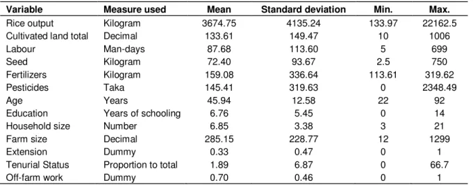
Table 1. Descriptive statistics of the variables for frontier and Tobit model.
Variable Measure used Mean Standard deviation Min. Max.
Rice output Kilogram 3674.75 4135.24 133.97 22162.5
Cultivated land total Decimal 133.61 149.47 10 1006
Labour Man-days 87.68 113.60 5 699
Seed Kilogram 72.40 93.67 2.5 750
Fertilizers Kilogram 159.08 336.64 113.61 319.62
Pesticides Taka 145.41 319.63 0 2348.49
Age Years 45.94 12.58 22 92
Education Years of schooling 6.76 5.45 0 14
Household size Number 6.85 3.38 3 21
Farm size Decimal 285.15 228.77 12 1299
Extension Dummy 0.33 0.47 0 1
Tenurial Status Proportion to total 1.89 6.87 0 66.7
Off-farm work Dummy 0.70 0.46 0 1
N, P and K stands for nitrogen, potash and phosphate; min and max denotes minimum and maximum.
Table 2. Tests of hypotheses results.
Null hypothesis LR statistics (χ2) Degrees of freedom p-value (Prob. > χ2) Decision
1. H0: αjk= 0 for all jk 83.61 21 0.00 Reject H0
2. H0: µ =γ =0 16.53 5 0.000 Reject H0
3. H0: α5= α51=… α55 =0 32.63 6 0.000 Reject H0
4. H0: η =0 4.24 1 0.000 Reject H0
variable ‘technical efficiency’ is a censored variable with an upper limit of one. The specification of the model is defined as (5):
i i it it
X
u
TE
=
β
+
(5) WhereTE
it*=
β
′
X
it+
ε
i and * t itTE
TE
=
if TE*>0,andTE=0Where
ε
i =N(0,σ
2),TE
it is the estimated technical efficiencyof the rice farmer;
X
iis the explanatory variables and β are unknown parameters. The explanatory variables are age (G is the age of the farmer in years); education (ED is the educational level of the farmer in schooling years); household size (HhS is the number of people in household including household head and permanent hired labour); farm size (in decimal); extension (with Ext a contact dummy with the value 1 is if farmer has contact with agricultural extension workers and the value 0 otherwise); tenure status (TU is proportion of rented-in land cultivated by the farm household); off-farm work (Off is a dummy value with 1 if farmer has chance to engage off farm work and the value 0 otherwise). ε is an error term which follows Gaussian process. We estimate the Tobit model with the help of STATA software package. Summary statistics of the variables used in all the models are presented in Table 1. Rice output includes all seasons and all rice varieties.Hypothesis tests
A set of hypothesis tests were performed by using likelihood-ratio (LR) statistic to determine the preferred functional form and the distribution of the random variables which is associated with the existence of technical inefficiency and the residual error term. Hypotheses test results are presented in Table 2.
First hypothesis was conducted to determine the functional form - Cobb–Douglas versus translog function. The null hypothesis of Cobb–Douglas production function is an adequate representation
)
0
:
(
H
oα
jk=
for all jk is strongly rejected, therefore the choice of translog production function seems a better representation of the production technology of rice farmers in Bangladesh.The parameter γ is the ratio of the error variances which is
γ
=
σ
u2/(
σ
v2+
σ
u2)
. The value of γ is in the range of zero (means no technical inefficiency) to one (means no random noise). The test of significance of the inefficiencies in the model rejected the null hypothesis (H
O:
µ
=
γ
=
0
)
and supports the existence of inefficiency effect.The null hypothesis of no technical change over time
)
0
:
(
H
Oα
5=
α
51=
α
55=
also got strongly rejected whichindicate that there is a technical change. The magnitude and direction will be determined and discussed in the next section.
At the end, the null of time varying technical inefficiency
)
0
:
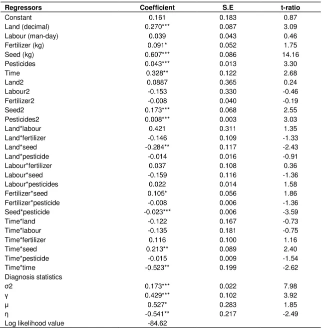
Table 3. Estimates ofstochastic production frontier using translog specification.
Regressors Coefficient S.E t-ratio
Constant 0.161 0.183 0.87 Land (decimal) 0.270*** 0.087 3.09 Labour (man-day) 0.039 0.043 0.46 Fertilizer (kg) 0.091* 0.052 1.75 Seed (kg) 0.607*** 0.086 14.16 Pesticides 0.043*** 0.013 3.30 Time 0.328** 0.122 2.68 Land2 0.0887 0.365 0.24 Labour2 -0.153 0.330 -0.46 Fertilizer2 -0.008 0.040 -0.19 Seed2 0.173*** 0.068 2.55 Pesticides2 0.008*** 0.003 3.03 Land*labour 0.421 0.311 1.35 Land*fertilizer -0.146 0.109 -1.33 Land*seed -0.284** 0.117 -2.43 Land*pesticide -0.014 0.016 -0.91 Labour*fertilizer 0.037 0.108 0.36 Labour*seed -0.159 0.116 -1.36 Labour*pesticides 0.022 0.014 1.58 Fertilizer*seed 0.105* 0.056 1.86 Fertilizer*pesticide -0.008 0.006 -1.36 Seed*pesticide -0.023*** 0.006 -3.59 Time*land -0.122 0.167 -0.73 Time*labour -0.135 0.181 -0.75 Time*fertilizer 0.116 0.100 1.16 Time*seed 0.213** 0.089 2.40 Time*pesticide -0.015 0.009 -1.54 Time*time -0.523** 0.199 -2.62 Diagnosis statistics σ2 0.173*** 0.022 7.98 γ 0.429*** 0.102 3.92 µ 0.527* 0.283 1.85 η -0.541** 0.217 -2.49
Log likelihood value -84.62
*, **, *** denotes significant at 10, 5 and 1% level respectively, the total number of observation is 219.
efficiency levels vary significantly over time as will be found out and discussed later.
RESULTS AND DISCUSSION Estimates of production function
The parameter estimates of the translog stochastic frontier production function are reported in Table 3. In our model, the estimated coefficients are directly the output elasticities because we have used the mean-differenced variables (xi =xi−x
*
).
The estimated coefficients on the land, fertilizer, seed and pesticides are significantly different from zero and have the expected positive signs. This indicates that all inputs tested (seed, fertilizer, land and pesticide) appear to be a major determinant of rice production in Bangladesh except labour. However, output elasticity of seed is the highest and estimated at 0.60 followed by land at 0.27 and fertilizer at 0.09, pesticide and labour at 0.04, respectively. Output elasticity of seed is estimated at 0.60 indicating that a 10% increase in seed use will increase output by 6%. Similarly, output elasticity of fer-tilizer is estimated at 0.09 indicating that a 10% increase in fertilizer consumption will increase output by 0.9%.
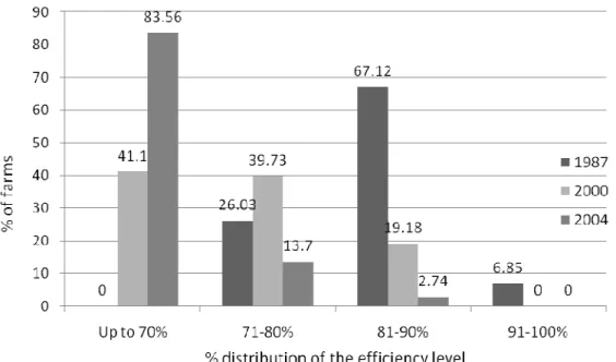
Figure 1. Distribution of the farms’ technical efficiency.
Table 4. Descriptive statistics of farms` technical efficiency (%).
Variables 1987 2000 2004
Mean efficiency 0.83 0.74 0.60
Standard deviation 0.05 0.07 0.10
Max 0.93 0.88 0.81
Min 0.72 0.58 0.39
The sum of elasticities is equal to 1.05 implying nearly constant returns to scale in production. The null hypo-thesis of constant returns to scale cannot be rejected. The coefficient on the time-trend variable is 0.33 and is statistically significant, which indicates positive techno-logical change over the studied period. In this case, the frontier has shifted towards the right. However, the coefficient of η (the time-varying efficiency effect) is negative (-0.54) and significantly different from zero. It indicates that the technical efficiency has declined over time (Table 3). Similar results were also found by Coelli et al. (2003). They found that technical efficiency declined over the time at the rate of 0.47% per annum. The result reveals that the farmers are very far from their frontier and the gap is increasing over the time, thereby implying that the production potential has not been realized at the farm-level. Figure 1 presents the frequency distribution of farm efficiencies over time. In 2004, 83.56% farms were in 0 to 70% efficiency group while in 1987 no farm was found in this low performance group. In 1987 highest percentage (67.12%) of farm belongs to 81 to 90% efficiency group, while in 2004, only 2.74% of farms were in this group.
The summary statistics of mean efficiency level are presented in Table 4. In 1987 mean efficiency level was 83%, in 2000 it stands at 74% and in 2004 it reduced to 60%. The estimates of 1987 and 2000 are slightly lower than those reported by Rahman (2007), Wadud and White (2000), Sharif and Dar (1996). It is evident from Table 4 that the mean efficiency level has declined substantially over time and has declined at an increasing rate. The variability of efficiency has also increased at an increasing rate over time.
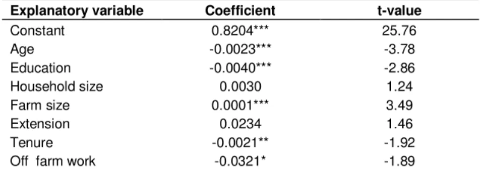
Efficiency elasticities
The results of efficiency elasticities are presented in Table 5. To calculate efficiency elasticities at first we find out the variables those effecting efficiency, then we calculate the efficiency elasticities of those variables. The regression results show that age, educational level, farm size, tenure status and opportunity of off-farm work have a significant impact on technical efficiency of rice farmers.
The elasticity estimate reveals that a 1% increase in age reduces technical efficiency by 0.002% (Table 5).
Table 5. Efficiency elasticities.
Explanatory variable Coefficient t-value
Constant 0.8204*** 25.76 Age -0.0023*** -3.78 Education -0.0040*** -2.86 Household size 0.0030 1.24 Farm size 0.0001*** 3.49 Extension 0.0234 1.46 Tenure -0.0021** -1.92
Off farm work -0.0321* -1.89
*, **, *** means significant at 10, 5 and 1% level respectively.
The negative sign of age implies that older farmers are technically less efficient than younger farmers. The result is expected as older farmers are likely to be more conservative towards new technologies, ideas and new practices than younger farmers. The similar negative sign of age were reported by Wadud and White (2000) and Balcombe et al. (2008).
The elasticity estimate reveals that a 10% increase in educational level reduces technical efficiency by 0.04%. An unexpected negative sign of education variable is not shocking, as the educational level of the people engaged in agricultural farming in Bangladesh is very low. In Bangladesh it is unlikely that educated people remain in agriculture because it seems to be less remunerative for them. Therefore, the negative influence of education on technical efficiency is not surprising at all. Similar results were also reported by Wadud and White (2000), Coelli et al. (2003), and Rahman and Shankar (2009).
The elasticity estimate reveals that a 10% increase in farm size will increase efficiency by 0.001% which is substantial. Farm size variable has the expected sign and is significant. Kamruzzaman et al. (2007) found similar results for Bangladeshi wheat farmers. The farm size positively influences technical efficiency implying that larger farms are more efficient than smaller farms. It is not unlikely that large farms can quickly utilize existing resources and might have a greater ability to access modern inputs on time.
Tenancy (defined as the proportion of rented-in land cultivated by the farm households) has a significantly negative impact on technical efficiency. It means that farms with a large proportion of rented-in land are less efficient than farmers cultivating owned land. The elasticity of tenancy estimate reveals that a 10% increase in the proportion of rented-in land to total cultivated land will decrease efficiency by 0.02%. The results is not unexpected because Coelli et al. (2002) and Rahman and Rahman (2009) also found similar results.
0ff-farm work also has negative impact on efficiency and it is significant. The elasticity of off farm work that is access to non-agricultural income) estimate reveals that
a 10% increase in the opportunity of off farm work will decrease efficiency by 0.3%. If the farmer has an opportunity to be engaged in off farm work then it is natural that they pay less attention to farming. Thus, opportunities for off farm work reduces technical efficiency, as expected. Rahman and Rahman (2009) and Balcombe et al. (2008) also reported parallel results.
However, household size (number of family members) and extension contact variables are not significant but have the expected signs. The extension contact help farmers to develop their analytical skills, critical thinking and creativity, and enable them learn to make better decisions. The poor effect of agricultural extension programs in farming is not unexpected. Similar results have been reported in past analyses of the productivity of agriculture in developing countries by Feder et al. (2004). The implication of positive sign of household size is that the larger households can substitute family farm workers with hired farm workers and, therefore, affect positively to technical efficiency.
Conclusions
The paper used the stochastic frontier production function with time varying farm effects model to examine the changes in technical efficiency at the farm-level for rice farms in Bangladesh using a balanced panel data for a cohort of 73 farms over a 17 year period (1987 to 2004). Our results indicate that the technological progress increased and has contributed to output significantly but that technical efficiency has declined over the study period. It was 60% in 2004 whereas it was 74 and 83% in 2000 and 1987 respectively. These numbers indicate that rice farmers are not fully efficient in Bangladesh and that the level of technical efficiency is decreasing over time at the farm-level. Thus, there remains considerable scope to increase production by improving efficiency of Bangladeshi rice farmers.
The farm-specific variables are used to explain technical inefficiencies and indicate that those farmers
who are young and have larger farms and do less off-farm work tend to be more efficient. Owner operators are clearly more efficient than the tenants. Extension services have a positive but not significant influence in increasing efficiency in rice farming showing their poor performance. Since the technical efficiency has declined over time, it is of utmost importance to design appropriate policies to improve efficiency at the farm level. From policy point of view, consolidation of land ownership can improve the technical efficiency level of rice farms. However, consoli-dation is a long term process. In short time inefficiency in rice farming can be reduced significantly by strengthening extension services and to increase their performance. We therefore, recommend paying more attention on this aspect in attempt to increase efficiency and to contribute to increased factor productivity and output growth.
REFERENCES
Aigner D, Lovell CAK, Schmidt P (1977). Formulation and estimation of stochastic frontier production models. J. Econom., 6: 21-37.
Amara N, Triode N, Labdry R, Romain R (1999). Technical efficiency and farmers’ attitudes toward technological innovations: the case of the potato farmers in Quebec. Can. J. Agric. Econ., 47: 31-43. Baffes J, Gautam M (2001). Assessing the sustainability of rice
production growth in Bangladesh. Food Pol., 26: 515-542.
Balcombe K, Fraser I, Latruffe L, Rahman M, Smith L (2008). An application of the DEA double bootstrap to examine sources of efficiency in Bangladesh rice farming. Appl. Econ., 40: 1919-1925. Baltagi BH (2005). Econometric analysis of panel data, 3rd edition,
Wiley, Chichester
Baltagi BH, Song SH (2006). Unbalanced panel data: A survey, Statistical Papers. 47: 493-523.
Battese GE, Coelli TJ (1992). Frontier Production Function, Technical Efficiency and Panel Data: with Application to Paddy Farmers in India. J. Prod. Anal.,3 (1):153-169.
BBS (2009). Statistical Yearbook in Bangladesh. Bangladesh Bureau of Statistics, Statistics Division, Ministry of Planning, Government of the People’s Republic of Bangladesh, Dhaka, Bangladesh.
Bravo-Ureta BE, Evenson RE (1994). Efficiency in agricultural production: the case of peasant farmers in eastern Paraguay. Agric. Econ., 10: 27-37.
Bravo-Ureta BE, Pinheiro AE (1993). Efficiency analysis of developing country agriculture: a review of the frontier function literature. Agric. Res. Econ. Rev., 22 (1): 88-101.
Coelli TJ (1994). FRONTIER Version 4.1: A Computer Program for Stochastic Frontier Production and Cost Function Estimation. Department of Econometrics, University of New England, NSW. Coelli TJ, Rahman S, Thirtle C (2002). Technical, allocative, cost and
scale efficiencies in Bangladesh rice cultivation: a non-parametric approach. J. Agric. Econ., 33 (3): 605-624.
Coelli TJ, Rahman S, Thirtle C (2003). A stochastic frontier approach to total factor productivity measurement in Bangladesh crop agriculture 1961-92. J. Int. Dev., 15: 321-333.
David CC, Otsuka K (1994). Modern Rice Technology and Income Distribution in Asia. Lynne Reiner Publishers, Boulder, Colorado.
FAO (2009). Bridging the rice-yield gap in the Asia-Pacific Region. RAP Publication 2009/16. Bangkok, Thailand.
Hayami Y, Ruttan W (1985). Agricultural development: an international perspective. Johns Hopkins University Press, Baltimore, MD. Hossain M, David L, Manik LB, Chowdhury A (2006). Rice Research,
Technological Progress and Poverty. PP. 56-102 in Michelle Adato and Ruth Meinzen-Dick (eds) Agricultural Research, Livelihoods and Poverty: Studies of Economic and Social Impact in Six Countries. Baltimore: the Johns Hopkins University Press.
Hossain M, Quasem MA, Jabbar MA, Akash MM (1994). Production environments, modern variety adoption, and income distribution in rural Bangladesh. In: David CC, Otsuka K (Eds.). Modern Rice Technology and Income Distribution in Asia. Lynne Reiner Publishers, Boulder, Colorado.
Hsiao C (2003). Analysis of panel data, 2nd edition, Econometric society monographs, 34. Cambridge University Press, Cambridge. Kamruzzaman MM, Manos M, Begum AA (2007). Evaluation of
economic efficiency of wheat farms in a region of Bangladesh under the input orientation model. J. Asia Pac. Econ.,11(1): 123-142. Kenny G (2001). Nutrient impact assessment of rice in major rice
consuming countries. FAO-ESNA Consultancy Report.
Kuznets S (1966). Modern economic growth: rate, structure, and spread. Yale University Press, New Haven.
Meeusen W, Broeck JVD (1977). Efficiency estimation from Cobb-Douglas production functions with composite error. Int. Econ. Rev., 18: 435-444.
Rahman HZ, Hossain M (1995). Rethinking Rural Poverty: Bangladesh as a Case Study. New Delhi, London: Sage Publication.
Rahman S, Rahman M (2009). Impact of land fragmentation and resource ownership on productivity and efficiency: The case of rice producers in Bangladesh. L. Use Pol., 26: 95-103.
Rahman S, Shankar B (2009). Profits, supply and HYV adoption in Bangladesh. J. Asia Pac. Econ.,14(1): 73-89.
Rahman S (2007). Regional productivity and convergence in Bangladesh agriculture. J. Dev. Areas, 41(1): 221-236.
Ruggiero J (2007). A comparison of DEA and the stochastic frontier model using panel data. Int. Tran. Oper. Res., 14: 259–266.
Salim R, Hossain A (2006). Market deregulation, trade liberalization and productive efficiency in Bangladesh agriculture: an empirical analysis. Appl. Econ., 38(21): 2567-2580.
Sharif NR, Dar AA (1996). An empirical study of the pattern and sources of technical inefficiency in traditional and HYV rice cultivation in Bangladesh. J. Dev. Stud., 32 (2): 612-629.
Sickles R (2005). Panel estimators and the identification of firm-specific efficiency levels in parametric, semi parametric and nonparametric settings. J. Econ., 126: 305-334.
Squires D, Tabor S (1991). Technical efficiency and future production gains in Indonesia agriculture. Dev. Econ., 29: 258-270.
Thiam A, Bravo-Ureta BE, Rivas T (2001) Technical efficiency in developing country agriculture: a meta-analysis. Agric. Econ., 25: 235-243.
Wadud M, White B (2000). Farm household efficiency in Bangladesh: a comparison of stochastic frontier and DEA methods. Appl. Econ., 32: 1665-1673.
Wilson P, Hadley D, Asby C (2001). The influence of management characteristics on the technical efficiency of wheat farmers in eastern England. Agric. Econ., 24: 329-338.