Cite this article as: Farkas, A., Porumb, B. (2020) "A Multi-Attribute Sales Comparison Method for Real Estate Valuation", Periodica Polytechnica Social and Management Sciences, 28(1), pp. 1–11. https://doi.org/10.3311/PPso.13897
A Multi-Attribute Sales Comparison Method for Real Estate
Valuation
András Farkas1*, Bogdan Porumb2
1 Institute of Entrepreneurship Development, Óbuda University, 1084 Budapest, Tavaszmező u. 15-17, Hungary 2 Bank of New York Mellon, Canada Square 1, Canary Wharf, E14 5AL London, United Kingdom
* Corresponding author, e-mail: [email protected]
Received: 17 February 2019, Accepted: 19 May 2019, Published online: 12 December 2019
Abstract
The theory and practice of real-estate valuation has attracted immense interest over the past decades. This paper is concerned with the sales comparison approach. First, a brief survey of some procedures used worldwide, the sales comparison by adjustments, the hedonic regression and the hedonic price index method, is presented. To improve the versatility of property appraisals a new valuation method, as a combination of multi-objective optimization (MOO) and multi-criteria decision analysis (MCDA) is developed. A unique feature of this model is that it enables the appraiser to evaluate the characteristics of a property on those scales of measurement to which they belong de facto. To comply with this objective, distinct metric distance functions on each scale of measurement, including the two qualitative scales (nominal and ordinal), are employed. After that, the physical worth of a property is derived as a weighted sum of the composite scores. This can be measured on an interval scale. To predict the monetary worth of a property, a simple linear regression model is developed. The benefits of the use of this multi-attribute valuation method is also discussed. A comprehensive real-world study showing the application of the procedure is included.
Keywords
real-estate valuation, sales comparison method, multi-attribute utility model
1 Introduction
The need for predicting real-estate prices by appropri-ate statistical tools emerged long ago to confirm buying, selling or construction decisions, property investments, real-estate funds, mortgage loans, project developments, insurance policies and taxation. The fundamental idea behind this major concept is the assumption that the het-erogeneous facilities (buildings, apartments, etc.) can accurately be described by their constituting components. Accordingly, in property valuation practice, real-estate is regarded as a bundle of its different characteristics (Brueggeman and Fisher, 2001). The actual number of these characteristics, also termed attributes, is very large, therefore, perfect information cannot be reached in real-world appraisals. Yet a rational choice on the relevant attributes for a given real-estate valuation model enables the appraiser to provide an unbiased estimate of the true, or at least a sufficiently fair market value of a particu-lar property. Supply and demand of transactions of prop-erties implicitly determine the characteristics' marginal contributions to their actual market prices.
This study focuses on the valuation of residential properties, i.e. single-family houses, condominiums and multi-family real-estates such as apartment houses. The scope of a systematic appraisal process should com-prise the following steps: the physical and legal identifi-cation of the property; the recognition of property rights to be valued; the collection and analysis of the gathered data for the characteristics of the property and, finally, the application of a convenient valuation technique (Brueggeman and Fisher, 2001).
There are three major widely recognized approaches used for real-estate valuation problems: sales comparison, income capitalization and costing approach. Each has specific objec-tives. This paper is concerned with the most widely used sales comparison approach which utilizes the transaction prices of highly comparable and recently sold properties in order to estimate the market value of the subject property, i.e. what a house or an apartment is really worth. The eco-nomic rationale of this concept is that no informed buyer/ investor would be willing to pay more money for a property
then the others who have recently paid for comparable prop-erties under the assumption that the general market condi-tions have not changed (Schulz, 2003).
The main contribution of this paper is the development of a new procedure for real-estate valuation called the Multi-Attribute Value Appraisal (MAVA) method. This technique appears to be capable of eliminating some inherent short-comings observable in the most frequently used contempo-rary approaches. We have attempted to write this paper to balance theory and application. An additional purpose of this paper is to provide practitioners with a sound concep-tual understanding of the sales comparison approach in the world of real-estate trading. Retaining the necessary aca-demic rigor, the focus is on the quantitative part of the appli-cations of the valuation model developed explaining how it works and showing how it can be applied/interpreted in the real-world real-estate business. The computer assisted solu-tion enables buyers and sellers to implement the method-ological advances successfully in order to arrive at a basis of a mutually favorable agreement for both parties on the ultimate transaction price of the property under bargaining.
While desiring to stress that statistics should be used in the everyday private affairs of property appraisals, the authors realized that it is difficult to directly employ such an approach in today’s practice. Therefore, a compre-hensive case study will be used primarily from the up-to-date real-estate business, where readers can easily follow the steps and the content described in a precise manner. Although including certain unavoidable risks, the attached instructions and guidance aid the appraiser in construct-ing a solid report in each particular case with an efficient method of collecting and analyzing the pertinent informa-tion in a coordinated framework toward the goal of obtain-ing reliable results. In addition, we have strived to keep our property valuation model both controllable and repeatable.
Nowadays, mobile apps are widely available in this field, utilizing artificial intelligence and big data environment including the integration of GIS (geographic information system) for a complete visualization of the mass appraisal process. This has become a competitor of the conventional valuation space via digitization of the evaluation process. These appraisal apps, with fully customizable templates, make the procedures more simple and efficient to fit user's individual needs and, thus, providing special appraisal services. They are able to create an easy manner to obtain a price estimate of a house or an apartment for a client in an electronic and streamlined way. With these tools
a report can be generated and forwarded to the individual or company that requested the appraisal. The most popular free home value sites on the net are, e.g. Zillow, Trulia and Realtor, which can be accessed from iPhones, or tablets. We believe that our methodology would be used in these apps and, thus, expand the scope and usefulness of them.
The paper is organized as follows. In Section 2, we pres-ent a brief overview of the existing sales comparison approaches for real-estate valuation. The formal descrip-tion of MAVA is discussed in detail in Subsecdescrip-tion 3.1. In Subsection 3.2, a real-world application is shown includ-ing the necessary numerical computations and the evalua-tion of the findings.
2 A brief survey of sales comparison approaches
In this section we present a brief description of three meth-ods used extensively in this field of interest.
2.1 Sales comparison by adjustments
As a result of the first three steps carried out in a valuation process the required information (data) for a given set of comparable properties, Ω :={ ωj }, j =1, …, J, and for the set of the relevant characteristics (attributes), Λ :={ λk },
k = 1, .., K, are available for the valuer. Next, the trans-action prices for differences in characteristics related to the subject property have to be adjusted (Schulz, 2003). For this purpose the appraiser needs to know the proper adjustment factors. Since there are no unified techniques to derive these corrective measures, they are assessed by the appraiser, based on his/her talent and/or intuition. Sometimes he/she guesses them in percentages. The rela-tive importance of each attribute should also be taken into consideration by using weighting factors in the procedure.
Isakson (2002) developed a linear algebraic model to formally describe this approach. There it is assumed that all transactions occurred in the preceding period, t−1, and the transaction price of a comparable property (P) is a lin-ear function of the characteristics. Then, for period t, what he called the individual values, vj t,
S , for the subject
prop-erty (S) are computed by the following matrix equation as the entries of vector (Isakson, 2002):
vt pt ext Xt a t S P S P T = −1+
(
− −1)
= …1 T , , , , (1)where, for period t−1, pt−1
P denotes the vector of the
trans-action prices, pj t,−1 P ,
j = 1, …, J, of the comparable proper-ties sold with the vector of the characteristics xt−1
P , entries
of which are xj k t, ,−1 P ,
are usually measured in appropriate units like price per square meter. The matrix Xt−1
P stands for the respective
characteristics with the elements, xj k t, ,−1 P ,
j = 1, …, J, and
k = 1, …, K. The characteristics' data of the subject prop-erty are entered in vector xtST
. A column vector e is also introduced whose elements are all equal to one. The col-umn vector of the adjustment factors is denoted by a, entries of which are ak , k = 1, …, K. Next, the appraiser has to weight the individual values of vector vtS by using
the positive weights, wj t,
S , where these weights sum to one.
A difficult problem with this method is the deriva-tion of the adjustment factors. The appraiser has to rate many unknowns including the magnitudes of these cor-rective measures, therefore, the performance of the valu-ation process may be affected by subjective guesses and judgments made by the appraiser. Also, it may occur that the observed properties are not completely comparable.
2.2 Sales comparison using hedonic regression
Considering that the real-estate valuation problem bears a statistical nature, a well-known multivariate tech-nique, the multiple regression analysis is apparently be used for estimating the value-determining characteris-tics, and, ultimately, the transaction price of the subject property. By employing this statistical tool, the transac-tion price of a property in a given time interval is a func-tion of an aggregate price level, the property's character-istics and an unexplained part, assumed to be random. This method, called hedonic regression, is able to derive the marginal contributions of the characteristics of the comparable properties and was first introduced in this area of interest by Bailey et al. (1963). The economic pur-pose of the hedonic regression aims to obtain estimates of the willingness to pay for, or marginal cost of producing, the different characteristics (Schulz, 2003).
Making use of the above considerations and the nota-tions as those of in Subsection 2.1, we can write that (de Haan and Diewert, 2013):
ptS f xPj t xj t j t j K P P J =
(
, ,1 −1,…, , ,−1,ε ,−1)
, = …1, , , (2) where t = 1, …, T+1, and εj t,−1P is a random error term,
assuming that Exp εP
j.
( )
=0, and Var εPj.
( )
=σ2 which isconstant for all j in each time period. To estimate the mar-ginal contributions of the characteristics by employing multiple regression, Eq. (2) must be specified as a para-metric model. The basic and simplest forms of the two best known hedonic regression equations are the linear hedonic model (de Haan and Diewert, 2013):
ptS=β0,P 1+
∑
βPk t−xj k tP − +εPj t− j= … J 1 t j k − = , , 1 , , 1 , 1, 1, , , (3)and the logarithmic-linear hedonic model (recognized that the transaction price distributions can often be skewed) (de Haan and Diewert, 2013):
lnpt , ,k t xj k t, , j t, , j , , , S P P P K P J =β0, 1+
∑
β − − +ε − = … 1 t j k − = 1 1 1 1 (4) where β0 P is theY-intercept and the βkP's stand for the
characteristics' parameters to be estimated from appropri-ate samples by applying the ordinary least-squares (OLS) method. These coefficients indicate the marginal changes of the price with respect to a change in the k-th character-istic of the property. For obtaining more efficient estimates and improving the model validation phase the characteris-tics may be transformations, or more complex functional forms, or interaction of continuous variables, since the inde-pendent variables can enter the linear model in a nonlinear fashion as well. In the real-estate practice, many explanatory variables are categorical rather than continuous and repre-sented by a set of dummy variables (either 0 or 1). In these cases the regression problem is referred to a dummy variable hedonic model (de Haan and Diewert, 2013).
A great advantage of the hedonic regression approach is that it can handle large data sets, see e.g. some U.S. real-estate data sets in Woodard and Leone (2008) or in De Cock (2011). Furthermore, this approach is suitable for mass apprais-als including automated valuation, see this problem e.g. in (Shiller and Weiss, 1999). Once the regression "hyperplane" has been fitted, the expected price for a given property can be computed via suitable computer packages.
In the real-estate practice, the majority of the rele-vant characteristics are very hard to quantify and are not systematically recorded in data sets. An appraiser vis-iting the subject property would take such "soft" factors into consideration. Sometimes they fail and consequently there are missing data (Schulz, 2003). Hence, the perfor-mance of the model may become significantly distorted. Another problem often arises in hedonic regression, namely when the model suffers from severe multicollinear-ity, and thus, the parameter estimation will become seri-ously biased. Similarly, in many applications, the violation of some other assumptions underlying the use of the model cannot be eliminated, such as e.g. the issue of heteroskedas-ticity. Nevertheless, by taking the logarithm of the prices the harmful effects of non-equal variances can be released.
Furthermore, caution must be exercised when using average prices, because they may be misleading, since they are biased estimators of the common price components
as it was shown by Case and Quigley (1991). The number of the characteristics as regression parameters, βkP's that
can be entered a hedonic regression model is rather lim-ited as compared to those which would be necessary to involve in the applications. Finally, in the authors' practice, we have often experienced that many real-estate agencies are usually being rather reluctant to use these sophisti-cated statistical methods for property valuation purposes.
2.3 Sales comparison using hedonic price indexes
Another approach that is frequently applied in real-estate valuation attempts to compile an indicator termed a hedonic price index (Brachinger and Diewert, 2002). The basic idea behind any of such indexes is to compare the hedonic price of a particular property at two different points in time hold-ing the status of the property constant. There are two major procedures: the characteristics prices and the imputations approach. They generate different statistical indexes like the Laspeyres, Fisher and Paasche indexes.
Hedonic pricing has some drawbacks, among others a limited sensitivity to the environmental differences. Also, they are not capable of incorporating external fac-tors of regulations, such as taxes and interest rates which have significant impact on prices. The interested reader may find detailed information about these indexes in the excellent work of de Haan and Diewert (2013) including their use for property valuation.
3 The multi-attribute value appraisal (MAVA) method
In this section we show the development of a combined multi-objective optimization (MOO) and multi-crite-ria decision analysis (MCDA) technique, called Multi-Attribute Value Appraisal (MAVA) method that may be applied for any real-estate valuation based on sales com-parison. The conventional valuation approaches attempt to provide an estimate of the market value of a particu-lar property in a relatively short time period. The mar-ket value refers to the prospective price of a building or a house or an apartment. According to the US standards (Brueggeman and Fisher, 2001), the transaction price is defined as the most probable price, while in the German regulations it is declared as the expected price of the prop-erty under study (Schulz, 2003). Both definitions assume that the price is not affected by undue stimulus committed by the seller and/or by the buyer.
MAVA applies just a different strategy. It distinguishes between the value of a property and the transaction price of it. The monetary worth of a property is expressed as
the amount of money it was sold for in the market in the preceding time period, while the physical worth of a prop-erty is regarded a measure of the benefit or utility pro-vided by a house or an apartment. The method first deter-mines the physical worth of a property by a computed
value index, then it establishes a statistical relationship in order to estimate the monetary worth of a property which is intended for sale or purchase. The latter notion is mani-fested in the expected selling price.
The seminal models of multi-attribute utility theory postulate that the preference of an individual towards a choice object is related to its distance from his/her ideal object which may well be a hypothetical object, see e.g. Dyer and Sarin (1979); Horsky and Rao (1984); Hwang et al. (1993) and Zeleny (1974). The closer the object is to the ideal one, the greater the preference for it. The distance is a compound measure which takes into account the loca-tion of each alternative (properties) on several attributes (set of criteria) which characterize them.
A variety of these methods are used in practice but the majority of them have been designed to evaluate the alternatives on one particular scale of measurement only. Contrary to this manner, the attributes have to be assigned to different types of scales, since the alternatives of an ill-structured decision problem are usually charac-terized by a great number of attributes which may have entirely diverse features. A given scale is homogeneous and thus, only those transformations are allowed which let the inherent structure of that scale to be invariant.
MAVA was constructed to be capable of handling both tangible and intangible attributes simultaneously. Our approach requires that non-quantifiable and quantifi-able attributes be treated in a different manner. Therefore, the matrix of the input data is partitioned into four block matrices (nominal, ordinal, interval and ratio). Every attri-bute is then assigned to that block which represents its associated scale of measurement. Hence, the elements of this matrix are mixed, i.e. they appear in the forms of binary variables, rank numbers and numerical quantities with their accompanied units of measurement. A weighting number is also computed and assigned to each attribute to express its relative importance with respect to the others.
At this point, the question can be raised as to whether there is any difference between the multivariate statistical method called multidimensional scaling (MDS) and MAVA. The answer is yes. MDS defines the visual distances of sim-ilarity between different objects on a 2D plane or a 3D space which can be interpreted in a pairwise manner. Since here,
the evaluation process can only be accomplished by dimen-sional reduction (the underlying problem is generally n -di-mensional), it involves loss of information and biases in the true distances. In contrast, MAVA is a multiple-criteria eval-uation and aggregation method using metric similarity func-tions, so that the attributes are assigned in advance to their original measurement scales. The final results are numerical (on an interval scale) and they do not appear on a graphical representation map as they do in MDS.
3.1 Formal description of the method MAVA
This method conforms to the theory of measurement (Stevens, 1951) concerning its basic concept such that each attribute contained by the set of the characteristics is first assigned to its corresponding scale of measurement. The properties have to be evaluated with respect to each attribute. After the evaluation process has been completed, the scores (ratings) which the properties have received from the appraiser are available in an input data table like the one displayed in Table 1, in Subsection 3.2. Following this, a hypothetical reference property is defined, which is arbi-trarily chosen by the appraiser. It either represents the tar-geted (desired) quality of a property with respect to each attribute, or it can be composed of the best values of each existing attribute. This hypothetical property may also be referred to as a benchmark, that is a standard, by which the evaluated properties are compared and measured.
Obviously, every owner wishes his/her house or apart-ment to be located to the benchmark as much as possi-ble. In other words, the apartment having the best physical worth is the one that is closest to the standard. MAVA mea-sures "closeness" in terms of distances, by defining appro-priate distance functions for each scale of measurement. The subjective judgments, guesses and the measurements will be transformed to computed differences between the single properties and the benchmark property. They are represented on an intervalscale by an aggregate compos-ite score called a value index of a property. Hence, MAVA is a scaling method of absolute measurement and may be used for competitive benchmarking as well.
We are given the matrix of the input data, where the data were assessed and/or collected by the appraiser(s). Let
A=
[ ]
aik , i=1 2, ,…, ,m k=1 2, ,…, ,n (5)denote the matrix representing n properties. The n col-umns give for every option the scores of the m variables (rows) representing various characteristics of these prop-erties. In matrix (Eq. (5)), a numerical value (also called
a score) is assigned to each entry, aik , which is either elicited from subjective experts' judgments or arisen from measurements. Thereby, the nature of a partic-ular data may be of a qualitative or a quantitative type. One single data represents a part-worth which contributes to the total physical worth of a property. Every column vector akof matrix A is partitioned, therefore it represents a composite vector, ak akN a a a
kO kI kR
= ( ), ( ), ( ), ( ), having four
block vectors. Thus, A includes variables of mixed type, where N refers to nominal (usually binary), O to ordinal,
I to interval and R to ratio variables. Of course, in a con-crete case, variables of any type may be missing.
A column vector b = [ bi ], i = 1, …, m, called a reference vector, is constructed and added to matrix A as its n+1-th column. Vector b represents the reference property, entries of which receive the "best" values of each attribute in the course of the evaluation process and it has the same ele-ment-wise structure as that of vector ak . Assigned numeri-cal values used in this model are: [0, 1] on a nominal snumeri-cale; [1, …, 10] on an ordinal scale; [0, …, 100] percentage or point on an interval scale and the actual numerical values, i.e. data from measurements on a ratio scale.
Because the ratio (and sometimes the interval) variables usually have different units of measurement, the row vec-tors, ai( )RT
(and ai( )IT
), are standardized so that we equate their means equal to zero and their standard deviations to one. For example, the standard deviations for the ratio variables can be computed in the following way:
s n a n a iR ikR i m ikR i m R R R R ( ) ( ) = ( ) = = − − ( ) ( ) ( ) ( )
∑
∑
1 1 1 2 1 1 2 , (6)where i =1(R), …, m(R); k =1, …, n. Using Eq. (6), the
stan-dardized elements can be obtained as
′ =( )
(
−)
( ) ( ) ( ) a s a a ikR iR ik R iR 1 . . (7)In the case of group decision making, a representative group of respondents (experts) is formed. Every mem-ber has to evaluate each alternative by supplying his/ her judgments on each qualitative variable on the nomi-nal and ordinomi-nal scale attributes. It is highly recommended that the number of voters l, l = 1, …, q, be at least: q = 5-6. In the case of more than one voter, to find the compromise ranking, we refer to the paper of Seiford and Cook (1982).
The general form of the real-estate valuation model used in MAVA is as follows:
Dkl w dil ikl k n l q i m kl = ⋅ + = … = … =
∑
1 1 1 ε , , , , , , , (8)where Dkl is the overall distance of property k from the
ref-erence property related to the l-th voter; wil is the weight
of attribute i; dikl is the distance of the k-th property
from the reference property on attribute i, which can take a number of forms: dikl f b a
i i ikl
=
(
−)
, where aikl denotesthe normalized scores on nominal, ordinal and interval scales (their sum equals one) and the standardized scores on ratio scale; εk is the value of an error random variable
which includes measurement errors and voters' uncertain-ties. Assumptions underlying the proper use of the valua-tion model (Eq. (8)) are: Exp
( )
εk =0, and Var( )
εk =σ2which is constant for all k.
To assess the weighting factors of the attributes, wil,
equal weighting methods or rank order weighting meth-ods (rank-order centroid weights or rank-sum weights), or the so called swing weight method are proposed; see these procedures e.g. in Jia et al. (1998). If the number of the attributes is small (not more than 6-7), the analytic hierarchy process (AHP) method can also be a good choice for this procedure (Saaty, 1977). The weights are then nor-malized so that they sum to unity.
The main objective is to obtain the value indexes, vkl, k=1,…,n, which are composed of the part-worths of the properties on the different scales of measurement. By aggregating them, the "total" (overall) physical worth of a property is determined. These measures are derived by the distance functions over the set of the compos-ite vectors. They represent the closeness (similarity) of the properties to the benchmark property and are com-puted as: vkl = −1 Dkl. In other words, this measure
indi-cates the "goodness" or utility of a property yielded on an interval scale that varies from 0 to 100 percentages or points. Clearly, the vector of the benchmark property has a value index of 100, since it represents the reference prop-erty. The "best" property, denoted by A*, yields for the l-th
voter (we note that in case of real-estate valuations, usu-ally, l = 1, because there is only one voter, the appraiser):
Al v k n l q
k k
l
∗ =max
{ }
, = …1, , , = …1, , . (9)In real-world appraisals, the set of attributes generally con-sists of a number of variables that can only be measured on nominal and/or on ordinal scales. In such cases, the respec-tive distances should conform to the theoretical requirements of metric distance functions. Otherwise, the corresponding block vectors cannot be transformed up to an interval scale. The mathematical assumptions that a metric distance func-tion must satisfy are as follows (Späth, 1985):
• Axiom 1 (Metric Requirements.) For any three com-posite vectors, x, y, z, the following relations must hold 1. d (x, y) ≥ 0,
2. d (x, y)=0, when x = y, 3. d (x, y) = d (y, x),
4. d (x, z) ≤ d (x, y) + d (y, z).
• Axiom 2 (Proportionality.) The distance between any two composite vectors is proportional to the degree of intensity.
In the rows of the data matrix A the distance measure,
di , usually takes on different functional forms:
1. The distance measure for the i-th attribute,
diN aijN aikN
( )
(
( ) ( ))
, , of any two nominal vectors,
j-th and k-th, denoting them simply as x y, ∈N, is the Tanimoto (also called Jaccard) coefficient (Sokal and Sneath, 1963):
di( )N
(
x y)
= − + + = + + + , 1 α , α β γ β γ α β γ (10) where α β α γ α =(
)
= − = − ∈∑
∑
∑
min , , , , . x y x y i N i i i i i i i2. The distance measure for the i-th attribute,
diO aijO aikO
( )
(
( ) ( ))
, , of any two ordinal vectors, j-th and k-th, denoting them simply as x y, ∈O, is the Soergel number (Soergel, 1967):
d x y x y x y x y x y i iO i i i i i i i i i i i i i i ( )
(
)
= + −(
)
+ −(
)
∑
∑
∑
∑
∑
∑
, min , min , , 2 ∈ ∈O. (11) 3. For any two interval and ratio vectors, j-th and k-th,denoting them either x y, ∈I, or x y, ∈R, and introducing the L2norm of a vector x, we have
x2 x x
2
=
∑
ixi = i I∈ i R∈T
, , or .
The distance measure of the i-th attribute,
di(I R, )
(
aij(I R, ),aik(I R, ))
, is the well-known Euclidean-metric: di I R, , . ( )(
x y)
= x y− =(
x y−)
(
x y−)
2 T (12)In Farkas (2004), the necessary proofs are given to show that the metric properties hold for Eqs. (10) and (11). MAVA applies the distance function of the compos-ite vectors, dC in an additive fashion, since the metric properties hold for its component distance functions and the scales are linear. Therefore, the composite vector is
also metric. Furthermore, it is unique and for each row, 0 ≤ di ( aik , bi ) ≤ 1, i = 1, …, m, holds. The proportionality unit is taken to be one.
Proposition.If the metric properties hold for the dis-tance functions of the nominal, ordinal, interval and ratio vectors of a data matrixA defined in Eq. (5), the composite distance vectordC is also metric. Furthermore, it is unique and measures the true distance between any two compos-ite vectors of A on an interval scale.
Proof. The proof readily follows from the consider-ations which have been made thus far. □
With the pairwise distances, between each composite vector and the reference vector b, a Pareto optimal solution for the value indexes, vkl = −1 D kkl, = …1, , ,n l= …1, ,q,
has been obtained. They specify the physical worth of the properties.
Once the value indexes of the properties have been deter-mined, the appraiser has to establish a possibly sound sta-tistical relationship between the value indexes as inde-pendent variables and the selling prices as deinde-pendent variables, i.e. between the physical and the monetary worths of the properties. Given the known transaction prices of the properties sold in the preceding period, t−1, a simple lin-ear regression model appears to be adequate to this problem. The authors' experience with this strategy was very favour-able and the steps are discussed concisely in what follows.
The value indexes are used to predict the selling prices of the properties. First, the point estimates, b0 and b1 , of the two parameters, β0 and β1 , of the population regres-sion model are produced using randomly chosen sample data from the population of properties. After the regres-sion equation has been fitted to the sample data points, it is especially important to check the assumptions underlying the proper use of this model. Although the examination, whether or not the assumptions of the regression model have been met is a complex task, yet the construction of residual plots is very helpful to carry out this analysis.
Next, at a stated level of significance, the statistical test of the usefulness of the model developed follows using com-mon inference making techniques. Finally, if the model is statistically significant, the fitted regression equation can be used for prediction and estimation purposes. Both the mean (expected) selling price given a particular value index, or the selling price of a "new" property which was not contained by the original data set, can be estimated. In this simple way, the appraiser can not only estimate the price of a prospective real-estate object, but he/she is able to provide reliable lower and upper limits on the prices by using the calculated confi-dence and prediction intervals.
3.2 A real-world application of the method MAVA
This study covers a number of 62 apartments/flats (pop-ulation) built in multi-family houses and sold in the first half of 2018. They are located in a hill-side area of the cap-ital city of Budapest, Hungary. A simple random sample of
n = 12 apartments, ΩΩ:=
{ }
Ak , k = 1, …, n, was taken from the population of properties and their selling prices, pk ,k = 1, …, n, were recorded. In order to assess the physical worth (value indexes), vk , of the apartments a three mem-ber expert group was formed from experienced appraisers. This group determined the common set of the characteris-tics, (attributes), ΛΛ :=
{ }
Ci , i = 1, …, m. This set of criteria will be used to evaluate each apartment with respect to every criterion. In this respect, a desirable goal is to have independent attributes, nevertheless, it is hard to cope with this assumption in practice.In the following stage of the study the weights of the attri-butes had to be derived. Since, in the case of property eval-uation, it cannot be assumed that the attributes are equally important the swing weight procedure appeared to be appro-priate. The group of appraisers was asked to set up the rank order of the attributes in terms of their associated value ranges. Assuming that each attribute is at its worst possible level, they were asked which attribute they would most pre-fer to change from its worst to its best level. The attribute chosen has the most important value range. This attribute is assigned a weight of 100. Next, proceeding this process similarly, the group rank ordered the attributes and assigned relative importance weights to every attribute according to their value ranges between 0 and 100. The last step was to normalize these weights to obtain the normalized swing weights, w1 , …, wm . They are presented in Table 1. The rank ordered m = 15 single attributes, with their rank numbers in descending order and the corresponding ratings attached to them (in brackets), are given below:
1. Location of the property (100) — classification of environmental and geographic area
2. Legal status (70) — legal and financial circum-stances of the property
3. Saleable floor area of apartment (70) — net floor area +1/2 balcony area +1/4 terrace area
4. General condition of apartment (65) — finish, built-in materials, covering, remodel date, etc.
5. Overall condition of building (60) — exterior and interior shape, style, remodel date, etc.
6. Number of rooms (55) — excluding bathroom(s) and kitchen
7. Type and quality of utilities available (52) — electricity, gas, water, air-conditioning, wifi
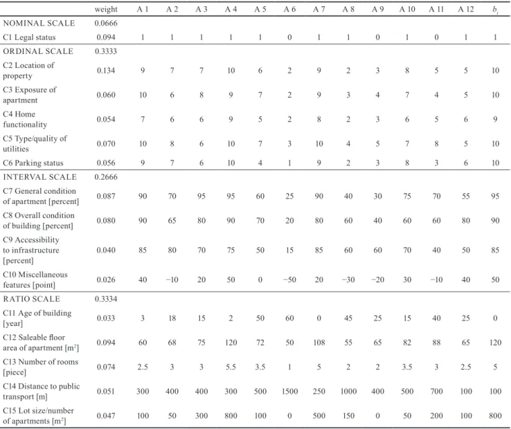
Table 1 Input data: attribute scores and the normalized aggregated and single attribute weights and the elements of vector b weight A 1 A 2 A 3 A 4 A 5 A 6 A 7 A 8 A 9 A 10 A 11 A 12 bi NOMINAL SCALE 0.0666 C1 Legal status 0.094 1 1 1 1 1 0 1 1 0 1 0 1 1 ORDINAL SCALE 0.3333 C2 Location of property 0.134 9 7 7 10 6 2 9 2 3 8 5 5 10 C3 Exposure of apartment 0.060 10 6 8 9 7 2 9 3 4 7 4 5 10 C4 Home functionality 0.054 7 6 6 9 5 2 8 2 3 6 5 6 9 C5 Type/quality of utilities 0.070 10 8 6 10 7 3 10 4 5 7 8 5 10 C6 Parking status 0.056 9 7 6 10 4 1 9 2 3 8 3 6 10 INTERVAL SCALE 0.2666 C7 General condition of apartment [percent] 0.087 90 70 95 95 60 25 90 40 30 75 70 55 95 C8 Overall condition of building [percent] 0.080 90 65 80 90 70 20 80 60 40 60 60 80 90 C9 Accessibility to infrastructure [percent] 0.040 85 80 70 75 50 15 85 60 60 70 40 50 85 C10 Miscellaneous features [point] 0.026 40 −10 20 50 0 −50 20 −30 −20 30 −10 40 50 RATIO SCALE 0.3334 C11 Age of building [year] 0.033 3 18 15 2 50 60 0 45 25 15 40 25 0 C12 Saleable floor area of apartment [m2] 0.094 60 68 75 120 72 50 108 55 65 82 88 65 120 C13 Number of rooms [piece] 0.074 2.5 3 3 5.5 3.5 1 5 2 2 3.5 3 2.5 5 C14 Distance to public transport [m] 0.051 300 400 400 300 500 1500 250 1000 400 500 700 100 100 C15 Lot size/number of apartments [m2] 0.047 100 50 300 800 100 0 500 150 0 50 200 100 800
8. Exposure of apartment (45) — geographic situa-tion, panorama, proximity to other houses, privacy
9. Parking status (42) — garage size, location, con-dition, driveway, or street parking conditions only
10. Home functionality (40) — habitability comfort, rentable opportunity, investment perspectives
11. Distance to public transport (38) — accessibil-ity for bus, metro, suburban train stations
12. Lot size/number of apartments (35) — area, shape, configuration of surrounding garden of the house
13. Accessibility to infrastructure (30) — shopping malls, schools, health centers
14. Age of building (25) — construction date
15. Miscellaneous features (20) — positive and/or negative aspects not covered in other categories, e.g. elevator
In the next phase of the study the attributes of the apart-ments were assigned to the appropriate scales of measure-ment. Then, one professional appraiser evaluated each of the 12 apartments on these scales, at each site. Both sub-jective judgments and physical measurements were per-formed. For the ordinal variables, a discrete 10-grade [1-10] scale was established and the rank numbers were verbally interpreted. These are in a descending order, in turn: supe-rior; excellent; very good; good; above average; average; below average; fair; poor; extremely poor. For the interval variables he used a [0-100] percentage (or point) scale to execute the evaluation of the apartments by providing ade-quate ratings as much as possible.
The scores resulted in the multi-attribute evaluation for the 12 apartments are shown in Table 1. Observe here that the attributes, Ci , i = 1, …, m, have been rearranged with respect to the scales they truly belong to, hence, they
were renumbered in this table. In Table 1, the attribute scores, the normalized aggregated and single weights for the different types of the scales of measurement and the ele-ments of the reference vector b (best values) are displayed.
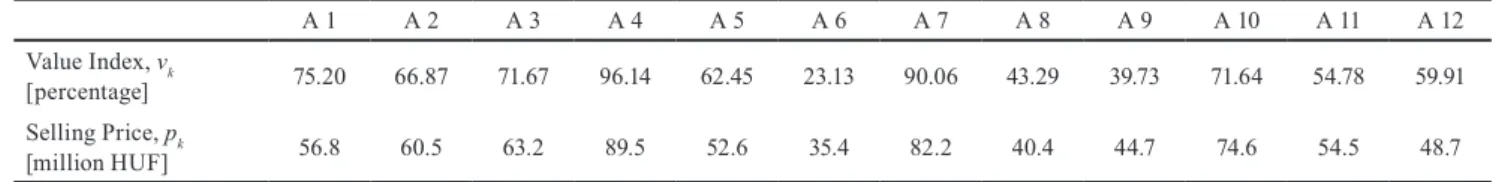
Now we turn to the computation of the value index of each property as a bundle of its different characteris-tics. A computer program was written in FORTRAN 95 language to compute these indexes. They are presented in Table 2 together with the associated selling prices of the comparable properties which were recorded previously. From Table 2,itcan be seen thatthe level of qualification of the "best" property, A*, is A4⇒96 14. percentage.
The starting point of the second stage of MAVA is to specify the nature of the relationship between the indepen-dent variable (the value index) and the depenindepen-dent variable (the selling price). The analysis of the scatter plot diagram, using the data given in Table 2, led us to the conclusion that a straight line can be drawn to fit reasonable well through the data points and the points scatter randomly about this line. It means that most of the variation in the selling price is accounted for by relating it to the value index, i.e. to the physical worth of the properties.
Now, we have to check whether or not the assumptions of the simple linear model have been met. The required computations were made by the package SPSS 20.0. The fitted regression equation with the estimated parame-ters, b0 and b1 , of β0 and β1 , yielded
yˆ=12 141 0 738. + . x. (13)
The sample coefficient of determination is: r2 = 0.859,
which means that the value index explains a considerably large proportion of the variability in the prices. (Adjusted
r2 = 0.845.) The sample coefficient of correlation is:
r = 0.927, showing that there is a strong positive linear relationship between the variables; the slope of the regres-sion line is significant: p = 0.001 at the level of α = 0.05. The Durbin-Watson statistic is: DW = 1.764 indicating that the error terms are uncorrelated enabling the model for inference making purposes. Normality of the error
terms also applies. However, there is a slight suggestion for nonconstant error variance of the residuals for larger values of the value indexes.
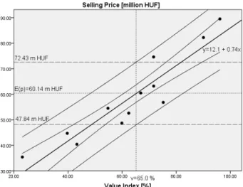
One of the major goals of the established model is to use it for prediction. Suppose now that a new seller arrives at this market and the appraiser wishes to know the expected sell-ing price for his/her property in this market. This new ssell-ingle observation past the present 12 apartments in our sample. Let its value index be exactly 65 percent, as it was deter-mined by the appraiser. At this setting, the predicted price yields: 60.14 million HUF, and the 90 % prediction inter-val is: [47.84 – 72.43] (see in Fig. 1). Hence, the appraiser can be 90 % confident that this next sale will lie between these limits. Observe that this interval is rather wide due to an additional variability inherent in the prediction problem as opposed to the mean estimation, where the confidence interval is much narrower: [56.71 – 63.56] belonging to its associated mean value of 60.14 million HUF.
In predicting a new single price observation pnew , we are confronted with the variability in estimating the mean, plus the additional variability of the specific distribution of P, given a specific value of vnew . Thus, in predicting a new single observation, we must take into consideration the variability in fixing the location of the distribution (mean estimation) and take into account the variability within this distribution (since we are attempting to predict a specific value that belongs to this distribution).
This problem is illustrated in Fig. 1, where the upper and lower limits are displayed for both estimation prob-lems. It can also be seen that in the original sample, there are four properties whose selling prices were either over-valued, i.e. they were sold very well, or underover-valued, i.e. they were sold rather poorly.
As readily seen in Fig. 1, one point lies above the upper confidence bound (it is a curve), whilst three points are below the lower confidence bound (it is a curve) drawn to the fitted regression line defined in Eq. (13). This fact also contributed to have rather wide prediction intervals for the particular value indexes, vk .
Table 2 The value indexes and the selling prices of the properties
A 1 A 2 A 3 A 4 A 5 A 6 A 7 A 8 A 9 A 10 A 11 A 12 Value Index, vk
[percentage] 75.20 66.87 71.67 96.14 62.45 23.13 90.06 43.29 39.73 71.64 54.78 59.91 Selling Price, pk
4 Conclusions
In this paper a new sales comparison method has been devel-oped for real-estate valuation. This method seems to outper-form several other approaches since it reveals a clear and easy to understand link between the physical and the mone-tary worths of a particular property in a given market.
This method performs well (all statistical assumptions are met), if the real-estate market is in balance, i.e. the sup-ply and the demand for the sales and purchases of the apart-ments are, at least in a relatively stable equilibrium.
Under the above circumstances evidence exists that MAVA is capable of eliminating the multicollinearity problem of hedonic regression. Besides, it reduces heteroskedasticity considerably. Therefore, MAVA produces statistically sig-nificant and reliable outcomes.
However, if the real-estate market is not in balance, then the effectiveness of the statistical model is worsening and the results may become more or less biased. Of course, there is room to further develop the method in the future. One useful direction would be the construction of non-lin-ear measurement scales for the attributes which attain a minimum or a maximum within a given interim range of their value indexes.
The authors' earlier observations reflected to a fre-quently occurring case in the real-estate market practice. Many buyers are eagerly seeking to find an apartment or a house with only one or two objectives (attributes) in mind as being extremely important for them. We stress that appraisers should know better the preferences of the buy-ers, otherwise, there may be a discrepancy between their exclusive claims and a "standard" weighting factor sys-tem. There is no unique such a system for any real-estate market, but a variety of adequate weighting systems has to set up by the appraisers in order to avoid misleading evaluations.
Fig. 1 Prediction and confidence bounds about the mean selling prices
References
Bailey, M. J., Muth, R. F., Nourse, H. O. (1963) "A Regression Method for Real Estate Price Index Construction", Journal of the American Statistical Association, 58(304), pp. 933–942.
https://doi.org/10.1080/01621459.1963.10480679
Brachinger, H. W., Diewert, E. (2002) "Hedonic Methods in Price Statistics: Theory and Practice", Springer, Heidelberg, Germany. Brueggeman, W. B., Fisher, J. D. (2001) "Real Estate Finance and
Investments", McGraw-Hill, Irwin, NewYork, NY, USA. Case, B., Quigley, J. M. (1991) "The Dynamics of Real Estate Prices",
Review of Economics and Statistics, 73(1), pp. 50–58.
https://doi.org/10.2307/2109686
De Cock, D. (2011) "Ames, Iowa: Alternative to the Boston Housing Data as an end of semester regression project", Journal of Statistics Education, 19(3), pp. 1–15.
https://doi.org/10.1080/10691898.2011.11889627
de Haan, J., Diewert, E. (2013) "Hedonic Regression Methods", In: Handbook on Residental Property Price Indices, OECD Publishing, Paris, France, pp. 49–64.
https://doi.org/10.1787/9789264197183-en
Dyer, J. S., Sarin, R. K. (1979) "Measurable Multiattribute Value Functions", Operations Research, 27(4), pp. 810–822.
https://doi.org/10.1287/opre.27.4.810
Farkas, A. (2004) "Metric distance functions", Working Paper Series, Budapest Polytechnic, 1.
Horsky, D., Rao, M. R. (1984) "Estimation of Attribute Weights from Preference Comparisons", Management Science, 30(7), pp. 801–822. [online] Availabe at: https://www.jstor.org/sta-ble/2631648 [Accessed: 22 November 2018]
Hwang, C. L., Lai, Y. J., Liu, T. Y. (1993) "A new approach for multiple objective decision making", Computational Operational Research, 20(8), pp. 889–899.
https://doi.org/10.1016/0305-0548(93)90109-V
Isakson, H. R. (2002) "The Linear Algebra of the Sales Comparison Approach", Journal of Real Estate Research,24(2), pp. 117–128. Jia, J., Fischer, G. W., Dyer, J. S. (1998) "Attribute weighting methods
and decision quality in the presence of response error: a simulation study", Journal of Behavioral Decision Making, 11(2), pp. 85–105.
https://doi.org/10.1002/(SICI)1099-0771(199806)11:2<85::AID-BDM282>3.0.CO;2-K
Saaty, T. L. (1977) "A scaling method for priorities in hierarchical struc-tures", Journal of Mathematical Psychology, 15(3), pp. 234–281.
https://doi.org/10.1016/0022-2496(77)90033-5
Schulz, R. (2003) "Valuation of Properties and Economic Models of Real Estate Markets", PhD Thesis, Humboldt Universität.
Seiford, L. M., Cook, W. D. (1982) "On the Borda-Kendall Consensus Method for Priority Ranking Problems", Management Science, 28(6), pp. 621–637.
Shiller, R. J., Weiss, A. N. (1999) "Evaluating real estate valuation systems", Journal of Real Estate Finance and Economics, 18(2), pp. 147–161.
https://doi.org/10.1023/A:1007756607862
Soergel, D. (1967) "Mathematical analysis of documentation systems: An attempt to a theory of classification and search request formu-lation", Information Storage Retrieval, 3(3), pp. 129–173.
https://doi.org/10.1016/0020-0271(67)90006-X
Sokal, R. R., Sneath, P. H. A. (1963) "Principles of Numerical Taxonomy", Freeman and Co., San Francisco, CA, USA.
https://doi.org/10.1002/jobm.19660060216
Späth, H. (1985) "Cluster Analysis Algorithms", Chichester Ellis Horwood Chichester Wiley, New York, NY, USA.
Stevens, S. S. (1951) "Handbook of Experimental Psychology", John Wiley & Sons, New York, NY, USA.
Zeleny, M. (1974) "Linear Multiobjective Programming", Springer, Berlin, Heidelberg, Germany.
https://doi.org/10.1007/978-3-642-80808-1
Woodard, R., Leone, J. (2008) "A Random Sample of Wake County, North Caroline Residential Real estate Plots", Journal of Statistics Education, 16(3), pp. 42–50.