VAR for VaR: measuring systemic risk using multivariate regression quantiles.

MPRA

Munich Personal RePEc Archive

VAR for VaR: measuring systemic risk

using multivariate regression quantiles.

White, Halbert; Kim, Tae-Hwan and Manganelli, Simone

Yonsei University

17. October 2010

Online at

http://mpra.ub.uni-muenchen.de/35372/

VAR for VaR: Measuring Systemic Risk Using

Multivariate Regression Quantiles

Halbert White

Tae-Hwan Kim

Simone Manganelli

October 17, 2010

Abstract

This paper proposes methods for estimation and inference in multivari-ate, multi-quantile models. The theory can simultaneously accommodate models with multiple random variables, multiple con…dence levels, and mul-tiple lags of the associated quantiles. The proposed framework can be con-veniently thought of as a vector autoregressive (VAR) extension to quantile models. We estimate a simple version of the model using market returns data to analyse spillovers in the values at risk (VaR) of di¤erent …nan-cial institutions. We construct impulse-response functions for the quantile processes of a sample of 230 …nancial institutions around the world and study how …nancial institution-speci…c and system-wide shocks are absorbed by the system.

Keywords: Quantile impulse-responses, spillover, codependence, CAViaR JEL classi…cation: C13, C14, C32.

1

Introduction

The recent …nancial crisis has brought to the forefront the importance of hav-ing sound measures of …nancial spillover. In the current debate, great emphasis has been put on how to measure whether an institution is of systemic impor-tance. In particular, it has been argued that since the failure of a systemically important …nancial institutions could produce severe negative externalities on the whole …nancial system, the supervision of …nancial institutions should, among other things, take into account the spillover of risks within the system. The reg-ulatory constraints imposed on …rms should therefore also re‡ect their overall systemic impact.

We would like to thank Francesca Fabbri and Thomas Kostka for excellent research assis-tance. The phrase "VAR for VaR" was …rst used by Andersen et al. (2003), in the title of their section 6.4.

y_{Department of Economics, University of California, San Diego} z_{School of Economics, Yonsei University}

A popular measure to assess the systemic importance of a …nancial institution is to look at the sensitivity of its Value at Risk (VaR) to shocks to the whole …nancial system (see, for instance, Adrian and Brunnermeier 2009, Acharya et al. 2009, Engle and Brownlees 2010). This paper proposes a novel method to estimate the sensitivity of VaR of a given …nancial institution to system-wide shocks and, vice versa, the sensitivity of the …nancial system VaR to shocks to individual …nancial institutions. We develop the econometric framework to estimate and make inferences in a “VAR for VaR”model, that is, a vector autoregressive (VAR) model where the dependent variables are the VaR of …nancial institutions, which depend on (lagged) VaR and past shocks. This allows us to study the spillover and feedback e¤ects among the variables of the system. In addition, from the estimated parameters, we can compute the long run VaR equilibria, as well as impulse-response functions.

To illustrate our approach and its usefulness, consider a simple set-up with

two …nancial institutions. LetY1tand Y2t denote the returns at time tfor the two

institutions. All information available in both markets at timet is represented by

the information set_Ft. As is standard, de…ne VaR as the worst monetary loss over

a relevant holding period and with a given level of con…dence ₂(0;1). Assuming

that the total money value of each market is $1, VaRit for marketi= 1;2at time

t is

Pr[Yit VaRitjFt 1] = : (1)

Hence, VaRit is the th quantile ofYit conditional onFt 1; we will …nd it

conve-nient to denote this as q_i;t in the analysis to follow.

A simple version of our proposed structure relates Value at Risk in two country-wide markets according to

VaR1t = Xt0 1+b11VaR1t 1+b12VaR2t 1

VaR2t = Xt0 2+b21VaR1t 1+b22VaR2t 1;

whereXt represents predictors belonging toFt 1: The codependence between the

two markets is measured by the o¤-diagonal coe¢ cients b₁₂ and b₂₁; and the

hy-pothesis of no codependence can be tested by testing H0 : b12 = b21 = 0. The

direction of risk spread also can be detected by examining these two coe¢ cients.

For example, ifb₁₂= 0 andb₂₁₆= 0;then the direction of risk spread is from

coun-try 1 to councoun-try 2, not the other way around. Our fully general model, explained in the next sections, is much richer than the above in that, among other things:

(i) we can accommodate more than two markets; (ii) multiple lags of VaRit can

be included; and (iii) we can simultaneously consider multiple con…dence levels, say ( 1; :::; p).

In our empirical analysis, we estimate the VAR for VaR model using returns of individual …nancial institutions from around the world and a global …nancial sector index. By constructing the impulse-response functions, we can rank the banks by their resilience to shocks to the overall index and by the impact they have on the VaR of the …nancial sector index.

The plan of the paper is as follows. In Section 2, we set forth the multivariate multi-quantile CAViaR (MVMQ-CAViaR) framework, a generalization of White,

Kim, and Manganelli’s (2008) MQ-CAViaR extension of Engle and Manganelli’s original CAViaR (2004) framework. Section 3 provides conditions ensuring the consistency and asymptotic normality of the MVMQ-CAViaR estimator, as well as results providing a consistent asymptotic covariance matrix estimator. Section 5 contains our empirical study. Section 5 provides a summary and concluding remarks. The appendix contains the remaining regularity conditions and the proofs of the theorems in the text.

2

The MVMQ-CAViaR Process and Model

We consider data generated as a realization of the following stochastic process.

Assumption 1 The sequence _f(Y0

t; Xt0) : t = 0; 1; 2; :::;g is a stationary and

ergodic stochastic process on the complete probability space ( ;_F; P0), where Yt

is a …nitely dimensioned n 1 vector and Xt is a countably dimensioned vector

whose …rst element is one.

Let _Ft 1 be the -algebra generated by Zt 1 := fXt;(Yt 1; Xt 1); :::g; i.e.

Ft 1 := (Zt 1). For i = 1; :::; n; we let Fit(y) := P0[Yit < y j Ft 1] de…ne

the cumulative distribution function (CDF) of Yit conditional on Ft 1.

Let0< i1 < ::: < ip <1. Forj = 1; :::; p;the ijth quantile ofYit conditional

on_Ft 1; denotedqi;j;t, is

q_i;j;t:= inf_fy:Fit(y) = ijg; (2)

and if Fit is strictly increasing,

q_i;j;t =F_it1( ij):

Alternatively, q_i;j;t can be represented as

Z q_i;j;t

1

dFit(y) = E[1[Yit qi;j;t]j Ft 1] = ij; (3)

where dFit( ) is the Lebesgue-Stieltjes probability density function (PDF) of Yit

conditional on _Ft 1, corresponding toFit: Note that we specify the same number

(p) of quantile indexes for each i = 1; :::; n; however, this is just for notational

simplicity. Our theory easily applies to the case in which the number of quantile

indexes di¤ers withi; i.e., p can be replaced withpi.

Our objective is to jointly estimate the conditional quantile functions q_i;j;t;

j = 1;2; :::; p; i = 1; :::; n. For this we write q_t := (q 0

1;t; q2;t0; :::; qn;t0 )0 with qi;t :=

(q_i;1;t; q_i;2;t; :::; q_i;p;t)0 _{and impose additional appropriate structure.}

First, we ensure that the conditional distributions of Yit are everywhere

con-tinuous, with positive density at each conditional quantile of interest, q_i;j;t. We

letfit denote the conditional probability density function (PDF) corresponding to

Fit. In stating our next condition (and where helpful elsewhere), we make explicit

of Fit(y): Similarly, we may write fi;t(!; y) in place of fi;t(y): Realized values of

the conditional quantiles are correspondingly denoted q_i;j;t(!):

Our next assumption ensures the desired continuity and imposes speci…c struc-ture on the quantiles of interest.

Assumption 2 For i = 1; :::; n; (i) Yit is continuously distributed such that for

each!₂ ; Fit(!; )andfit(!; )are continuous onR; t= 1;2; :::;(ii) For given0< i1 < ::: < ip <1 and fqi;j;tg as de…ned above, suppose: (a) For each i; j; t; and

!; fit(!; qi;j;t(!))>0;and (b) For given …nite integers k and m;there exist a

sta-tionary ergodic sequence of randomk 1vectors_f tg;with t measurable Ft 1;

and real vectors ij := ( i;j;1; :::; i;j;k)0 and i;j; := ( i;j; ;0 1; :::; i;j; ;n0 )0;where each i;j; ;k is ap 1vector, such that for j = 1; :::; p; i= 1; :::; n; and allt;

q_i;j;t = 0_{t ij} +

m

X

=1

q_t0 _i;j; : (4)

The structure of eq. (4) is a multivariate version of the MQ-CAViaR process of White, Kim, and Manganelli (2008), itself a multi-quantile version of the CAViaR process introduced by Engle and Manganelli (2004). Under suitable restrictions on

the _i;j; ’s, we obtain as special cases (1) separate MQ-CAViaR processes for each

element ofYt;(2) standard (single quantile) CAViaR processes for each element of

Yt; or (3) multivariate CAViaR processes, in which a single quantile of each element

of Yt is related dynamically to single quantiles of the (lags of) other elements of

Yt: Thus, we call processes satisfying our structure “Multivariate MQ-CAViaR”

(MVMQ-CAViaR) processes.

For MVMQ-CAViaR, the number of relevant lags can di¤er across the elements

ofYtand the conditional quantiles; this is re‡ected in the possibility that for given

j, elements of i;j; may be zero for values of greater than some given integer. For

notational simplicity, we do not representm as depending on iorj: Nevertheless,

by convention, for no m does _i;j; equal the zero vector for alli and j.

The …nitely dimensioned random vectors t may contain lagged values of Yt,

as well as measurable functions of Xt and lagged Xt or Yt: In particular, t may

contain Stinchcombe and White’s (1998) GCR transformations, as discussed in White (2006).

For a particular quantile, say ij, the coe¢ cients to be estimated are ij and

ij := ( i;j;0 1; :::; i;j;m0 )0:Let ij0 := ( ij0; ij0), and write = ( 110; :::; 10p; :::; n01; :::;

0

np)0; an` 1 vector, where`:=np(k+npm): We call the "MVMQ-CAViaR

coe¢ cient vector." We estimate using a correctly speci…ed model of the

MVMQ-CAViaR process.

First, we specify our model.

Assumption 3 Let_A be a compact subset of_R`_{:Fori= 1; :::; n;andj = 1; :::; p;}

(i) the sequence of functions _fqi;j;t : A ! Rpig is such that for each t and

continuous on_A; and for eachi; j; and t; qi;j;t(; ) = 0t ij+ m X =1 qt (; )0 i;j; :

Next, we impose correct speci…cation and an identi…cation condition. Assump-tion 4(i.a) delivers correct speci…caAssump-tion by ensuring that the MVMQ-CAViaR

coe¢ cient vector belongs to the parameter space, _A. This ensures that

optimizes the estimation objective function asymptotically. Assumption 4(i.b)

de-livers identi…cation by ensuring that is the only such optimizer. In stating the

identi…cation condition, we de…ne i;j;t( ; ) := qi;j;t(; ) qi;j;t(; )and use the

norm_{jj jj}:= maxs=1;:::;`j sj;where for convenience we also write = ( 1; :::; `)0:

Assumption 4 (i)(a) There exists _2A such that for all i; j; t

qi;j;t(; ) =qi;j;t; (5)

(b) There is a non-empty index set _{I f}(1;1); :::;(1; p); :::;(n;1); :::;(n; p)_g such

that for each >0 there exists >0such that for all _2A with _{jj jj}> ,

P[_[(i;j)2Ifj i;j;t( ; )j> g]>0:

Among other things, this identi…cation condition ensures that there is su¢ cient variation in the shape of the conditional distribution to support estimation of a

su¢ cient number (#_I) of variation-free conditional quantiles. As in the case of

MQ-CAViaR, distributions that depend on a given …nite number of variation-free

parameters, sayr, will generally be able to support r variation-free quantiles. For

example, the quantiles of theN( ;1)distribution all depend on alone, so there is

only one "degree of freedom" for the quantile variation. Similarly the quantiles of

scaled and shiftedt distributions depend on three parameters (location, scale, and

kurtosis), so there are only three "degrees of freedom" for the quantile variation.

3

MVMQ-CAViaR: Asymptotic Theory

We estimate by the method of quasi-maximum likelihood. Speci…cally, we

construct a quasi-maximum likelihood estimator (QMLE) ^T as the solution to

the optimization problem

min 2AST( ) := T 1 T X t=1 f n X i=1 p X j=1 ij(Yit qi;j;t(; ))g; (6)

where (e) = e (e) is the standard "check function," de…ned using the usual

We thus view St( ) := f n X i=1 p X j=1 ij(Yit qi;j;t(; ))g

as the quasi log-likelihood for observationt:In particular,St( )is the log-likelihood

of a vector of np independent asymmetric double exponential random variables

(see White, 1994, ch. 5.3; Kim and White, 2003; Komunjer, 2005). Because

Yit qi;j;t(; ) does not need to actually have this distribution, the method is quasi maximum likelihood.

We establish consistency and asymptotic normality for ^T by methods

anal-ogous to those of White, Kim, and Manganelli (2008). For conciseness, we place the remaining regularity conditions and technical discussion in the appendix.

Theorem 1 Suppose that Assumptions1;2(i; ii);3(i);4(i);and5(i; ii)hold. Then

^T a:s:

! .

WithQ and V as given below, the asymptotic normality result is

Theorem 2 Suppose that Assumptions 1-6 hold. Then

T1=2(^T ) d

!N(0; Q 1V Q 1):

To test restrictions on or to obtain con…dence intervals, we require a

con-sistent estimator of the asymptotic covariance matrix C :=Q 1_{V Q} 1_{. First,}

we provide a consistent estimator V^T for V ; then we give a consistent estimator

^

QT forQ : It follows that C^T := ^QT1V^TQ^T1 is a consistent estimator forC :

We have V := E( _t 0

t ) with t :=

Pn i=1

Pp

j=1rqi;j;t(; ) ij("i;j;t), where ij("i;j;t)is a generalized residual. A straightforward plug-in estimator of V is

^ VT :=T 1 T X t=1 ^_t^0_t; with ^_t := n X i=1 p X j=1 rqi;j;t(;^T) ij(^"i;j;t) ^ "i;j;t :=Yit qi;j;t(;^T):

The next result establishes the consistency of V^T for V :

Theorem 3 Suppose that Assumptions 1-6 hold. Then V^T p

Next, we provide a consistent estimator of Q := n X i=1 p X j=1

E[fi;j;t(0)rqi;j;t(; )r0qi;j;t(; )]:

We follow Powell’s (1984) suggestion of estimatingfi;j;t(0) with1[ ^cT "^i;j;t c^T]=2^cT

for a suitably chosen sequence _f^cTg: This is also the approach taken in Kim and

White (2003), Engle and Manganelli (2004), and White, Kim, and Manganelli (2008). Accordingly, our proposed estimator is

^ QT = (2^cTT) 1 n X i=1 T X t=1 p X j=1 1[ ^cT ^"i;j;t ^cT]rqi;j;t(;^T)r 0_q i;j;t(;^T):

Theorem 4 Suppose that Assumptions 1-7 hold. Then Q^T p

!Q :

There is no guarantee that ^T is asymptotically e¢ cient. There is now a

considerable literature investigating e¢ cient estimation in quantile models; see, for example, Newey and Powell (1990), Otsu (2003), Komunjer and Vuong (2006, 2007a, 2007b). So far, this literature has only considered single quantile models. It is not obvious how the results for single quantile models extend to multivariate multi-quantile models. Nevertheless, Komunjer and Vuong (2007a) show that the class of QML estimators is not large enough to include an e¢ cient estimator, and

that the class of M-estimators, which strictly includes the QMLE class, yields an

estimator that attains the e¢ ciency bound. Speci…cally, when p = n = 1; they

show that replacing the usual quantile check function _ij( ) in eq.(6) with

ij(Yit qi;j;t(; )) = ( ij 1[Yit qi;j;t(; ) 0])(Fit(Yit) Fit(qi;j;t(; )))

will deliver an asymptotically e¢ cient quantile estimator. We conjecture that

replacing _ij with _ij in eq.(6) will improve estimator e¢ ciency for p and/or n

not equal to 1. We leave the study of the asymptotically e¢ cient multivariate

multi-quantile estimator for future work.

4

Assessing the Systemic Importance of

Finan-cial Institutions

We apply the model developed in the previous sections to study spillovers in the returns quantiles of a sample of 230 …nancial institutions from around the world. In this section we …rst show how to compute impulse-response functions within the multivariate, multiquantile framework. We choose a particular quantile speci…ca-tion for our empirical analysis, linking it to the DGP of more familiar multivariate mean-variance models. We next describe the data and the optimization strategy. Finally, we present the results of an empirical application to market returns of …nancial institutions.

4.1

Impulse-response Functions for Multivariate CAViaR

Suppose data are structurally generated as:

Yt =Ltut;

where Lt := Lt(Zt 1) is an Ft 1 measurable lower triangular matrix and the

elements of ut are mutually independent with futjFt 1g a martingale di¤erence

sequence. By convention, we let the …rst element of Yt denote the per-period

return on a …nancial sector index and the second element the per-period return on a speci…c bank. The identi…cation assumption behind this decomposition is that shocks to the …nancial sector index are allowed to have a direct impact on the return of the speci…c bank, but shocks to the speci…c bank do not have a direct impact on the …nancial sector index. Here we limit ourselves to a bivariate system, as we are interested in the interaction between a …nancial sector index and an individual bank. The theoretical framework of this paper can accommodate higher dimensional models, although at the cost of a rapidly increasing computational burden.

For suitable choices of Lt, the conditional quantiles of Yt obey (4). For our

purposes here, suppose

qi;t =c+AjYt 1j+Bqi;t 1 (7)

whereqi;t,Yt 1, andcare2-dimensional vectors, and A,B are (2,2)-matrices. See

Appendix 1 for an example of how this representation corresponds to a bivariate GARCH model.

Let the long run matrix L be de…ned as:

L:= lim

t!1 Lt(Z

t 1₎

jZt 1₌₀:

If we setyt+n= 0forn >0, the system converges toq= (I B) 1c. Assuming the

system is at its long run equilibrium, if we denote by 1 a one standard deviation

shock to the …rst element of the orthogonal erroru at timet, such a shock implies

the following quantile response:

q1;t+1 c+AjL 1j+Bq

q1;t+n c+Bq1;t+n 1 n >1

The impulse-responses for a shock to the second element of u can be computed

analogously.

We can compute four types of impulse-responses:

1. @q1;t+n=@u1;t is the reaction of the system’s risk to a system shock;

2. @q1;t+n=@u2;tis the reaction of the system’s risk to an individual bank’s shock;

3. @q2;t+n=@u1;t is the reaction of the bank’s risk to a system shock;

4.2

Data and Optimization Strategy

The data were downloaded from Datastream. We considered three main global sub-indices: banks, …nancial services, and insurances. The sample includes daily closing prices from 1 January 2000 to 6 August 2010. We eliminated all the stocks whose times series started later than 1 January 2000. At the end of this process, we were left with 230 stocks.

Table 1 reports the breakdown of the stocks by sector and by geographic area. There are twice as many …nancial institutions classi…ed as banks in our sample as there are those classi…ed as …nancial services or insurances. The distribution across geographic areas is more balanced, with a greater number of EU …nancial institutions and slightly lower Asian representation.

To cope with asynchronicity issues due to di¤ering time zones, the data were transformed to weekly frequency. Weekly returns were computed as the log di¤er-ence of weekly closing prices and expressed in percentage terms. The proxy for the overall index used in each bivariate quantile estimation is the World Financials price index, as provided by Datastream.

We estimated 230 bivariate 1% quantile models between the index and each of the 230 …nancial institutions in our sample. Each model is estimated using as starting values for optimization the univariate CAViaR estimates and initial-izing the remaining parameters at zero. We also generated 40 additional initial conditions by adding a normally distributed noise to this vector. For each of these 41 initial conditions, we minimized the regression quantile objective

func-tion (6) using the fminsearch optimization function in Matlab, which is based

on the Nelder-Mead simplex algorithm. Finally, among the resulting 41 vectors of parameter estimates, we chose the vector yielding the lowest value for the function (6). We adopt this strategy because we …nd that parameter estimates are sensitive to the choice of initial conditions (possibly due to a very ‡at likelihood near the optimum). Such an optimization strategy is more time consuming, but delivers more reliable results. Still, for some time series, either we did not get convergence or the parameter estimates were associated with an explosive impulse-response function. This happened in about 20% of the sample. In this case, we restricted to zero the coe¢ cients associated with the second lagged quantile (i.e. the quantile associated with the single …nancial institutions) in the process (7).

In calculating the standard errors, we have set the bandwidth to 1.

4.3

Results

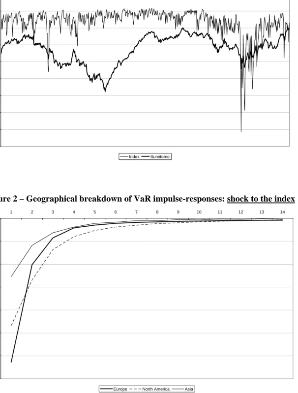
Table 2 reports as an example the estimation results for the Sumitomo Mitsui Fi-nancial Group, the second largest bank in Japan by market value (as of November

2009). Notice that the non-diagonal coe¢ cients for the B matrix are signi…cantly

di¤erent from zero, illustrating how the multivariate quantile model can uncover dynamics that cannot be detected by estimating univariate quantile models. In general, we reject the joint null hypothesis that all o¤-diagonal coe¢ cients of the

matrices A and B are equal to zero at the .05 level [**HW: correct level?]

for the index and the Sumitomo Mitsui Financial Group are reported in Figure 1. The quantile of the global index is generally much smaller in absolute terms that the quantile of Sumitomo, re‡ecting the portfolio diversi…cation e¤ect of the index. Only around the Lehman bankruptcy (September 2008) is the situation brie‡y inverted, with the estimates indicating a higher risk associated with the global index than with the Sumitomo bank.

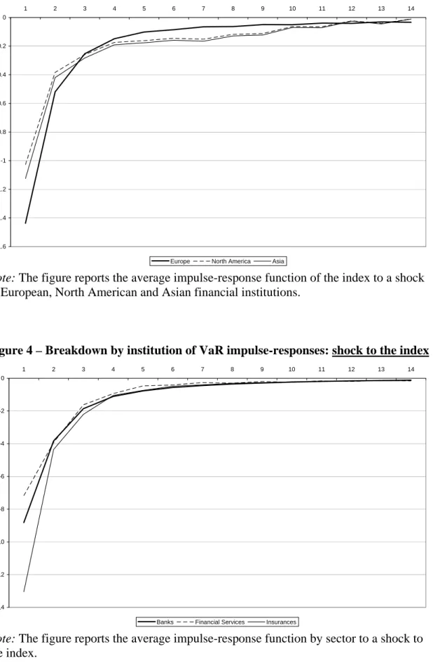
Figures 2-5 plot the average impulse-response functions@q1;t+n=@u2;tand@q2;t+n

=@u1;t measuring the impact of a two standard deviation individual bank shock

on the index and the impact of a two standard deviation shock to the index on the individual bank’s risk. In Figures 2 and 3, the average is taken with respect to the geographical distribution. That is, the average impulse-response for Europe, say, is obtained by averaging all the impulse-response functions for European …nancial institutions. We notice two things. First, the impact of a shock to the index is much stronger than the impact of a shock to the individual …nancial institution. This result is partly driven by our identi…cation assumption that shocks to the index have a contemporaneous impact on the return of the single …nancial institutions, while the institution’s speci…c shocks have only a lagged impact on the global …nancial index. Second, we notice that the risk of Asian …nancial institutions appears to be on average much less sensitive to global shocks than their European and North American counterparts.

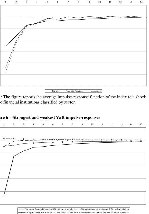
Figures 4 and 5 plot the average impulse-response functions for the …nancial institutions grouped by line of business, i.e. banks, …nancial services, and insur-ances. We see that a shock to the index has a stronger initial impact on the group of insurance companies. Regarding the impact of shocks to the individual …nancial institutions on the risk of the global index, banks have on average a lower initial impact, but the shock appears to be more persistent than for …nancial services and insurance companies.

To rank the …nancial institutions according to their impact on risk, we inte-grated out all the individual impulse-responses and sorted the …nancial institutions according to this metric. The resulting ranking is reported in Table 3. The …rst two columns rank the 20 …nancial institutions whose risk is most and least sensi-tive to a shock to the index. Among the most sensisensi-tive institutions are household names such as Barclays, Unicredit, Citigroup, and Royal Bank of Scotland. Gold-man Sachs, on the other hand, belongs to the group of …nancial institutions that are least a¤ected by global shocks. The last two columns contain the …nancial institutions with the largest and smallest impact on the risk of the global index. These lists contain smaller and less well known …nancial institutions. To get an idea of the orders of magnitude involved, Figure 6 plots the average impulse-responses corresponding to the four lists of 20 …nancial institutions contained in Table 3. It is clear that the shocks to the index have an impact of an order of magnitude greater than the shocks to the individual …nancial institutions. A two standard deviation shock to the index produces an average initial increase in the VaR of the most sensitive …nancial institutions of more than 20%. The shock is also quite persistent, as it is not yet completely absorbed after 15 weeks. On the other hand, for the least sensitive …nancial institutions, a shock to the index

produces an average immediate increase in the VaR of less than 3%, which is then entirely absorbed after the second week. The …gure also shows that the shocks to the individual …nancial institutions have a signi…cantly lower impact on the risk of the index, in line with the results shown in Figures 3 and 5.

5

Conclusion

We have developed theory ensuring the consistency and asymptotic normality of multivariate multi-quantile models. Our theory is general enough to comprehen-sively cover models with multiple random variables, multiple con…dence levels and multiple lags of the quantiles.

We conduct an empirical analysis in which we estimate a VAR for VaR model using returns of individual …nancial institutions from around the world and a global …nancial sector index. By examining the impulse-response functions, we can rank the banks by their resilience to shocks to the overall index and by the impact they have on the VaR of the …nancial sector index. We …nd that the risk of Asian …nancial institutions tends to be less sensitive to systemic shocks, whereas insurance companies exhibit a greater sensitivity to global shocks. Ranking …nan-cial institutions by how they react to shocks, we uncover wide di¤erences among them. Among the top 20 …nancial institutions that appear to be more vulnera-ble to system-wide shocks we …nd well-known names such as Barclays, Unicredit, Citigroup, and Royal Bank of Scotland. These …ndings are quite striking, as they are obtained without weighting the …nancial institutions by their market capital-ization.

The methods developed in this paper can be applied to many other contexts. For instance, many stress-test models are built from vector autoregressive models on credit risk indicators and macroeconomic variables. Starting from the estimated mean and adding assumptions on the multivariate distribution of the error terms, one can deduce the impact of a macro shock on the quantile of the credit risk variables. Our methodology provides a convenient alternative for stress testing, by allowing researchers to estimate vector autoregressive processes directly on the quantiles of interest, rather than on the mean.

References

[1] Acharya, V., Pedersen, L., Philippe, T., and Richardson, M. (2010). Measur-ing systemic risk. Technical report, Department of Finance, NYU.

[2] Adrian, T. and Brunnermeier, M. (2009). CoVaR. Manuscript, Princeton Uni-versity.

[3] Andersen, T. G., Bollerslev, T., Diebold, F. X. and Labys, P. (2003). Modeling

[4] Andrews, D.W.K. (1988). Laws of large numbers for dependent

non-identically distributed random variables. Econometric Theory 4, 458-467.

[5] Bartle, R. (1966).The Elements of Integration. New York: Wiley.

[6] Engle, R.F. and C.T. Brownlees (2010). Volatility, Correlation and Tails for Systemic Risk Measurement. Manuscript, Stern School of Business, New York University.

[7] Engle, R.F. and Manganelli, S. (2004). CAViaR: Conditional autoregressive

value at risk by regression quantiles. Journal of Business & Economic

Statis-tics 22, 367-381.

[8] Huber, P.J. (1967). The behavior of maximum likelihood estimates under

non-standard conditions. Proceedings of the Fifth Berkeley Symposium on

Math-ematical Statistics and Probability. Berkeley: University of California Press, pp. 221–233.

[9] Kim, T.-H. and White, H. (2003). Estimation, inference, and speci…cation testing for possibly misspeci…ed quantile regression. In T. Fomby and C. Hill,

eds., Maximum Likelihood Estimation of Misspeci…ed Models: Twenty Years

Later. New York: Elsevier, pp. 107-132.

[10] Koenker, R. and Bassett, G. (1978). Regression quantiles. Econometrica 46,

33–50.

[11] Komunjer, I. (2005). Quasi-maximum likelihood estimation for conditional

quantiles. Journal of Econometrics 128, 127-164.

[12] Komunjer, I. and Vuong, Q. (2006). E¢ cient conditional quantile estima-tion: the time series case. University of California, San Diego Department of Economics Discussion Paper 2006-10, .

[13] Komunjer, I. and Vuong, Q. (2007a). Semiparametric e¢ ciency bound and M-estimation in time-series models for conditional quantiles. University of California, San Diego Department of Economics Discussion Paper

[14] Komunjer, I. and Vuong, Q. (2007b). E¢ cient estimation in dynamic con-ditional quantile models. University of California, San Diego Department of Economics Discussion Paper.

[15] Newey, W.K. and Powell, J.L. (1990). E¢ cient estimation of linear and type

I censored regression models under conditional quantile restrictions.

Econo-metric Theory 6, 295-317.

[16] Otsu, T. (2003). Empirical likelihood for quantile regression. University of Wisconsin, Madison Department of Economics Discussion Paper.

[17] Powell, J. (1984). Least absolute deviations estimators for the censored

[18] Stinchcombe, M. and White, H. (1998). Consistent speci…cation testing with

nuisance parameters present only under the alternative.Econometric Theory

14, 295-324.

[19] Weiss, A. (1991). Estimating nonlinear dynamic models using least absolute

error estimation. Econometric Theory 7, 46-68.

[20] White, H. (1994). Estimation, Inference and Speci…cation Analysis. New

York: Cambridge University Press.

[21] White, H. (2001). Asymptotic Theory for Econometricians. San Diego:

Aca-demic Press.

[22] White, H. (2006). Approximate nonlinear forecasting methods. In G. Elliott,

C.W.J. Granger, and A. Timmermann, eds.,Handbook of Economic

Forecast-ing. New York: Elsevier, pp. 460-512.

[23] White, H., Kim, T.-H., and Manganelli, S. (2008). Modeling autoregressive conditional skewness and kurtosis with multi-quantile CAViaR. In J. Russell

and M. Watson, eds.,Volatility and Time Series Econometrics: A Festschrift

in Honor of Robert F. Engle, forthcoming.

6

Appendix 1 - Multi-quantile representation of

a bivariate GARCH process with zero mean

Y1t Y2t = t 0 t t "1t "2t "tvN(0; I) t(Y1t) = t 1t = c1+a11jY1t 1j+a12jY2t 1j+b11 1t 1+b12 2t 1 t(Y2t) = q 2 t + 2t 2t = c2+a21jY1t 1j+a22jY2t 1j+b21 1t 1+b22 2t 1:

The respective quantile processes are:

q1t = kc1+ka11jY1t 1j+ka12jY2t 1j+b11q1t 1+b12q2t 1

q2t = kc2+ka21jY1t 1j+ka22jY2t 1j+b21q1t 1+b22q2t 1;

wherekis the -quantile of the standard normal distribution. In this case, setting

the shocks equal to zero is equivalent to setting Yt = 0. The long-run quantiles

are: q = 1 b11 b12 b21 1 b22 1 kc1 kc2

7

Appendix 2 - Proofs

The proofs that follow are straightforward modi…cations of those in White, Kim, and Manganelli (2008).

We establish the consistency of ^T by applying results of White (1994). For

this we impose the following moment and domination conditions. In stating this next condition and where convenient elsewhere, we exploit stationarity to omit

explicit reference to all values of t:

Assumption 5(i) Fori= 1; :::; n; E_jYitj<1;(ii) letD0;t := maxi=1;:::;nmaxj=1;:::;p

sup _2Ajqi;j;t(; )j: ThenE(D0;t)<1:

Proof of Theorem 1: We verify the conditions of corollary 5.11 of White (1994),

which delivers ^T ! , where

^T := arg max 2A T 1 T X t=1 '_t(Yt; qt(; )); and '_t(Yt; qt(; )) := f Pn i=1 Pp

j=1 ij(Yit qi;j;t(; ))g. Assumption 1 ensures

White’s Assumption 2.1. Assumption 3(i) ensures White’s Assumption 5.1. Our

choice of _ij satis…es White’s Assumption 5.4. To verify White’s Assumption 3.1,

it su¢ ces that '_t(Yt; qt(; )) is dominated on A by an integrable function

(en-suring White’s Assumption 3.1(a,b)) and that for each in _A, _f'_t(Yt; qt(; ))g

is stationary and ergodic (ensuring White’s Assumption 3.1(c), the strong uni-form law of large numbers (ULLN)). Stationarity and ergodicity is ensured by Assumptions 1 and 3(i). To show domination, we write

j'_t(Yt; qt(; ))j n X i=1 p X j=1 j ij(Yit qi;j;t(; ))j = n X i=1 p X j=1 j(Yit qi;j;t(; ))( ij 1[Yit qi;j;t(; ) 0])j 2 n X i=1 p X j=1 (_jYitj+jqi;j;t(; )j) 2p n X i=1 jYitj+ 2npjD0;tj; so that sup 2A j '_t(Yt; qt(; ))j 2p n X i=1 jYitj+ 2npjD0;tj:

Thus,2pPn_i=1jYitj+ 2npjD0;tjdominates j't(Yt; qt(; ))j; this has …nite

expecta-tion by Assumpexpecta-tion 5(i,ii).

It remains to verify White’s Assumption 3.2; here this is the condition that

4(i), it follows by argument directly parallel to that in the proof of White (1994,

corollary 5.11) that for all _2A;

E('_t(Yt; qt(; )) E('t(Yt; qt(; )):

Thus, it su¢ ces to show that the above inequality is strict for ₆= : Consider

6

= such that _{jj jj} > and let ( ) := Pn_i=1Pp_j=1E( i;j;t( )) with

i;j;t( ) := ij(Yit qi;j;t(; )) ij(Yit qi;j;t(; )): It will su¢ ce to show that ( ) >0: First, we de…ne the "error" "i;j;t := Yit qi;j;t(; ) and let fi;j;t( ) be

the density of "i;j;t conditional on Ft 1: Noting that i;j;t( ; ) := qi;j;t(; )

qi;j;t(; );we next can show by some algebra and Assumption2(ii.a) that

E( i;j;t( )) = E[ Z i;j;t( ; ) 0 ( i;j;t( ; ) s) fi;j;t(s)ds] E[1 2 2₁ [ji;j;t( ; )j> ]+ 1 2 i;j;t( ; ) 2₁ [j i;j;t( ; )j ])] 1 2 2_E[1 [ji;j;t( ; )j> ]]:

The …rst inequality above comes from the fact that Assumption 2(ii.a) implies

that for any >0 su¢ ciently small, we have fi;j;t(s)> for jsj< . Thus,

( ) : = n X i=1 p X j=1 E( i;j;t( )) 1 2 2 n X i=1 p X j=1 E[1[ji;j;t( ; )j> ]] = 1 2 2 n X i=1 p X j=1 P[_j i;j;t( ; )j> ] 1 2 2 X (i;j)2I P[_j i;j;t( ; )j> ] 1 2 2_P[ [(i;j)2Ifj i;j;t( ; )j> g]>0;

where the …nal inequality follows from Assumption 4(i.b). As is arbitrary, the

result follows.

Next, we establish the asymptotic normality ofT1=2(^T ). We use a method

originally proposed by Huber (1967) and later extended by Weiss (1991). We …rst sketch the method before providing formal conditions and the proof.

Huber’s method applies to our estimator ^T; provided that ^T satis…es the

asymptotic …rst order conditions

T 1 T X t=1 f n X i=1 p X j=1 rqi;j;t(;^T) _ij(Yit qi;j;t(;^T))g=op(T1=2); (8)

where_rqi;j;t(; )is the ` 1gradient vector with elements(@=@ s)qi;j;t(; ); s=

1; :::; `; and _ij(Yit qi;j;t(;^T)) is a generalized residual. Our …rst task is thus

to ensure that eq. (8) holds. Next, we de…ne ( ) := n X i=1 p X j=1 E[_rqi;j;t(; ) _ij(Yit qi;j;t(; ))]:

With ( )continuously di¤erentiable at interior to_A, we can apply the mean value theorem to obtain

( ) = ( ) +Q0( ); (9)

whereQ0 is an` `matrix with(1 `)rowsQ0;s =r0 ( (s)), where (s)is a mean

value (di¤erent for each s) lying on the segment connecting and ; s= 1; :::; `.

It is straightforward to show that correct speci…cation ensures that ( )is zero.

We will also show that

Q0 = Q +O(jj jj); (10)

where Q :=Pn_i=1Pp_j=1E[fi;j;t(0)rqi;j;t(; )r0qi;j;t(; )]with fi;j;t(0) the value

at zero of the density fi;j;t of "i;j;t :=Yit qi;j;t(; ); conditional on Ft 1:

Com-bining eqs. (9) and (10) and putting ( ) = 0, we obtain

( ) = Q ( ) +O(_{jj jj}2): (11)

The next step is to show that

T1=2 (^T) +HT =op(1); (12) where HT := T 1=2 PT t=1 t; with t := Pn i=1 Pp

j=1rqi;j;t(; ) ij("i;j;t). Eqs.

(11) and (12) then yield the following asymptotic representation of our estimator

^T: T1=2(^T ) = Q 1T 1=2 T X t=1 t +op(1): (13)

As we impose conditions su¢ cient to ensure that _f t;Ftg is a martingale

dif-ference sequence (MDS), a suitable central limit theorem (e.g., theorem 5.24 in

White, 2001) applies to eq. (13) to yield the desired asymptotic normality of ^T:

T1=2(^T ) d

!N(0; Q 1V Q 1); (14)

where V :=E( _t 0

t ).

We now strengthen the conditions above to ensure that each step of the above argument is valid.

Assumption 2 (iii) (a) There exists a …nite positive constant f0 such that for

each i and t; each ! ₂ ; and each y_{2 R}, fit(!; y) f0 <1; (b) There exists a

…nite positive constantL0 such that for eachiandt;each! 2 ;and eachy1; y2 2

R, _jfit(!; y1) fit(!; y2)j L0jy1 y2j.

Next we impose su¢ cient di¤erentiability ofqt with respect to .

Assumption 3 (ii) For each t and each ! ₂ ; qt(!; ) is continuously

di¤er-entiable on _A; (iii) For each t and each ! ₂ ; qt(!; ) is twice continuously

To exploit the mean value theorem, we require that belongs to int(_A), the interior of _A.

Assumption 4 (ii) ₂int(_A):

Next, we place domination conditions on the derivatives of qt:

Assumption 5 (iii) LetD1;t := maxi=1;:::;nmaxj=1;:::;pmaxs=1;:::;`sup _2Aj(@=@ s)

qi;j;t(; )j. Then (a) E(D1;t) < 1; (b) E(D21;t) < 1; (iv) Let D2;t :=

maxi=1;:::;nmaxj=1;:::;pmaxs=1;:::;`maxh=1;:::;`sup _2Aj(@2=@ s@ h)qi;j;t(; )j. Then

(a)E(D2;t)<1; (b)E(D22;t)<1:

Assumption 6(i)Q :=Pn_i=1Pp_j=1E[fi;j;t(0)rqi;j;t(; )r0qi;j;t(; )]is positive

de…nite; (ii) V :=E( _t 0

t) is positive de…nite.

Assumptions3(ii) and5(iii.a) are additional assumptions helping to ensure that eq.

(8) holds. Further imposing Assumptions 2(iii), 3(iii.a), 4(ii), and 5(iv.a) su¢ ces

to ensure that eq. (11) holds. The additional regularity provided by Assumptions

5(iii.b), 5(iv.b), and 6(i) ensures that eq. (12) holds. Assumptions 5(iii.b) and

6(ii) help ensure the availability of the MDS central limit theorem.

We now have conditions su¢ cient to prove asymptotic normality of our MVMQ-CAViaR estimator.

Proof of Theorem 2: As outlined above, we …rst prove

T 1 T X t=1 f n X i=1 p X j=1 rqi;j;t(;^T) ij(Yit qi;j;t(;^T))g=op(1): (15)

The existence of _rqi;j;t is ensured by Assumption 3(ii). Let ei be the ` 1 unit

vector with ith _{element equal to one and the rest zero, and let}

Gs(c) := T 1=2 T X t=1 n X i=1 p X j=1 ij(Yit qi;j;t(;^T +ces));

for any real numberc. Then by the de…nition of ^T,Gs(c) is minimized atc= 0.

LetHs(c) be the derivative ofGs(c) with respect toc from the right. Then

Hs(c) = T 1=2 T X t=1 n X i=1 p X j=1 rsqi;j;t(;^T +ces) _ij(Yit qi;j;t(;^T +ces));

where _rsqi;j;t(;^T +ces)is the sth element of rqi;j;t(;^T +ces). Using the facts

that (i) Hs(c) is non-decreasing in c and (ii) for any > 0, Hs( ) 0 and

Hs( ) 0, we have jHs(0)j Hs( ) Hs( ) T 1=2 T X t=1 n X i=1 p X j=1 jrsqi;j;t(;^T)j1[Yit qi;j;t(;^T)=0] T 1=2 max 1 t TD1;t T X t=1 n X i=1 p X j=1 1[Yit qi;j;t(;^T)=0];

where the last inequality follows by the domination condition imposed in Assump-tion 5(iii.a). Because D1;t is stationary, T 1=2max1 t TD1;t =op(1). The second

term is bounded in probability: PT_t=1Pn_i=1Pp_j=11[Yit qi;j;t(;^T)=0] = Op(1) given

Assumption 2(i,ii.a) (see Koenker and Bassett, 1978, for details). Since Hs(0) is

the sth element of T 1=2P_tT₌₁Pn_i=1Pp_j=1rqi;j;t(;^T) ij(Yit qi;j;t(;^T)), the

claim in (15) is proved.

Next, for each _{2 A}, Assumptions 3(ii) and 5(iii.a) ensure the existence and

…niteness of the` 1vector

( ) : = n X i=1 p X j=1 E[_rqi;j;t(; ) ij(Yit qi;j;t(; ))] = n X i=1 p X j=1 E[_rqi;j;t(; ) Z 0 i;j;t( ; ) fi;j;t(s)ds];

where i;j;t( ; ) :=qi;j;t(; ) qi;j;t(; )and fi;j;t(s) = (d=ds)Fit(s+qi;j;t(; ))

represents the conditional density of "i;j;t := Yit qi;j;t(; ) with respect to

Lebesgue measure: The di¤erentiability and domination conditions provided by

Assumptions 3(iii) and 5(iv.a) ensure (e.g., by Bartle, 1966, corollary 5.9) the

continuous di¤erentiability of ( ) on_A, with

r ( ) = n X i=1 p X j=1 E[_rfr0qi;j;t(; ) Z 0 i;j;t( ; ) fi;j;t(s)dsg]:

Since is interior to_A by Assumption 4(ii), the mean value theorem applies to

each element of ( )to yield

( ) = ( ) +Q0( ); (16)

for in a convex compact neighborhood of where Q0 is an ` ` matrix with

(1 `) rows Qs( (s)) = r0 ( (s)), where (s) is a mean value (di¤erent for each

s) lying on the segment connecting and with s= 1; :::; `. The chain rule and

an application of the Leibniz rule to R0

i;j;t( ; )fi;j;t(s)ds then give

Qs( ) =As( ) Bs( ); where As( ) := n X i=1 p X j=1 E[_rsr0qi;j;t(; ) Z 0 i;j;t( ; ) fi;j;t(s)ds] Bs( ) := n X i=1 p X j=1

E[fi;j;t( i;j;t( ; ))rsqi;j;t(; )r0qi;j;t(; )]:

Assumption 2(iii) and the other domination conditions (those of Assumption 5)

then ensure that

As( (s)) = O(jj jj)

whereQ_s :=Pn_i=1P_jp₌₁E[fi;j;t(0)rsqi;j;t(; )r0qi;j;t(; )]:LettingQ :=Pn_i=1Pp_j=1

E[fi;j;t(0)rqi;j;t(; )r0qi;j;t(; )], we obtain

Q0 = Q +O(jj jj): (17)

Next, we have that ( ) = 0: To show this, we write

( ) = n X i=1 p X j=1 E[_rqi;j;t(; ) ij(Yit qi;j;t(; ))] = n X i=1 p X j=1 E(E[_rqi;j;t(; ) ij(Yit qi;j;t(; ))j Ft 1]) = n X i=1 p X j=1 E(_rqi;j;t(; )E[ ij(Yit qi;j;t(; ))j Ft 1]) = n X i=1 p X j=1 E(_rqi;j;t(; )E[ ij("i;j;t)j Ft 1]) = 0;

as E[ _ij("i;j;t) j Ft 1] = ij E[1[Yit qi;j;t] j Ft 1] = 0; by de…nition of qi;j;t for

i= 1; :::; n and j = 1; :::; p (see eq. (3)). Combining ( ) = 0 with eqs. (16) and (17), we obtain

( ) = Q ( ) +O(_{jj jj}2): (18)

The next step is to show that

T1=2 (^T) +HT =op(1) (19) whereHT :=T 1=2 PT t=1 t;with t := t( )and t( ) := Pn i=1 Pp j=1rqi;j;t(; )

ij(Yit qi;j;t(; )). Letut( ; d) := supf :jj jj dgjj t( ) t( )jj. By the results

of Huber (1967) and Weiss (1991), to prove (19) it su¢ ces to show the following: (i)

there exista >0and d0 >0such thatjj ( )jj ajj jjforjj jj d0; (ii)

there existb >0; d0 >0;andd 0such thatE[ut( ; d)] bdforjj jj+d d0;

and (iii) there exist c > 0; d0 > 0; and d 0 such that E[ut( ; d)2] cd for

jj jj+d d0.

(i). For (ii), we have that for given (small)d >0 ut( ; d) sup f :jj jj dg n X i=1 p X j=1

jjrqi;j;t(; ) ij(Yit qi;j;t(; )) rqi;j;t(; ) ij(Yit qi;j;t(; ))jj

n X i=1 p X j=1 sup f :jj jj dgjj ij (Yit qi;j;t(; ))jj sup f :jj jj dgjjr qi;j;t(; ) rqi;j;t(; )jj + n X i=1 p X j=1 sup f :jj jj dgjj ij (Yit qi;j;t(; )) ij(Yit qi;j;t(; ))jj sup f :jj jj d_gjjr qi;j;t(; )jj npD2;td+D1;t n X i=1 p X j=1 1[jYit qi;j;t(; )j<D1;td]

using the following: (i) _{jj ij}(Yit qi;j;t(; ))jj 1; (ii) jj ij(Yit qi;j;t(; )) ij(Yit qi;j;t(; ))jj 1[jYit qi;j;t(; )j<jqi;j;t(; ) qi;j;t(; )j]; and (iii) the mean value

theorem applied to_rqi;j;t(; ) and qi;j;t(; ). Hence, we have

E[ut( ; d)] npC0d+ 2npC1f0d

for some constants C0 and C1; given Assumptions 2(iii.a), 5(iii.a), and 5(iv.a).

Hence, (ii) holds for b = npC0 + 2npC1f0 and d0 = 2d: The last condition (iii)

can be similarly veri…ed by applying thecr inequality to eq. (??) withd <1(so

that d2 _{< d) and using Assumptions 2(iii.a), 5(iii.b), and5(iv.b). Thus, eq. (19)}

is veri…ed.

Combining eqs. (18) and (19) thus yields

Q T1=2(^T ) =T 1=2 T

X

t=1

t +op(1):

But_{f t};_Ftgis a stationary ergodic martingale di¤erence sequence (MDS). In

par-ticular, _t is measurable _Ft, andE( tjFt 1) = E(

Pn i=1 Pp j=1rqi;j;t(; ) ij("i;j;t) j Ft 1) = Pn i=1 Pp

j=1rqi;j;t(; )E( ij("i;j;t) j Ft 1) = 0, as E[ ij("i;j;t) j

Ft 1] = 0 for all i = 1; :::; n and j = 1; :::; p: Assumption 5(iii.b) ensures that

V := E( _t 0

t) is …nite. The MDS central limit theorem (e.g., theorem 5.24 of

White, 2001) applies, provided V is positive de…nite (as ensured by

Assump-tion 6(ii)) and thatT 1PT

t=1 t t0 =V +op(1), which is ensured by the ergodic

theorem. The standard argument now gives

V 1=2Q T1=2(^T ) d

!N(0; I);

Proof of Theorem 3: We have ^ VT V = (T 1 T X t=1 ^_t^0_t T 1 T X t=1 t t0) + (T 1 T X t=1 t t0 E[ t t0]);

where^_t:=Pn_i=1P_jp_=1rq^i;j;t^i;j;tand t :=

Pn i=1

Pp

j=1rqi;j;t i;j;t;withrq^i;j;t:=

rqi;j;t(;^T);^i;j;t := ij(Yit qi;j;t(;^T));rqi;j;t := rqi;j;t(; ), and i;j;t := ij(Yit qi;j;t(; )):Assumptions1and 2(i,ii) ensure thatf t

0

tgis a stationary

ergodic sequence. Assumptions3(i,ii),4(i.a), and 5(iii) ensure thatE[ _t 0

t ]<1:

It follows by the ergodic theorem that T 1PT

t=1 t t0 E[ t t0] =op(1):Thus, it

su¢ ces to proveT 1PT

t=1^t^0t T 1 PT t=1 t t0 =op(1): The (h; s) element of T 1PT t=1^t^0t T 1 PT t=1 t t0 is T 1 T X t=1 f n X i=1 p X j=1 n X l=1 p X k=1

(^_i;j;t^_l;k;trhq^i;j;trsq^l;k;t i;j;t l;k;trhqi;j;trsql;k;t)g:

Thus, it will su¢ ce to show that for each (h; s) and (i; j; l; k),

T 1

T

X

t=1

f^i;j;t^l;k;trhq^i;j;trsq^l;k;t i;j;t l;k;trhqi;j;trsql;k;tg=op(1):

By the triangle inequality,

jT 1

T

X

t=1

f^i;j;t^l;k;trhq^i;j;trsq^l;k;t i;j;t l;k;trhqi;j;trsql;k;tgj AT +BT;

where

AT = T 1 T

X

t=1

j^i;j;t^l;k;trhq^i;j;trsq^l;k;t i;j;t l;k;trhq^i;j;trsq^l;k;tj

BT = T 1 T

X

t=1

j i;j;t l;k;trhqi;j;trsql;k;t i;j;t l;k;trhq^i;j;trsq^l;k;tj:

We now show that AT = op(1) and BT = op(1), delivering the desired result.

ForAT;the triangle inequality gives

AT A1T +A2T +A3T; where A1T = T 1 T X t=1

ijj1["i;j;t 0] 1[^"i;j;t 0]jjrhq^i;j;trsq^l;k;tj

A2T = T 1 T X t=1 lkj1["l;k;t 0] 1[^"l;k;t 0]jjrhq^i;j;trsq^l;k;tj A3T = T 1 T X t=1

Theorem 2, ensured by Assumptions 1 6, implies that T1=2

jj^T jj=Op(1):

This, together with Assumptions2(iii,iv) and5(iii.b), enables us to apply the same

techniques used in Kim and White (2003) to showA1T =op(1), A2T =op(1); and

A3T =op(1), implyingAT =op(1):

It remains to show BT =op(1). By the triangle inequality,

BT B1T +B2T; where B1T = T 1 T X t=1

j i;j;t l;k;trhqi;j;trsql;k;t E[ i;j;t l;k;trhqi;j;trsql;k;t]j

B2T = T 1 T

X

t=1

j i;j;t l;k;trhq^i;j;trsq^l;k;t E[ i;j;t l;k;trhqi;j;trsql;k;t]j:

Assumptions 1, 2(i,ii), 3(i,ii), 4(i.a), and 5(iii) ensure that the ergodic theorem

applies to _{f i;j;t l;k;tr}hqi;j;trsql;k;tg;so B1T =op(1):Next, Assumptions 1,3(i,ii),

and5(iii) ensure that the stationary ergodic ULLN applies to_f i;j;t l;k;trhqi;j;t(; )

rsql;k;t(; )g: This and the result of Theorem 1 (^T = op(1)) ensure that

B2T =op(1) by e.g., White (1994, corollary 3.8), and the proof is complete.

To establish consistency of Q^T; we strengthen the domination condition on

rqi;j;t and impose conditions on f^cTg.

Assumption 5 (iii.c) E(D3

1;t)<1:

Assumption 7_f^cTgis a stochastic sequence andfcTgis a non-stochastic sequence

such that (i) ^cT=cT p

!1; (ii) cT =o(1); and (iii) cT1 =o(T1=2).

Proof of Theorem 4: We begin by sketching the proof. We …rst de…ne

QT := (2cTT) 1 T X t=1 n X i=1 p X j=1 1[ cT "i;j;t cT]rqi;j;tr 0_q i;j;t;

and then we will show the following:

Q E(QT) p !0; (20) E(QT) QT p !0; (21) QT Q^T p !0: (22)

Combining the results above will deliver the desired outcome: Q^T Q

p

!0.

For (20), one can show by applying the mean value theorem to Fi;j;t(cT)

Fi;j;t( cT), where Fi;j;t(c) :=

R 1_fs cgfi;j;t(s)ds, that E(QT) =T 1 T X t=1 n X i=1 p X j=1

E[fi;j;t( i;j;T)rqi;j;tr0qi;j;t] = n X i=1 p X j=1

where _i;j;T is a mean value lying between cT and cT; and the second equality

follows by stationarity. Therefore, the (h; s)element of _jE(QT) Q j satis…es

j n X i=1 p X j=1

E_ffi;j;t( i;j;T) fi;j;t(0)rhqi;j;trsqi;j;tgj

n X i=1 p X j=1

E_fjfi;j;t( i;j;T) fi;j;t(0)jjrhqi;j;trsqi;j;tjg

n X i=1 p X j=1

L0Efj i;j;Tjjrhqi;j;trsqi;j;tjg

npL0cTE[D21;t];

which converges to zero as cT !0. The second inequality follows by Assumption

2(iii.b), and the last inequality follows by Assumption 5(iii.b). Therefore, we have the result in eq.(20).

To show (21), it su¢ ces simply to apply a LLN for double arrays, e.g. theorem 2 in Andrews (1988).

Finally, for (22), we consider the (h; s)element of _jQ^T QTj, given by

j 1 2^cTT T X t=1 n X i=1 p X j=1

1[ ^cT ^"i;j;t ^cT]rhq^i;j;trsq^i;j;t

1 2cTT T X t=1 n X i=1 p X j=1

1[ cT "i;j;t cT]rhqi;j;trsqi;j;tj

= cT ^ cT j 1 2cTT T X t=1 n X i=1 p X j=1

(1[ ^cT ^"i;j;t c^T] 1[ cT "i;j;t cT])rhq^i;j;trsq^i;j;t

+ 1 2cTT T X t=1 n X i=1 p X j=1

1[ cT "i;j;t cT](rhq^i;j;t rhqi;j;t)rsq^i;j;t

+ 1 2cTT T X t=1 n X i=1 p X j=1

1[ cT "i;j;t cT]rhqi;j;t(rsq^i;j;t rsqi;j;t)

+ 1 2cTT (1 c^T cT ) T X t=1 n X i=1 p X j=1

1[ cT "i;j;t cT]rhqi;j;trsqi;j;tj

cT ^ cT [A1T +A2T +A3T + (1 ^ cT cT )A4T];

where A1T := 1 2cTT T X t=1 n X i=1 p X j=1

j1[ ^cT ^"i;j;t ^cT] 1[ cT "i;j;t cT]j jrhq^i;j;trsq^i;j;tj

A2T := 1 2cTT T X t=1 n X i=1 p X j=1

1[ cT "i;j;t cT]jrhq^i;j;t rhqi;j;tj jrsq^i;j;tj

A3T := 1 2cTT T X t=1 n X i=1 p X j=1

1[ cT "i;j;t cT]jrhqi;j;tj jrsq^i;j;t rsqi;j;tj

A4T := 1 2cTT T X t=1 n X i=1 p X j=1

1[ cT "i;j;t cT]jrhqi;j;trsqi;j;tj:

It will su¢ ce to show that A1T = op(1); A2T = op(1); A3T = op(1); and A4T =

Op(1): Then, becausec^T=cT p

!1, we obtain the desired result: Q^T Q

p

!0.

We …rst show A1T =op(1). It will su¢ ce to show that for each i and j,

1 2cTT

T

X

t=1

j1[ ^cT ^"i;j;t c^T] 1[ cT "i;j;t cT]j jrhq^i;j;trsq^i;j;tj=op(1):

Let T lie between ^T and ; and put di;j;t;T :=jjrqi;j;t(; T)jj jj^T jj+

j^cT cTj: Then

(2cTT) 1 T

X

t=1

j1[ ^cT ^"i;j;t c^T] 1[ cT "i;j;t cT]j jrhq^i;j;trsq^i;j;tj UT +VT;

where

UT := (2cTT) 1

T

X

t=1

1[j"i;j;t cTj<di;j;t;T]jrhq^i;j;trsq^i;j;tj

VT := (2cTT) 1

T

X

t=1

1[j"i;j;t+cTj<di;j;t;T]jrhq^i;j;trsq^i;j;tj:

It will su¢ ce to show thatUT

p

!0andVT

p

!0:Let >0and letz be an arbitrary

positive number. Then, using reasoning similar to that of Kim and White (2003,

lemma 5), one can show that for any >0;

P(UT > ) P((2cTT) 1 T

X

t=1

1[j"i;j;t cTj<(jjrqi;j;t(; T)jj+1)zcT])jrhq^i;j;trsq^i;j;tj> )

zf0 T T X t=1 E_f(_jjrqi;j;t(; T)jj+ 1)jrhq^j;trsq^j;tjg zf0fEjD31;tj+EjD 2 1;tjg= ;

where the second inequality is due to the Markov inequality and Assumption

2(iii.a), and the third is due to Assumption 5(iii.c). Asz can be chosen arbitrarily

small and the remaining terms are …nite by assumption, we have UT

p

! 0. The

same argument is used to showVT

p

!0: Hence, A1T =op(1) is proved.

Next, we showA2T =op(1). For this, it su¢ ces to showA2T;i;j := _2c1_TT

PT t=1

1[ cT "i;j;t cT]jrhq^i;j;t rhqi;j;tj jrsq^i;j;tj=op(1) for eachi and j. Note that

A2T;i;j 1 2cTT T X t=1

jrhq^i;j;t rhqi;j;tj jrsq^i;j;tj

1 2cTT T X t=1 jjr2hqi;j;t(;~)jj jj^T jj jrsq^i;j;tj 1 2cTjj ^T jj 1 T T X t=1 D2;tD1;t = 1 2cTT1=2 T1=2_jj^T jj 1 T T X t=1 D2;tD1;t;

where ~ is between ^T and , and r2hqj;t(;~) is the …rst derivative of rhq^j;t

with respect to ; which is evaluated at ~. The last expression above is op(1)

because: (i)T1=2

jj^T jj=Op(1) by Theorem 2; (ii)T 1

PT

t=1D2;tD1;t =Op(1)

by the ergodic theorem; and (iii)1=(cTT1=2) =op(1) by Assumption 7(iii). Hence,

A2T =op(1). The other claims A3T =op(1) and A4T =Op(1) can be analogously

and more easily proven. Hence, they are omitted. Therefore, we …nally have

QT Q^T p

! 0; which, together with (20) and (21), implies that Q^T Q

p

! 0.

Table 1 – Breakdown of financial institutions by sector and by geographic area

Banks Financial Services Insurances

EU 47 22 27 96

North America 25 17 28 70

Asia 47 14 3 64

119 53 58 230

Note: Classification as provided by Datastream. Swiss and Norwegian financial institutions have been classified as EU. Asia includes Australian financial institutions.

Table 2 – Estimates and standard errors for the Sumitomo Mitsui Financial Group

1 c a₁₁ a₁₂ b₁₁ b₁₂ -2.71 -0.89 -0.13 0.61 -0.11 s.e. 1.48 0.37 0.13 0.12 0.06 2 c a₂₁ a₂₂ b₂₁ b₂₂ -1.05 0.07 -0.12 -0.08 0.93 s.e. 0.48 0.10 0.05 0.04 0.03

Table 3 – Ranking of financial institutions according to impulse responses Financial institutions most sensitive to index’s shocks Financial institutions least sensitive to index’s shocks Financial institutions with greatest impact on

index VaR

Financial institutions with lowest impact on

index’s risk

1 ING GROEP WESTPAC BANKING WESTPAC BANKING SWISS RE 'R' 2 BARCLAYS CHINA EVERBRIGHT SLM UNICREDIT 3 UNICREDIT CREDITO VALTELLINES CREDITO

VALTELLINES ING GROEP 4 STATE STREET BANCA PPO.EMILIA ROMAGNA BANCA PPO.EMILIA ROMAGNA SUMITOMO TRUST & BANKING 5 CITIGROUP PROVIDENT FINANCIAL SUNCORP-METWAY SUMITOMO MITSUI FINL.GP. 6 KBC GROUP HIROSHIMA BANK NATIONAL

AUS.BANK HYAKUJUSHI BANK 7 XL GROUP BANCO ESPIRITO

SANTO DAISHI BANK

DBS GROUP HOLDINGS 8 BANK OF AMERICA SUMITOMO MITSUI FINL.GP. AGEAS

(EX-FORTIS) SURUGA BANK 9 ROYAL BANK OF SCTL.GP. AWA BANK BANCO POPULAR ESPANOL BBV.ARGENTARIA 10 SWISS RE 'R' NATIONAL AUS.BANK MACQUARIE GROUP COMPUTERSHARE 11 HARTFORD

FINL.SVS.GP. DAISHI BANK ICAP

MIZUHO TST.& BKG. 12 AGEAS

(EX-FORTIS) HYAKUGO BANK

AUS.AND

NZ.BANKING GP. NANTO BANK 13 SLM FAIRFAX FINL.HDG. BANCO ESPIRITO SANTO MEDIOBANCA 14 COMMERZBANK (XET) CLOSE BROTHERS GROUP AMP BALOISE-HOLDING AG 15 ABERDEEN

ASSET MAN. AMLIN

CHINA

EVERBRIGHT INVESTOR 'B' 16 ORIX ALPHA BANK MAN GROUP BANK OF KYOTO 17 BANK OF IRELAND GOLDMAN SACHS GP. FIFTH THIRD BANCORP ABERDEEN ASSET MAN. 18 LINCOLN NAT. HACHIJUNI BANK BANK OF IRELAND UNITED OVERSEAS

BANK 19 AEGON RENAISSANCERE

HDG. BANKINTER 'R' IYO BANK 20 KEYCORP VALIANT 'R' SAMPO 'A' KINNEVIK 'B'

Note: The ranking is obtained by first integrating out the impulse response functions and then sorting the financial institutions by the resulting number. The first and second columns report the top 20 financial institutions whose VaR reacts most and least strongly to a shock to the index. The third and fourth columns contain the 20 financial institutions whose shocks have the largest and smallest impact on the index VaR.

Figure 1 – 1% quantile for the overall index and Sumitomo Mitsui Financial Group -45 -40 -35 -30 -25 -20 -15 -10 -5 0 J an-00 _Ma y-00 Se p-0 0 J an-01 _Ma y-01 Se p-0 1 J an-02 _Ma y-02 Se p-0 2 J an-03 _Ma y-03 Se p-0 3 J an-04 _Ma y-04 Se p-0 4 J an-05 _Ma y-05 Se p-0 5 J an-06 _Ma y-06 Se p-0 6 J an-07 _Ma y-07 Se p-0 7 J an-08 _Ma y-08 Se p-0 8 J an-09 _Ma y-09 Se p-0 9 J an-10 _Ma y-10 Index Sumitomo

Figure 2 – Geographical breakdown of VaR impulse-responses: shock to the index

-14 -12 -10 -8 -6 -4 -2 0 1 2 3 4 5 6 7 8 9 10 11 12 13 14

Europe North America Asia

Note: The figure reports the average impulse-response function of European, North American and Asian financial institutions to a shock to the index.

Figure 3 – Geographical breakdown of VaR impulse-responses: shock to the financial institution -1.6 -1.4 -1.2 -1 -0.8 -0.6 -0.4 -0.2 0 1 2 3 4 5 6 7 8 9 10 11 12 13 14

Europe North America Asia

Note: The figure reports the average impulse-response function of the index to a shock to European, North American and Asian financial institutions.

Figure 4 – Breakdown by institution of VaR impulse-responses: shock to the index

-14 -12 -10 -8 -6 -4 -2 0 1 2 3 4 5 6 7 8 9 10 11 12 13 14

Banks Financial Services Insurances

Note: The figure reports the average impulse-response function by sector to a shock to the index.

Figure 5 – Breakdown by institution of VaR impulse-responses: shock to the bank -3 -2.5 -2 -1.5 -1 -0.5 0 0.5 1 2 3 4 5 6 7 8 9 10 11 12 13 14

Banks Financial Services Insurances

Note: The figure reports the average impulse-response function of the index to a shock to the financial institutions classified by sector.

Figure 6 – Strongest and weakest VaR impulse-responses

-25 -20 -15 -10 -5 0 5 1 2 3 4 5 6 7 8 9 10 11 12 13 14 15

Strongest financial institution IRF to index's shocks Weakest financial institution IRF to index's shocks Strongest index IRF to financial institutions' shocks Weakest index IRF to financial institutions' shocks Note: The figure reports the average impulse-response function of the 20 financial institutions with the strongest and weakest impact.