Identifying Small Mean Reverting Portfolios

Identifying Small Mean Reverting Portfolios

∗

By Alexandre d’Aspremont

February 26, 2008

Abstract

Given multivariate time series, we study the problem of forming portfolios with maximum mean reversion while constraining the number of assets in these portfolios. We show that it can be formulated as a sparse canonical correlation analysis and study various algorithms to solve the corresponding sparse generalized eigenvalue problems. After discussing penalized parameter estimation procedures, we study the sparsity versus predictability tradeoff and the impact of predictability in various markets.

Keywords: Mean reversion, sparse estimation, convergence trading, momentum trading,

covari-ance selection.

1

Introduction

Mean reversion has received a significant amount of attention as a classic indicator of predictability in financial markets and is sometimes apparent, for example, in equity excess returns over long horizons. While mean reversion is easy to identify in univariate time series, isolating portfolios of assets exhibiting significant mean reversion is a much more complex problem. Classic solutions include cointegration or canonical correlation analysis, which will be discussed in what follows.

One of the key shortcomings of these methods though is that the mean reverting portfolios they identify are dense, i.e. they include every asset in the time series analyzed. For arbitrageurs, this means that exploiting the corresponding statistical arbitrage opportunities involves considerable

transaction costs. From an econometric point of view, this also impacts the interpretability of

the resulting portfolio and the significance of the structural relationships it highlights. Finally, optimally mean reverting portfolios often behave like noise and sometimes vary well inside bid-ask spreads, hence do not form meaningful statistical arbitrage opportunities.

Here, we would like to argue that seeking sparse portfolios instead, i.e. optimally mean re-verting portfolios with a few assets, solves many of these issues at once: fewer assets means less

∗_{JEL classification: C61, C82.}

transaction costs and more interpretable results. In practice, the tradeoff between mean reversion and sparsity is often very favorable. Furthermore, penalizing for sparsity also makes sparse port-folios vary in a wider price range, so the market inefficiencies they highlight are more significant.

Remark that all statements we will make here on mean reversion apply symmetrically to

mo-mentum. Finding mean reverting portfolios using canonical correlation analysis means minimizing

predictability, while searching for portfolios with strong momentum can also be done using canon-ical correlation analysis, by maximizing predictability. The numercanon-ical procedures involved are identical.

Mean reversion has of course received a considerable amount of attention in the literature, most authors, such as Fama & French (1988), Poterba & Summers (1988) among many others, using it to model and test for predictability in excess returns. Cointegration techniques (see Engle & Granger (1987), and Alexander (1999) for a survey of applications in finance) are often used to extract mean reverting portfolios from multivariate time series. Early methods relied on a mix of regression and Dickey & Fuller (1979) stationarity tests or Johansen (1988) type tests but it was subsequently discovered that an earlier canonical decomposition technique due to Box & Tiao (1977) could be used to extract cointegrated vectors by solving a generalized eigenvalue problem (see Bewley, Orden, Yang & Fisher (1994) for a more complete discussion).

Several authors then focused on the optimal investment problem when excess returns are mean reverting, with Kim & Omberg (1996) and Campbell & Viceira (1999) or Wachter (2002) for ex-ample obtaining closed-form solutions in some particular cases. Liu & Longstaff (2004) also study the optimal investment problem in the presence of a “textbook” finite horizon arbitrage opportunity, modeled as a Brownian bridge, while Jurek & Yang (2006) study this same problem when the arbi-trage horizon is indeterminate. Gatev, Goetzmann & Rouwenhorst (2006) studied the performance of pairs trading, using pairs of assets as classic examples of structurally mean-reverting portfolios. Finally, the LTCM meltdown in 1998 focused a lot of attention on the impact of leverage limits and liquidity, see Grossman & Vila (1992) or Xiong (2001) for a discussion.

Sparse estimation techniques in general and theℓ1 penalization approach we use here in partic-ular have also received a lot of attention in various forms: variable selection using the LASSO (see Tibshirani (1996)), sparse signal representation using basis pursuit by Chen, Donoho & Saunders (2001), compressed sensing (see Donoho & Tanner (2005) and Cand`es & Tao (2005)) or covari-ance selection (see Banerjee, Ghaoui & d’Aspremont (2007)), to cite only a few examples. A recent stream of works on the asymptotic consistency of these procedures can be found in Meinshausen & Yu (2007), Candes & Tao (2007), Banerjee et al. (2007), Yuan & Lin (2007) or Rothman, Bickel, Levina & Zhu (2007) among others.

In this paper, we seek to adapt these results to the problem of estimating sparse (i.e. small) mean reverting portfolios. Suppose thatSti is the value at timet of an assetSi withi = 1, . . . , n

and t = 1, . . . , m, we form portfolios Pt of these assets with coefficients xi, and assume they

follow an Ornstein-Uhlenbeck process given by:

dPt=λ( ¯P −Pt)dt+σdZt withPt=

n X

i=1

xiSti (1)

coefficient λ ofPtby adjusting the portfolio weightsxi, under the constraints that_kxk = 1 and that the cardinality ofx, i.e. the number of nonzero coefficients inx, remains below a givenk > 0. Our contribution here is twofold. First, we describe two algorithms for extracting sparse mean reverting portfolios from multivariate time series. One is based on a simple greedy search on the list of assets to include. The other uses semidefinite relaxation techniques to directly get good solutions. Both algorithms use predictability in the sense of Box & Tiao (1977) as a proxy for mean reversion in (1). Second, we show that penalized regression and covariance selection techniques can be used as preprocessing steps to simultaneously stabilize parameter estimation and highlight key dependence relationships in the data. We then study the sparsity versus mean reversion tradeoff in several markets, and examine the impact of portfolio predictability on market efficiency using classic convergence trading strategies.

The paper is organized as follows. In Section 2, we briefly recall the canonical decomposition technique derived in Box & Tiao (1977). In Section 3, we adapt these results and produce two algorithms to extract small mean reverting portfolios from multivariate data sets. In Section 4, we then show how penalized regression and covariance selection techniques can be used as pre-processing tools to both stabilize estimation and isolate key dependence relationships in the time series. Finally, we present some empirical results in Section 5 on U.S. swap rates and foreign exchange markets.

2

Canonical decompositions

We briefly recall below the canonical decomposition technique derived in Box & Tiao (1977). Here, we work in a discrete setting and assume that the asset prices follow a stationary vector autoregressive process with:

St =St−1A+Zt, (2)

whereSt−1 is the lagged portfolio process,A ∈ Rn×nand Ztis a vector of i.i.d. Gaussian noise

with zero mean and covariance Σ _∈ Sn, independent ofSt−1. Without loss of generality, we can

assume that the assetsSthave zero mean. The canonical analysis in Box & Tiao (1977) starts as follows. For simplicity, let us first suppose thatn= 1in equation (2), to get:

E_[S2

t] =E[(St−1A)2] +E[Zt2],

which can be rewritten as σ2

t = σt2−1 + Σ. Box & Tiao (1977) measure the predictability of

stationary series by:

ν = σ 2 t−1 σ2 t . (3)

The intuition behind this variance ratio is very simple: when it is small the variance of the noise dominates that ofSt−1 andStis almost pure noise, when it is large however, St−1 dominates the

noise and St is almost perfectly predictable. Throughout the paper, we will use this measure of predictability as a proxy for the mean reversion parameter λ in (1). Consider now a portfolio

its predicability as:

ν(x) = x

T_AT_ΓAx

xT_Γx ,

whereΓis the covariance matrix ofSt. Minimizing predictability is then equivalent to finding the

minimum generalized eigenvalueλsolving:

det(λΓ−ATΓA) = 0. (4)

Assuming that Γ is positive definite, the portfolio with minimum predictability will be given by

x= Γ−1/2_{z, wherez is the eigenvector corresponding to the smallest eigenvalue of the matrix:}

Γ−1/2ATΓAΓ−1/2. (5)

We must now estimate the matrixA. Following Bewley et al. (1994), equation (2) can be written:

St= ˆSt+ ˆZt,

whereSˆtis the least squares estimate ofStwithSˆt=St−1Aˆand we get:

ˆ

A= S_tT₋₁St−1 −1

S_tT₋₁St. (6)

The Box & Tiao (1977) procedure then solves for the optimal portfolio by inserting this estimate in the generalized eigenvalue problem above.

Box & Tiao procedure. Using the estimate (6) in (5) and the stationarity of St, the Box &

Tiao (1977) procedure finds linear combinations of the assets ranked in order of predictability by computing the eigenvectors of the matrix:

S_tTSt−1/2ˆ

S_tTStˆ S_tTSt−1/2

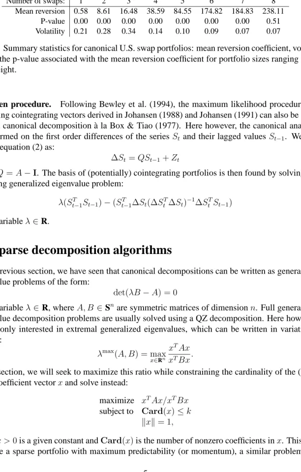
(7) whereStˆ is the least squares estimate computed above. Figure 1 gives an example of a Box & Tiao (1977) decomposition on U.S. swap rates and shows eight portfolios of swap rates with maturities ranging from one to thirty years, ranked according to predictability. Table 1 shows mean reversion coefficient, volatility and the p-value associated with the mean reversion coefficient. We see that all mean reversion coefficients are significant at the 99% level except for the last portfolio. For this highly mean reverting portfolio, a mean reversion coefficient of 238 implies a half-life of about one day, which explains the lack of significance on daily data.

Bewley et al. (1994) show that the canonical decomposition above and the maximum likelihood decomposition in Johansen (1988) can both be formulated in this manner. We very briefly recall their result below.

Number of swaps: 1 2 3 4 5 6 7 8 Mean reversion 0.58 8.61 16.48 38.59 84.55 174.82 184.83 238.11

P-value 0.00 0.00 0.00 0.00 0.00 0.00 0.00 0.51 Volatility 0.21 0.28 0.34 0.14 0.10 0.09 0.07 0.07

Table 1: Summary statistics for canonical U.S. swap portfolios: mean reversion coefficient, volatil-ity and the p-value associated with the mean reversion coefficient for portfolio sizes ranging from one to eight.

Johansen procedure. Following Bewley et al. (1994), the maximum likelihood procedure for estimating cointegrating vectors derived in Johansen (1988) and Johansen (1991) can also be writ-ten as a canonical decomposition `a la Box & Tiao (1977). Here however, the canonical analysis is performed on the first order differences of the series Stand their lagged values St−1. We can

rewrite equation (2) as:

∆St=QSt−1+Zt

whereQ=A−I_{. The basis of (potentially) cointegrating portfolios is then found by solving the}

following generalized eigenvalue problem:

λ(S_tT₋₁St−1)−(StT−1∆St(∆StT∆St)−1∆StTSt−1) (8)

in the variableλ∈R.

3

Sparse decomposition algorithms

In the previous section, we have seen that canonical decompositions can be written as generalized eigenvalue problems of the form:

det(λB₋A) = 0 (9)

in the variableλ ∈ R, whereA, B ∈Snare symmetric matrices of dimensionn. Full generalized eigenvalue decomposition problems are usually solved using a QZ decomposition. Here however, we are only interested in extremal generalized eigenvalues, which can be written in variational form as:

λmax(A, B) = max

x∈Rn

xT_Ax xT_Bx.

In this section, we will seek to maximize this ratio while constraining the cardinality of the (port-folio) coefficient vectorxand solve instead:

maximize xT_Ax/xT_Bx

subject to Card_(x)≤k

kx_k= 1,

(10)

wherek >0is a given constant andCard_{(x)is the number of nonzero coefficients inx. This will}

20 40 60 80 100 −1.2 −1.15 −1.1 −1.05 −1 −0.95 k=1 λ=−1 20 40 60 80 100 1.05 1.1 1.15 1.2 1.25 k=2 λ=16 20 40 60 80 100 −0.58 −0.57 −0.56 −0.55 −0.54 k=3 λ=62 20 40 60 80 100 0.99 1 1.01 1.02 1.03 k=4 λ=82 20 40 60 80 100 −0.98 −0.97 −0.96 −0.95 k=5 λ=117 20 40 60 80 100 0.2 0.205 0.21 0.215 k=6 λ=225 20 40 60 80 100 −0.03 −0.025 −0.02 −0.015 −0.01 k=7 λ=197 20 40 60 80 100 −0.06 −0.055 −0.05 −0.045 k=8 λ=252

Figure 1: Box-Tiao decomposition on 100 days of U.S. swap rate data (in percent). The eight canonical portfolios of swap rates with maturities ranging from one to thirty years are ranked in decreasing order of predictability. The mean reversion coefficientλis listed below each plot.

be formed to minimize it (and obtain a sparse portfolio with maximum mean reversion). This is a hard combinatorial problem, in fact, Natarajan (1995) shows that sparse generalized eigenvalue problems are equivalent to subset selection, which is NP-hard. We can’t expect to get optimal solutions and we discuss below two efficient techniques to get good approximate solutions.

3.1

Greedy search

Let us callIkthe support of the solution vectorxgivenk >0in problem (10): Ik =_{i_∈[1, n] : xi ₆= 0_},

by construction _|Ik| ≤ k. We can build approximate solutions to (10) recursively in k. When

k = 1, we simply findI1as:

I1 = argmax

i∈[1,n]

Aii/Bii.

Suppose now that we have a good approximate solution with support setIkgiven by:

xk = argmax {x∈Rn :xI c k=0} xT_Ax xT_Bx, whereIc

k is the complement of the setIk. This can be solved as a generalized eigenvalue problem

of sizek. We seek to add one variable with indexik+1 to the setIk to produce the largest increase in predictability by scanning each of the remaining indices inIc

k. The indexik+1 is then given by: ik+1 = argmax i∈Ic k max {x∈Rn:xJi=0} xT_Ax xT_Bx, whereJi =I c k\ {i},

which amounts to solving(n₋k)generalized eigenvalue problems of sizek+ 1. We then define:

Ik+1 =Ik∪ {ik+1},

and repeat the procedure untilk = n. Naturally, the optimal solutions of problem (10) might not have increasing support setsIk _⊂ Ik+1, hence the solutions found by this recursive algorithm are potentially far from optimal. However, the cost of this method is relatively low: with each iteration costingO(k2_{(n−k)), the complexity of computing solutions for all target cardinalitieskisO(n}4_).

This recursive procedure can also be repeated forward and backward to improve the quality of the solution.

3.2

Semidefinite relaxation

An alternative to greedy search which has proved very efficient on sparse maximum eigenvalue problems is to derive a convex relaxation of problem (10). In this section, we extend the techniques

of d’Aspremont, El Ghaoui, Jordan & Lanckriet (2007) to formulate a semidefinite relaxation for sparse generalized eigenvalue problems in (10):

maximize xT_Ax/xT_Bx

subject to Card_(x)≤k

kx_k= 1,

with variable x ∈ Rn. As in d’Aspremont et al. (2007), we can form an equivalent program in terms of the matrixX =xxT _∈S

n:

maximize Tr_(AX)/Tr_(BX)

subject to Card_(X)≤k2 Tr_{(X) = 1}

X 0, Rank_{(X) = 1,}

in the variableX _∈ Sn. This program is equivalent to the first one: indeed, ifX is a solution to

the above problem, then X 0and Rank_{(X) = 1 mean that we must have X = xx}T_{, while} Tr_{(X) = 1 implies thatkxk = 1. Finally, if X = xx}T _then Card_{(X) ≤ k}2 _{is equivalent to} Card_(x)≤k.

Now, because for any vectoru ∈ Rn, Card_{(u) = qimplieskuk1 ≤} √_{qkuk2, we can replace}

the nonconvex constraintCard_{(X) ≤ k}2 _{by a weaker but convex constraint}1T_|X|1 _{≤ k, using}

the fact that _kXkF =

√

xT_{x = 1 when X = xx}T _{and Tr(X) = 1. We then drop the rank}

constraint to get the following relaxation of (10):

maximize Tr_(AX)/Tr_(BX)

subject to 1T_|X|1_≤k Tr_{(X) = 1}

X 0,

(11)

which is a quasi-convex program in the variableX ∈Sn. After the following change of variables: Y = X

Tr_(BX), z =

1

Tr_(BX),

and rewrite (11) as:

maximize Tr_(AY) subject to 1T_|Y|1_{−kz ≤0} Tr_{(Y)−z = 0} Tr_{(BY) = 1} Y 0, (12)

which is a semidefinite program (SDP) in the variablesY _∈Snandz ∈R+and can be solved using

standard SDP solvers such as SEDUMI by Sturm (1999) and SDPT3 by Toh, Todd & Tutuncu (1999). The optimal value of problem (12) will be an upper bound on the optimal value of the original problem (10). If the solution matrixY has rank one, then the relaxation is tight and both optimal values are equal. When Rank_{(Y) > 1at the optimum in (12), we get an approximate}

solution to (10) using the rescaled leading eigenvector of the optimal solution matrix Y in (12). The computational complexity of this relaxation is significantly higher than that of the greedy search algorithm in_§3.1. On the other hand, because it is not restricted to increasing sequences of sparse portfolios, the performance of the solutions produced is often higher too. Furthermore, the dual objective value produces an upper bound on suboptimality. Numerical comparisons of both techniques are detailed in Section 5.

4

Parameter estimation

The canonical decomposition procedures detailed in Section 2 all rely on simple estimates of both the covariance matrixΓin (5) and the parameter matrixAin the vector autoregressive model (6). Of course, both estimates suffer from well-known stability issues and a classic remedy is to pe-nalize the covariance estimation using, for example, a multiple of the norm ofΓ. In this section, we would like to argue that using an ℓ1 penalty term to stabilize the estimation, in a procedure known as covariance selection, simultaneously stabilizes the estimate and helps isolate key id-iosyncratic dependencies in the data. In particular, covariance selection clusters the input data in several smaller groups of highly dependent variables among which we can then search for mean reverting (or momentum) portfolios. Covariance selection can then be viewed as a preprocessing step for the sparse canonical decomposition techniques detailed in Section 3. Similarly, penalized regression techniques such as the LASSO by Tibshirani (1996) can be used to produce stable, structured estimates of the matrix parameterAin the VAR model (2).

4.1

Covariance selection

Here, we first seek to estimate the covariance matrixΓby maximum likelihood. Following Demp-ster (1972), we penalize the maximum-likelihood estimation to set a certain number of coefficients in the inverse covariance matrix to zero, in a procedure known as covariance selection. Zeroes in the inverse covariance matrix correspond to conditionally independent variables in the model and this approach can be used to simultaneously obtain a robust estimate of the covariance matrix while, perhaps more importantly, discovering structure in the underlying graphical model (see Lau-ritzen (1996) for a complete treatment). This tradeoff between log-likelihood of the solution and number of zeroes in its inverse (i.e. model structure) can be formalized in the following problem:

max

X log detX−

Tr_(ΣX)−ρCard_{(X) (13)}

in the variableX ∈Sn, whereΣ∈Snis the sample covariance matrix,Card(X)is the cardinality

ofX, i.e. the number of nonzero coefficients inXandρ >0is a parameter controlling the trade-off between likelihood and structure.

Solving the penalized maximum likelihood estimation problem in (13) both improves the sta-bility of this estimation procedure by implicitly reducing the number of parameters and directly highlights structure in the underlying model. Unfortunately, the cardinality penalty makes this problem very hard to solve numerically. One solution developed in d’Aspremont, Banerjee &

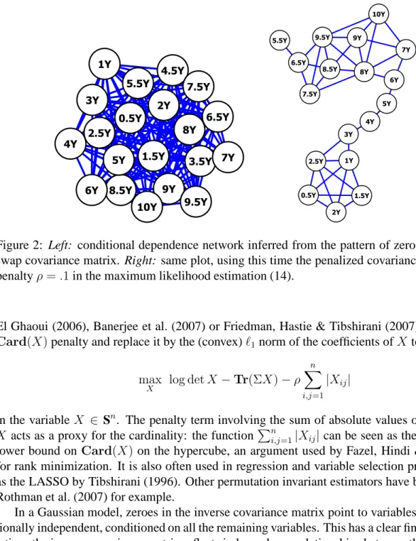
Figure 2: Left: conditional dependence network inferred from the pattern of zeros in the inverse swap covariance matrix. Right: same plot, using this time the penalized covariance estimate with penaltyρ=.1in the maximum likelihood estimation (14).

El Ghaoui (2006), Banerjee et al. (2007) or Friedman, Hastie & Tibshirani (2007) is to relax the

Card_{(X)penalty and replace it by the (convex)ℓ1 norm of the coefficients ofX to solve:}

max X log detX− Tr_(ΣX)−ρ n X i,j=1 |Xij_| (14)

in the variable X _∈ Sn. The penalty term involving the sum of absolute values of the entries of

X acts as a proxy for the cardinality: the functionPn

i,j=1|Xij|can be seen as the largest convex

lower bound onCard_{(X) on the hypercube, an argument used by Fazel, Hindi & Boyd (2001)}

for rank minimization. It is also often used in regression and variable selection procedures, such as the LASSO by Tibshirani (1996). Other permutation invariant estimators have been detailed in Rothman et al. (2007) for example.

In a Gaussian model, zeroes in the inverse covariance matrix point to variables that are condi-tionally independent, conditioned on all the remaining variables. This has a clear financial interpre-tation: the inverse covariance matrix reflects independence relationships between the idiosyncratic components of asset price dynamics. In Figure 2, we plot the resulting network of dependence, or graphical model for U.S. swap rates. In this graph, variables (nodes) are joined by a link if and only if they are conditionally dependent. We plot the graphical model inferred from the pattern of zeros in the inverse sample swap covariance matrix (left) and the same graph, using this time the penalized covariance estimate in (14) with penalty parameterρ=.1(right). The graph layout was done using Cytoscape. Notice that in the penalized estimate, rates are clustered by maturity and the graph clearly reveals that swap rates are moving as a curve.

4.2

Estimating structured VAR models

In this section, using similar techniques, we show how to recover a sparse vector autoregressive model from multivariate data.

Endogenous dependence models. Here, we assume that the conditional dependence structure of the assetsStis purely endogenous, i.e. that the noise terms in the vector autoregressive model (2) are i.i.d. with:

St =St−1A+Zt,

whereZt ∼ N(0, σI_{)for someσ >0. In this case, we must have:}

Γ =ATΓA+σI

sinceAT ⊗Ahas no unit eigenvalue (by stationarity), this means that:

Γ/σ = (I_−AT _⊗AT₎−1I

whereA_⊗B is the Kronecker product ofAandB, which implies:

ATA=I_−σΓ−1_.

We can always chooseσsmall enough so thatI_−σΓ−1 _{0. This means that we can directly getA}

as a matrix square root of(I_−σΓ−1_{). Furthermore, if we pickAto be the Cholesky decomposition}

of(I_−σΓ−1_{), and if the graph ofΓis chordal (i.e. has no cycles of length greater than three) then}

there is a permutation of the variablesP such that the Cholesky decomposition ofPΓPT_{, and the}

upper triangle of PΓPT have the same pattern of zeroes (see Wermuth (1980) for example). In Figure 4, we plot two dependence networks, one chordal (on the left), one not (on the right). In this case, the structure (pattern of zeroes) ofAin the VAR model (6) can be directly inferred from that of the penalized covariance estimate.

Gilbert (1994, _§2.4) also shows that if A satisfiesAT_{A = I−σΓ}−1 _{then, barring numerical}

cancellations inAT_{A, the graph ofΓ}−1_{is the intersection graph ofAso:}

(Γ−1)ij = 0 =⇒ AkiAkj = 0, for allk = 1, . . . , n.

This means in particular that when the graph ofΓis disconnected, then the graph ofAmust also be disconnected along the same clusters of variables, i.e. A andΓ have identical block-diagonal structure. In_§4.3, we will use this fact to show that when the graph ofΓis disconnected, optimally mean reverting portfolios must be formed exclusively of assets within a single cluster of this graph.

Exogenous dependence models. In the general case where the noise terms are correlated, with

Zt ∼ N(0,Σ)for a certain noise covarianceΣ, and the dependence structure is partly exogenous, we need to estimate the parameter matrixAdirectly from the data. In Section 2, we estimated the matrixAin the vector autoregressive model (2) by regressingStonSt−1:

ˆ

A= S_tT₋₁St−1 −1

Figure 3: Left: a chordal graphical model: no cycles of length greater than three. Right: a non-chordal graphical model.

Here too, we can modify this estimation procedure in order to get a sparse model matrix A. Our aim is again to both stabilize the estimation and highlight key dependence relationships between

Stand St−1. We replace the simple least-squares estimate above by a penalized one. We get the

columns ofAby solving:

ai = argmin

x k

Sit−St−1xk2+γkxk1 (15)

in the variablex_∈Rn, where the parameterλ >0controls sparsity. This is known as the LASSO (see Tibshirani (1996)) and produces sparse least squares estimates.

4.3

Canonical decomposition with penalized estimation

We showed that covariance selection highlights networks of dependence among assets, and that pe-nalized regression could be used to estimate sparse model matricesA. We now show under which conditions these results can be combined to extract information on the support of the canonical portfolios produced by the decompositions in Section 2 from the graph structure of the covariance matrixΓand of the model matrixA. Because both covariance selection and the lasso are substan-tially cheaper numerically than the sparse decomposition techniques in Section 3, our goal here is to use these penalized estimation techniques as preprocessing tools to narrow down the range of assets over which we look for mean reversion.

In Section 2, we saw that the Box & Tiao (1977) decomposition for example, could be formed by solving the following generalized eigenvalue problem:

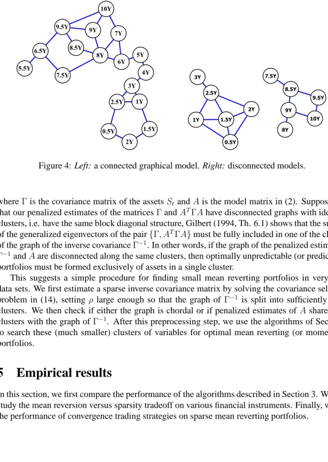
Figure 4: Left: a connected graphical model. Right: disconnected models.

whereΓis the covariance matrix of the assetsStand Ais the model matrix in (2). Suppose now that our penalized estimates of the matricesΓandAT_{ΓAhave disconnected graphs with identical}

clusters, i.e. have the same block diagonal structure, Gilbert (1994, Th. 6.1) shows that the support of the generalized eigenvectors of the pair_{Γ, AT_{ΓA}must be fully included in one of the clusters}

of the graph of the inverse covarianceΓ−1_{. In other words, if the graph of the penalized estimate of}

Γ−1_{andAare disconnected along the same clusters, then optimally unpredictable (or predictable)}

portfolios must be formed exclusively of assets in a single cluster.

This suggests a simple procedure for finding small mean reverting portfolios in very large data sets. We first estimate a sparse inverse covariance matrix by solving the covariance selection problem in (14), setting ρ large enough so that the graph of Γ−1 _{is split into sufficiently small}

clusters. We then check if either the graph is chordal or if penalized estimates of A share some clusters with the graph of Γ−1_{. After this preprocessing step, we use the algorithms of Section 3}

to search these (much smaller) clusters of variables for optimal mean reverting (or momentum) portfolios.

5

Empirical results

In this section, we first compare the performance of the algorithms described in Section 3. We then study the mean reversion versus sparsity tradeoff on various financial instruments. Finally, we test the performance of convergence trading strategies on sparse mean reverting portfolios.

5.1

Numerical performance

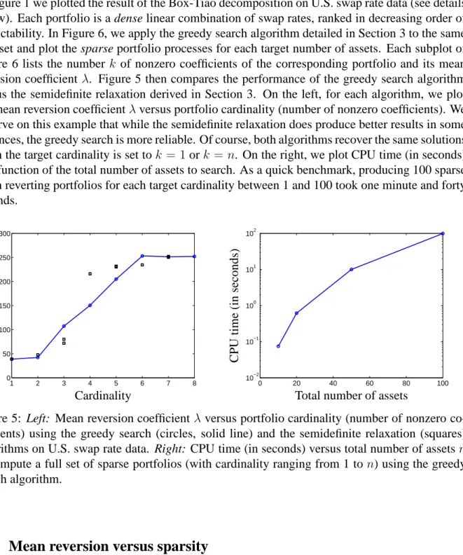
In Figure 1 we plotted the result of the Box-Tiao decomposition on U.S. swap rate data (see details below). Each portfolio is a dense linear combination of swap rates, ranked in decreasing order of predictability. In Figure 6, we apply the greedy search algorithm detailed in Section 3 to the same data set and plot the sparse portfolio processes for each target number of assets. Each subplot of Figure 6 lists the number k of nonzero coefficients of the corresponding portfolio and its mean reversion coefficient λ. Figure 5 then compares the performance of the greedy search algorithm versus the semidefinite relaxation derived in Section 3. On the left, for each algorithm, we plot the mean reversion coefficientλversus portfolio cardinality (number of nonzero coefficients). We observe on this example that while the semidefinite relaxation does produce better results in some instances, the greedy search is more reliable. Of course, both algorithms recover the same solutions when the target cardinality is set tok = 1ork = n. On the right, we plot CPU time (in seconds) as a function of the total number of assets to search. As a quick benchmark, producing 100 sparse mean reverting portfolios for each target cardinality between 1 and 100 took one minute and forty seconds. 1 2 3 4 5 6 7 8 0 50 100 150 200 250 300 Cardinality M ea n R ev er si o n 0 20 40 60 80 100 10−2 10−1 100 101 102

Total number of assets

C P U ti m e (i n se co n d s)

Figure 5: Left: Mean reversion coefficient λ versus portfolio cardinality (number of nonzero co-efficients) using the greedy search (circles, solid line) and the semidefinite relaxation (squares) algorithms on U.S. swap rate data. Right: CPU time (in seconds) versus total number of assetsn

to compute a full set of sparse portfolios (with cardinality ranging from 1 ton) using the greedy search algorithm.

5.2

Mean reversion versus sparsity

In this section, we study the mean reversion versus sparsity tradeoff on several data sets. We also test the persistence of this mean reversion out of sample.

20 40 60 80 100 6 6.2 6.4 6.6 6.8 k=1 λ=−0 20 40 60 80 100 1.35 1.4 1.45 k=2 λ=35 20 40 60 80 100 0.35 0.36 0.37 k=3 λ=128 20 40 60 80 100 0.055 0.06 0.065 0.07 0.075 0.08 k=4 λ=178 20 40 60 80 100 −0.165 −0.16 −0.155 −0.15 −0.145 k=5 λ=213 20 40 60 80 100 −0.04 −0.035 −0.03 −0.025 k=6 λ=247 20 40 60 80 100 −0.19 −0.185 −0.18 −0.175 k=7 λ=252 20 40 60 80 100 −0.06 −0.055 −0.05 −0.045 k=8 λ=252

Figure 6: Sparse canonical decomposition on 100 days of U.S. swap rate data (in percent). The number of nonzero coefficients in each portfolio vector is listed ask on top of each subplot, while the mean reversion coefficientλis listed below each one.

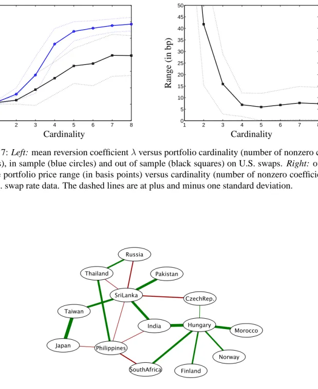
Swap rates. In Figure 7 we compare in and out of sample estimates of the mean reversion versus cardinality tradeoff. We study U.S. swap rate data for maturities 1Y, 2Y, 3Y, 4Y, 5Y, 7Y, 10Y and 30Y from 1998 until 2005. We first use the greedy algorithm of Section 3 to compute optimally mean reverting portfolios of increasing cardinality for time windows of 200 days and repeat the procedure every 50 days. We plot average mean reversion versus cardinality in Figure 7 on the left. We then repeat the procedure, this time computing the (out of sample) mean reversion in the 200 days time window immediately following our sample and also plot average mean reversion versus cardinality. In Figure 7 on the right, we plot the out of sample portfolio price range (spread between min. and max. in basis points) versus cardinality (number of nonzero coefficients) on the same U.S. swap rate data. Table 2 shows the portfolio composition for each target cardinality.

1 2 3 4 5 6 7 8 1Y 0 0 0 -0.041 -0.037 0.036 -0.013 0.001 2Y 0 0 0 0 0 0 -0.102 0.117 3Y 0 0 -0.288 0.433 0.419 -0.437 0.547 -0.495 4Y 0 -0.714 0.806 -0.803 -0.802 0.809 -0.767 0.702 5Y 1.000 0.700 -0.517 0.408 0.424 -0.389 0.317 -0.427 7Y 0 0 0 0 0 0 0 0.219 10Y 0 0 0 0 0 -0.031 0.025 -0.130 30Y 0 0 0 0 -0.007 0.016 -0.008 0.014

Table 2: Composition of optimal swap portfolios for various target cardinalities.

Foreign exchange rates. We study the following U.S. dollar exchange rates: Argentina, Aus-tralia, Brazil, Canada, Chile, China, Colombia, Czech Republic, Egypt, Eurozone, Finland, Hong Kong, Hungary, India, Indonesia, Israel, Japan, Jordan, Kuwait, Latvia, Lithuania, Malaysia, Mex-ico, Morocco, New Zealand, Norway, Pakistan, Papua NG, Peru, Philippines, Poland, Romania, Russia, Saudi Arabia, Singapore, South Africa, South Korea, Sri Lanka, Switzerland, Taiwan, Thailand, Turkey, United Kingdom, Venezuela, from April 2002 until April 2007. Note that ex-change rates are quoted with four digits of accuracy (pip size), with bid-ask spreads around0.0005

for key rates.

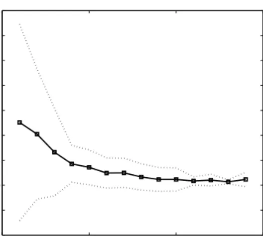
After forming the sample covariance matrixΣof these rates, we solve the covariance selection problem in (14). This penalized maximum likelihood estimation problem isolates a cluster of 14 rates and we plot the corresponding graph of conditional covariances in Figure 8. For these 14 rates, we then study the impact of penalized estimation of the matricesΓandAon out of sample mean reversion. In Figure 9, we plot out of sample mean reversion coefficientλversus portfolio cardinality, on 14 rates selected by covariance selection. The sparse canonical decomposition was performed on both unpenalized estimates and penalized ones. The covariance matrix was estimated by solving the covariance selection problem (14) withρ = 0.01and the matrixAin (2) was estimated by solving problem (15) with the penaltyγ set to zero out 20% of the regression coefficients.

We notice in Figure 9 that penalization has a double impact. First, the fact that sparse portfolios have a higher out of sample mean reversion than dense ones means that penalizing for sparsity helps prediction. Second, penalized estimates ofΓandAalso produce higher out of sample mean reversion than unpenalized ones. In Figure 9 on the right, we plot portfolio price range versus cardinality and notice that here too sparse portfolios have a significantly broader range of variation than dense ones.

5.3

Convergence trading

Here, we measure the performance of the convergence trading strategies detailed in the appendix. In Figure 10 we plot average out of sample sharpe ratio versus portfolio cardinality on a 50 days (out of sample) time window immediately following the 100 days over which we estimate the process parameters. Somewhat predictably in the very liquid U.S. swap markets, we notice that while out of sample Sharpe ratios look very promising in frictionless markets, even minuscule transaction costs (a bid-ask spread of 1bp) are sufficient to completely neutralize these market inefficiencies.

6

Conclusion

We have derived two simple algorithms for extracting sparse (i.e. small) mean reverting portfo-lios from multivariate time series by solving a penalized version of the canonical decomposition technique in Box & Tiao (1977). Empirical results suggest that these small portfolios present a double advantage over their original dense counterparts: sparsity means lower transaction costs and better interpretability, it also improved out-of-sample predictability in the markets studied in Section 5. Several important issues remain open at this point. First, it would be important to show consistency of the variable selection procedure: assuming we know a priori that only a few vari-ables have economic significance (i.e. should appear in the optimal portfolio), can we prove that the sparse canonical decomposition will recover them? Very recent consistency results by Amini & Wainwright (2008) on the sparse principal component analysis relaxation in d’Aspremont et al. (2007) seem to suggest that this is likely, at least for simple models. Second, while the dual of the semidefinite relaxation in (11) provides a bound on suboptimality, we currently have no procedure for deriving simple bounds of this type for the greedy algorithm in Section 3.1.

Acknowledgements

The author would like to thank Marco Cuturi, Guillaume Boulanger and conference participants at the third Cambridge-Princeton conference and the INFORMS 2007 conference in Seattle for helpful comments and discussions. The author would also like to acknowledge support from NSF grant DMS-0625352, ONR grant number N00014-07-1-0150, a Peek junior faculty fellowship and a gift from Google, Inc.

Appendix

In the previous sections, we showed how to extract small mean reverting (or momentum) portfolios from multivariate asset time series. In this section we assume that we have identified such a mean reverting portfolio and model its dynamics given by:

dPt=λ( ¯P −Pt)dt+σdZt, (16) In this section, we detail how to optimally trade these portfolios under various assumptions re-garding market friction and risk-management constraints. We begin by quickly recalling results on estimating the Ornstein-Uhlenbeck dynamics in (16).

Estimating Ornstein-Uhlenbeck processes

By explicitly integrating the processPtin (16) over a time increment∆twe get: Pt= ¯P +e−λ∆t(Pt−∆t−P¯) +σ

Z t

t−∆t

eλ(s−t)dZs, (17)

which means that we can estimateλandσby simply regressingPtonPt−1 and a constant. With Z t t−∆t eλ(s−t)dZs _∼ r 1−e−2λ∆t 2λ N(0,1),

we get the following estimators for the parameters ofPt:

ˆ µ = 1 N N X i=0 Pt ˆ λ = − 1 ∆t log PN i=1(Pt−µˆ)(Pt−1−µˆ) PN i=1(Pt−µˆ)(Pt−µˆ) ! ˆ σ = v u u t 2λ (1₋e−2λ∆t_)(N−2) N X i=1 ((Pt−µˆ)−e−λ∆t_(Pt−µˆ))2

where∆t is the time interval between timestandt₋1. The expression in (17) also allows us to compute the half-life of a market shock onPtas:

τ = log 2

λ , (18)

Utility maximization in frictionless markets

Suppose now that an agent invests in an assetPtand in a riskless bondBtfollowing:

dBt=rBtdt,

the wealthWtof this agent will follow:

dWt=NtdPt+ (Wt₋NtPt)rdt.

IfPtfollows a mean reverting process given by (16), this is also:

dWt = (r(Wt−NtPt) +λ( ¯P −Pt)Nt)dt+NtσdZt.

If we write the value function:

V(Wt, Pt, t) = max

Nt

E_te−β(T−t)_U(Wt),

the H.J.B. equation for this problem can be written:

βV = max Nt ∂V ∂Pλ( ¯Pt−Pt) + ∂V ∂W(r(Wt−NtPt) +λ( ¯P −Pt)Nt) + ∂V ∂t +1 2 ∂2_V ∂P2σ 2₊ 1 2 ∂2_V ∂P ∂WNtσ 2₊ 1 2 ∂2_V ∂W2N 2 tσ2

Maximizing inNtyields the following expression for the number of shares in the optimal portfolio: Nt=

∂V /∂W

∂2_{V /∂W}2_σ2(λ( ¯P −Pt)−rPt)−

∂2_{V /∂P ∂W}

∂2_{V /∂W}2 (19)

Jurek & Yang (2006) solve this equation explicitly for U(x) = logx andU(x) = x1−γ_/(1−γ)

and we recover in particular the classic expression:

Nt= λ( ¯P −Pt)−rPt σ2 Wt,

in the log-utility case.

Leverage constraints

Suppose now that the portfolio is subject to fund withdrawals so that the total wealth evolves according to:

dW =dΠ +dF

wheredΠ =NtdPt+ (Wt−NtPt)rdtanddF represents fund flows, with: dF =f dΠ +σfdZt(2)

whereZt(2)is a Brownian motion (independent ofZt). Jurek & Yang (2006) show that the optimal

portfolio allocation can also be computed explicitly in the presence of fund flows, with:

Nt= λ( ¯P ₋Pt)₋rPt σ2 1 (1 +f)Wt =LtWt,

in the log-utility case. Note that the constantf can also be interpreted in terms of leverage limits. In steady state, we have:

Pt∼ N ¯ P ,σ 2 2λ

which means that the leverage Lt itself is normally distributed. If we assume for simplicity that

¯

P = 0, given the fund flow parameterf, the leverage will remain below the levelM given by:

M = α(λ+r)

(1 +f)σ√2λ (20)

with confidence levelN(α), whereN(x)is the Gaussian CDF. The bound on leverageM can thus be seen as an alternate way of identifying or specifying the fund flow constantfin order to manage capital outflow risks.

References

Alexander, C. (1999), ‘Optimal hedging using cointegration’, Philosophical Transactions: Mathematical, Physical and Engineering Sciences 357(1758), 2039–2058.

Amini, A. & Wainwright, M. (2008), ‘High dimensional analysis of semidefinite relaxations for sparse principal component analysis’, Tech report, Statistics Dept., U.C. Berkeley .

Banerjee, O., Ghaoui, L. E. & d’Aspremont, A. (2007), ‘Model selection through sparse maximum likeli-hood estimation’, ICML06. To appear in Journal of Machine Learning Research.

Bewley, R., Orden, D., Yang, M. & Fisher, L. (1994), ‘Comparison of Box-Tiao and Johansen Canonical Estimators of Cointegrating Vectors in VEC (1) Models’, Journal of Econometrics 64, 3–27.

Box, G. E. & Tiao, G. C. (1977), ‘A canonical analysis of multiple time series’, Biometrika 64(2), 355. Campbell, J. & Viceira, L. (1999), ‘Consumption and Portfolio Decisions When Expected Returns Are Time

Varying’, The Quarterly Journal of Economics 114(2), 433–495.

Cand`es, E. J. & Tao, T. (2005), ‘Decoding by linear programming’, Information Theory, IEEE Transactions on 51(12), 4203–4215.

Candes, E. & Tao, T. (2007), ‘The Dantzig selector: statistical estimation when$ p$ is much larger than$ n$’, To appear in Annals of Statistics .

Chen, S., Donoho, D. & Saunders, M. (2001), ‘Atomic decomposition by basis pursuit.’, SIAM Review

d’Aspremont, A., Banerjee, O. & El Ghaoui, L. (2006), ‘First-order methods for sparse covariance selec-tion’, To appear in SIAM Journal on Matrix Analysis and Applications .

d’Aspremont, A., El Ghaoui, L., Jordan, M. & Lanckriet, G. R. G. (2007), ‘A direct formulation for sparse PCA using semidefinite programming’, SIAM Review 49(3), 434–448.

Dempster, A. (1972), ‘Covariance selection’, Biometrics 28, 157–175.

Dickey, D. & Fuller, W. (1979), ‘Distribution of the Estimators for Autoregressive Time Series With a Unit Root’, Journal of the American Statistical Association 74(366), 427–431.

Donoho, D. L. & Tanner, J. (2005), ‘Sparse nonnegative solutions of underdetermined linear equations by linear programming’, Proc. of the National Academy of Sciences 102(27), 9446–9451.

Engle, R. & Granger, C. (1987), ‘Cointegration and error correction: representation, estimation and testing’, Econometrica 55(2), 251–276.

Fama, E. & French, K. (1988), ‘Permanent and Temporary Components of Stock Prices’, The Journal of Political Economy 96(2), 246–273.

Fazel, M., Hindi, H. & Boyd, S. (2001), ‘A rank minimization heuristic with application to minimum order system approximation’, Proceedings American Control Conference 6, 4734–4739.

Friedman, J., Hastie, T. & Tibshirani, R. (2007), ‘Sparse inverse covariance estimation with the lasso’, Working paper .

Gatev, E., Goetzmann, W. & Rouwenhorst, K. (2006), ‘Pairs Trading: Performance of a Relative-Value Arbitrage Rule’, Review of Financial Studies 19(3), 797.

Gilbert, J. (1994), ‘Predicting Structure in Sparse Matrix Computations’, SIAM Journal on Matrix Analysis and Applications 15(1), 62–79.

Grossman, S. & Vila, J. (1992), ‘Optimal Dynamic Trading with Leverage Constraints’, The Journal of Financial and Quantitative Analysis 27(2), 151–168.

Johansen, S. (1988), ‘Statistical analysis of cointegration vectors’, Journal of Economic Dynamics and Control 12(2/3), 231–254.

Johansen, S. (1991), ‘Estimation and Hypothesis Testing of Cointegration Vectors in Gaussian Vector Au-toregressive Models’, Econometrica 59(6), 1551–1580.

Jurek, J. & Yang, H. (2006), Dynamic portfolio selection in arbitrage, Technical report, Working Paper, Harvard Business School.

Kim, T. & Omberg, E. (1996), ‘Dynamic Nonmyopic Portfolio Behavior’, The Review of Financial Studies

9(1), 141–161.

Lauritzen, S. (1996), ‘Graphical Models’.

Liu, J. & Longstaff, F. (2004), ‘Losing Money on Arbitrage: Optimal Dynamic Portfolio Choice in Markets with Arbitrage Opportunities’, Review of Financial Studies 17(3).

Meinshausen, N. & Yu, B. (2007), Lasso-type recovery of sparse representations for highdimensional data, Technical report, To appear in Annals of Statistics.

Natarajan, B. K. (1995), ‘Sparse approximate solutions to linear systems’, SIAM J. Comput. 24(2), 227–234. Poterba, J. M. & Summers, L. H. (1988), ‘Mean reversion in stock prices: Evidence and implications’,

Journal of Financial Economics 22(1), 27–59.

Rothman, A., Bickel, P., Levina, E. & Zhu, J. (2007), ‘Sparse permutation invariant covariance estimation’, Technical report 467, Dept. of Statistics, Univ. of Michigan .

Sturm, J. (1999), ‘Using SEDUMI 1.0x, a MATLAB toolbox for optimization over symmetric cones’, Op-timization Methods and Software 11, 625–653.

Tibshirani, R. (1996), ‘Regression shrinkage and selection via the LASSO’, Journal of the Royal statistical society, series B 58(1), 267–288.

Toh, K. C., Todd, M. J. & Tutuncu, R. H. (1999), ‘SDPT3 – a MATLAB software package for semidefinite programming’, Optimization Methods and Software 11, 545–581.

Wachter, J. (2002), ‘Portfolio and Consumption Decisions under Mean-Reverting Returns: An Exact Solu-tion for Complete Markets’, The Journal of Financial and Quantitative Analysis 37(1), 63–91. Wermuth, N. (1980), ‘Linear Recursive Equations, Covariance Selection, and Path Analysis’, Journal of the

American Statistical Association 75(372), 963–972.

Xiong, W. (2001), ‘Convergence trading with wealth effects: an amplification mechanism in financial mar-kets’, Journal of Financial Economics 62(2), 247–292.

Yuan, M. & Lin, Y. (2007), ‘Model selection and estimation in the Gaussian graphical model’, Biometrika

1 2 3 4 5 6 7 8 −50 0 50 100 150 200 250 300 Cardinality M ea n R ev er si o n 1 2 3 4 5 6 7 8 0 5 10 15 20 25 30 35 40 45 50 Cardinality R an g e (i n b p )

Figure 7: Left: mean reversion coefficientλversus portfolio cardinality (number of nonzero coef-ficients), in sample (blue circles) and out of sample (black squares) on U.S. swaps. Right: out of sample portfolio price range (in basis points) versus cardinality (number of nonzero coefficients) on U.S. swap rate data. The dashed lines are at plus and minus one standard deviation.

Figure 8: Graph of conditional covariance among a cluster of U.S. dollar exchange rates. Posi-tive dependencies are plotted as green links, negaPosi-tive ones in red, while the thickness reflects the magnitude of the covariance.

0 2 4 6 8 10 12 14 −20 0 20 40 60 80 100 120 140 Cardinality M ea n R ev er si o n 0 5 10 15 −1 −0.5 0 0.5 1 1.5 2 2.5 3 3.5 Cardinality R an g e

Figure 9: Left: out of sample mean reversion coefficient versus portfolio cardinality (number of nonzero coefficients), on 14 U.S. dollar exchange rates clustered by covariance selection. The sparse canonical decomposition was performed on both unpenalized estimates (black squares) and penalized ones (blue circles). Right: out of sample portfolio price range (in percent) versus cardi-nality. The dashed lines are at plus and minus one standard deviation.

1 2 3 4 5 6 7 8 −2 0 2 4 6 8 10 Cardinality S h ar p e R at io 1 2 3 4 5 6 7 8 −3 −2 −1 0 1 2 3 Cardinality S h ar p e R at io

Figure 10: Left: average out of sample sharpe ratio versus portfolio cardinality on U.S. swaps.

Right: idem, with a bid-ask spread of 1bp. The dashed lines are at plus and minus one standard