ABSTRACT
The radiosity method models the interaction of light between dif-fuse surfaces, thereby accurately predicting global illumination effects. Due to the high computational effort to calculate the trans-fer of light between surfaces and the memory requirements for the scene description, a distributed, parallelized version of the algo-rithm is needed for scenes consisting of thousands of surfaces.
We present several load distribution schemes for such a paral-lel algorithm which includes progressive refinement and adaptive subdivision for fast solutions of high quality. The load is distrib-uted before the calculations in a static way. During the computa-tion the load is redistributed dynamically to make up for individual differences in processor loads. The dynamic load balancing scheme never generates more data packets than the original algo-rithm and avoids overloading processors through actions taken by the scheme.
CR Categories and Subject Descriptors: I.3.7 [Computer Graphics]: Three-Dimensional Graphics and Realism.
1 Introduction
Radiosity has become a popular method for image synthesis due to its ability to generate images of high realism. It was first intro-duced to computer graphics by Goral et al. [11]. Further research resulted in the progressive refinement method, which quickly pro-duces good approximations of the final solution [8]. For recent developments see [9],[20].
Common to all these methods is the representation of the sur-faces of the environment by a mesh of quadrilaterals and triangles. These “patches” are used to store the radiosity on the respective part of the surface. Other surface representations (eg. freeform sur-faces, CSG models, ...) must be approximated by triangles.
A formfactor is a value describing the “influence” of two patches onto each other. These formfactors were first calculated by the use of a hemicube [6]. A hemicube is placed around the centre of a patch and all other patches are projected onto its surfaces. The
projected area gives an estimate for the formfactor between the patches. As this estimate of the formfactors may be inexact even for simple cases [1], other methods for computing the formfactors were suggested. Sillion [18] used a single plane for the projection; Wallace [26] introduced ray-traced formfactors; Malley [14] pro-posed a stochastic method.
During the calculation of the formfactors the visibility calcula-tions account for most of the computation time of the radiosity method (e.g. 70 - 95%) and the memory requirement increases with the number of patches. These problems led to the develop-ment of parallel impledevelop-mentations of the progressive refinedevelop-ment radiosity method [2], [16], [10], [5].
This paper presents a MIMD implementation of the radiosity method suitable for massively parallel computers. In section 2 the basic parallel progressive refinement algorithm is discussed which is generalized for distributed visibility calculations in section 3. Static and dynamic load balancing schemes are introduced in sec-tion 4 and secsec-tion 5 the timings of which are thereafter compared to each other and to the original version in section 6.
1.1 Progressive Refinement
The radiosity method partitions the surfaces of the scene in small, flat patches and computes the illumination for each of those patches. The radiosity of a patch is determined by the radiosity it emits directly plus all light that is reflected. This is described by the radiosity equation
where
• n is the number of the patches. • Bi is the radiosity of the i-th patch. • Ei is the emitted radiosity of the i-th patch. •ρi is the reflectivity of the i-th patch. • Fi,j is the formfactor from patch i to patch j.
The linear equation system defined above can be solved with an iterative Gauss-Seidel solution method and converges quickly in practice. As the memory requirement for the formfactor matrix is proportional to n2 this method becomes impractical for larger n (n > 10000). Also the computational effort to compute all Fi,j becomes prohibitively large.
The progressive refinement method [8] uses a reordering of the solution process which just needs to calculate (and store) one
col-Bi Ei ρi Fi j, Bj j=0 n–1
∑
+ =Load Balancing for a Parallel Radiosity Algorithm
W. Stürzlinger
1, G. Schaufler
1and J. Volkert
1GUP, Johannes Kepler Universität Linz, AUSTRIA
1 Kepler University,Altenbergerstr.69,A-4040 Linz,Austria/Europe
umn of the matrix per iteration step. The patch with most unshot radiosity is selected as the shooter and its radiosity is distributed to all other patches in the environment by calculating form factors from the shooter to the receiving patches. While the solution con-verges an intermediate picture can be displayed after each iteration step.
1.2 Patches and Elements
If the patches are too big, the quality of the approximation of the illumination function across the objects’ surfaces will be poor. One solution is to use smaller patches which increases both memory and cpu time consumption. However, for shooting the radiosity bigger patches have been found to give sufficiently accurate results and, therefore, a two-level hierarchy of patches and elements was proposed by Cohen et al. [7]. Each patch is subdivided into ele-ments. The radiosity is computed for all elements which are used during display of the solution. The average of the element radiosi-ties is used as the patch radiosity for shooting.
1.3 Adaptive Subdivision
Adaptive subdivision [9] extends the two level hierarchy of patches and elements to a hierarchy of several levels: whenever the radiosi-ties at the corners of an element differ by more than a given thresh-old the element is subdivided into several smaller elements and only the influence of the current shooter must be recalculated for the new elements. As a result more elements are generated in areas of large illumination variations (shadow boundaries) and a better approximation of the illumination function is achieved.
2 Parallelization of the Progressive Refinement
Method
Though the progressive refinement method converges much faster than the conventional radiosity method its computational complex-ity still makes a parallel implementation desirable.
2.1 Previous Research
Parallelizations of the progressive refinement method have been proposed by Baum [2] for a multiprocessor workstation and Recker [16] for a cluster of workstations. Feda [10] and Chalmers [5] presented an implementation on a transputer network with local memory on each transputer.
Both the hemicube used by Baum and Feda and the analytical method used by Chalmers and Recker suffer from the problem that the formfactors and the visibilities are determined using the shooter as the projection centre which leads to noticeable artifacts. A better method is to calculate formfactors and visibilities directly for each receiver.
Even most recent implementations such as those by Capin et al.[3], Ng et al. [15] and Lamotte et al. [13] are not easily extended to parallel computers of several hundred processors. Capin uses one ring of processors where round trip times become prohibitively large. Ng and Lamotte use master-slave approaches where the mas-ter soon becomes the bottle neck.
In the following sections we assume that we have a number of processors with local memory and an interconnecting network.
2.2 Parallel Progressive Refinement
This paper presents an approach based on the calculation of form-factors by raycasting as described by Wallace [26]. Raycasting is used to determine the visible parts of the shooter as seen from each
receiving patch. The formfactor of these visible parts is then calcu-lated using the analytical solution to the contour integral. The visi-bility is determined by subdividing the shooter regularly into M parts and casting a ray from the receiving patch to each of these parts.
We distribute the n patches evenly among the N processors, and each processor computes the radiosity for it’s patches by computing the energy received from the shooter. The shooter is selected by a global maximum search and is broadcast by the mas-ter to all other processors.
For visibility computations we must store the complete scene geometry on each processor. Therefore, the maximum number of patches which can be handled by the algorithm is limited by the available memory on each processor. In section 3 we will show how this algorithm can be extended for larger numbers of patches.
The following steps are performed until the solution has con-verged:
• All processors send their local shooter to the master processor, i.e. the patch which has the most unshot radiosity.
• The master processor chooses the global shooter and sends this information to all processors. Note that the shooter-geometry and the associated radiosity values are distributed to all proces-sors in this step also.
• The following steps are performed on all processors in parallel: For each receiving patch we determine the visibility of the shooter by casting rays to the shooter. Each ray is inter-sected with all other patches. For the visible parts the geo-metric formfactor is calculated and the resulting contribution is added to the receiver’s radiosity.
In contrast to many previously presented algorithms, no radiosity values need to be updated on other processors. The only communi-cation overhead is generated by the selection and distribution of the shooter once for each iteration step and can be optimized using the topology of the parallel machine.
After every p-th iteration (p is user selectable) an intermediate picture can be rendered by sending all patches to a graphics work-station. This image generation is not discussed further in this paper.
3 Visibility Determination
The major shortcoming of the algorithm presented in section 2.2 is that the number of patches is limited by the available memory on each processor because the visibility of the shooter must be deter-mined locally.
3.1 Parallel Visibility Calculation
When there is not enough memory to store all patches on one pro-cessor the data transfer overhead becomes prohibitively large if patch geometries are retrieved from other processors [10], [5].
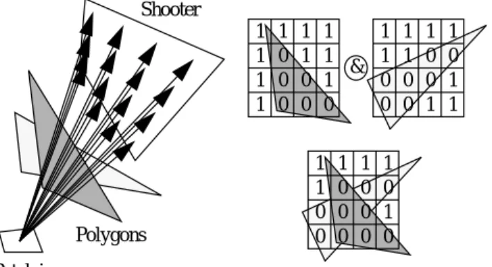
Instead of transferring patches to compute visibility, we trans-fer the sampling points with respective visibility information. Using a fixed subdivision of the shooter into M (e.g. 16 or 64) parts the visibility for each part is determined by casting a ray to the part’s centre. The ratio of all visible parts to the total number of parts gives an approximation to the visibility of the shooter from the sampling point. This visibility information for each sampling
n N
----point can be stored in a bit vector of length M (see also figure 1).
Figure 1. Parallel Visibility Computations
Once the scene patches are evenly distributed among the available processors, every processor can calculate the visibility of the shooter using its set of patches. The binary AND operation of the visibility vectors of all processors determines the visibility of the shooter with respect to the whole scene.
Stürzlinger et al. [24] proposed to arrange the processors in a ring which is used as a pipeline for packets of sampling point. Each processor generates a packet, sends it around the ring, computes the local visibility of the samples in the packet and ANDs it to the visibility vectors in the packet. When the packet returns to the pro-cessor it originated from the local visibility is ANDed and the form factors can be calculated.
3.2 Optimized Parallel Visibility Calculations
As long as the processors have enough local memory so that not all of them are needed to store the samples and the scene, more than one ring can be used in parallel. The processors are organized into several separate rings and the patch geometries are stored once in each ring. One processor holds the patches and elements it com-putes radiosities for and a set of patch geometries for visibility computations.Figure 2. Sample patch assignments for 2 rings with 3 processors In figure 2 an example patch assignment for a scene consisting of 6 patches onto 2 rings with 3 processors each is shown. The bold numbers (p1 - p6) denote patches for which radiosity is calculated and the italic numbers (g1-g6) denote patch geometries stored for visibility calculations.
The geometric formfactor and the maximum energy trans-ferred between the sampling point and the shooter gives a measure how precise visibilities need to be calculated and how many rays must be cast to the shooter.
3.3 The Global BSP-Tree
The overwhelming amount of computation carried out on all
pro-cessors is the intersection of rays with scene patches to determine the visibility of the shooter. A BSP-tree is commonly used to speed up the intersection of rays with a large number of polygons. Poly-gons are classified as lying in one or more of the subspaces defined by the BSP-tree. Only those polygons situated in subspaces pene-trated by the ray must be considered (see e.g. [25]).
Caspary et al. [4] introduced a new method of storing such a BSP-tree in the local memory of processors of a parallel computer. The upper part of the tree from the root node down to some prede-termined level of subdivision is stored on all processors. This part of the BSP-tree is referred to as the global BSP-tree. The subtrees below the global BSP-tree are each stored on one processor only. All other processors replace the subtree with a reference pointing to the processor storing the respective subtree.
Figure 3. The global BSP-tree
Note that one processor may store more than one subtree and that the global BSP-tree is not balanced (figure 3).
During setup the global BSP-tree is generated on the host com-puter and broadcast to all processors. This global BSP-tree defines a subdivision of the scene-space which is the same on all proces-sors. Now the patches are broadcasted to the processors as well and all processors in parallel filter out the patches which intersect their subspaces and insert them into their local subtree.
The global BSP-tree allows each processor to determine for any ray which processors must contribute to the intersection of the ray with all polygons in the global BSP-tree. On the ring-topology of processors introduced by Stürzlinger [24] it can be calculated in advance to which processors in the ring the packet must be sent and which can be left out. This information is added to the contents of the packet as a processor vector.
3.4 Processor Vectors
The processor vector is an array of flags in the sample packet con-taining one flag for each processor in the ring. If the flag for a pro-cessor is set, the sample packet must be sent to and processed by the corresponding processor. By the use of the global BSP-tree the processor vector can be computed by any processor, in particular by the processor generating the sample packet. Whenever a packet is sent around the ring the next processor is determined by finding the next set flag in the processor vector, thereby leaving out proces-sors which do not influence the visibility bit-vector of the samples in the packet and reducing the communication in the rings.
Two user defined limits determine the maximum number of samples in one packet and the maximum number of processors which must be visited in the ring. If one of the limits is exceeded, no more samples are added to the packet and the packet is pro-cessed by the ring.
4 Static Load Balancing
At the begin of each iteration all processors are synchronized by the selection of the shooting patch. As a result the slowest proces-sor dictates the total iteration time. Load Balancing aims at distrib-uting storage and computational demand equally among processors 1 1 1 1 1 0 1 1 1 0 0 1 1 0 0 0 1 1 1 1 1 1 0 0 0 0 0 1 0 0 1 1 & 1 1 1 1 1 0 0 0 0 0 0 1 0 0 0 0 Shooter Polygons Patch i
p1
p3
p2
g1 g2
g3 g4
g5 g6
p4
p6
p5
g1 g2
g3 g4
g5 g6
Subtree on Proc 0 Subtree on Proc 1 Subtree on Proc 1 Subtree on Proc 0 Subtree on Proc 3 Subtree on Proc 2so that the iteration time is approximately the same on all proces-sors. Static load balancing distributes the data needed during com-putation in a way so that comparable load can be expected on all processors.
4.1 Static Load Balancing of Radiosity Samples
Supposed that each radiosity element causes the same amount of computation equal load can be expected on each processor if each processor computes the same amount of element radiosities. As different patches are subdivided into different numbers of elements it is insufficient to only assign the same amount of patches to one processor. Patches with large numbers of elements must be split into smaller ones to allow an even distribution of elements among processors [23]. This necessity slightly increases the total number of patches but results in considerable gain in processing speed as equal amounts of computation are initially assigned to each proces-sor (see table 2 in section 6 for timings of this load balancing scheme applied in combination with the scheme described in the following section 4.2).When adaptive refinement is used the balance of computation will be destroyed as new elements are introduced on selected pro-cessors. It cannot be determined in advance (during setup) where such refinement will occur and, therefore, static load balancing is not suitable to compensate for the resulting imbalance. A dynamic scheme is needed which is introduced in section 5.2.
4.2 Static Load Balancing of Visibility Complexity
For each sample on an element the visibility of the shooter must be determined. The complexity of these visibility tests is primarily due to the number of polygons stored in one processors local BSP-trees. Therefore, the size of the global BSP-tree must be chosen big enough, so that approximately the same number of patches is assigned to each processor by selecting the local BSP-trees stored on it.The selection of the global BSP-tree size is subject to a mem-ory vs. distribution quality trade-off: the bigger the global BSP-tree, the lower variations in the distribution of polygons onto pro-cessors can be achieved. At the same time a bigger global BSP-tree results in more memory consumption on each processor as the glo-bal BSP-tree must be stored on each of them. The time savings attained with static load balancing of visibility complexity are summarized in table 2 in section 6 and should be compared with table 1 which lists the calculation times without static load balanc-ing.
However, the time needed to compute the visibility tests may still vary when large subtrees of the processor’s local BSP-tree can be classified as not being intersected by the ray. Such variations cannot be compensated for by static load balancing as they are not predictable at the beginning of the computation. Moreover, adap-tive refinement can introduce an arbitrary number of additional ele-ments on any processor which increases this processor’s load significantly.
5 Dynamic Load Balancing
Dynamic load balancing tries to influence individual processors iteration times by transferring work from loaded to less loaded pro-cessors in order to speed up the completion of one iteration.
5.1 Dynamic Load Balancing of Visibility Tests
As a first attempt dynamic load balancing of visibility tests was tried but did not yield satisfactory results for reasons which were not evident from the beginning. In this scheme the time needed toprocess all sample packets arriving at a processor in a ring is used as a measure for the load of the processor. After each iteration loaded processors are determined and an adequate part of their work for the next iteration is transferred to less loaded processors.
As the computational load is primarily due to visibility tests the distribution of the patches must be rearranged to perform dynamic load balancing of visibility tests. However, changing the distribution of patches among processors and rearranging the BSP-tree is a very costly operation. Moreover the load of the last itera-tion is rarely a good estimate for the load of the next iteraitera-tion as a new shooter is selected for each iteration and the spatial relations of samples and shooter change completely. The implementation of such a dynamic load balancing scheme of visibility tests did always slow down the iterations and, therefore, no timings are given in section 6.
5.2 Dynamic Load Balancing of Sample Packets
A better possibility for dynamic load balancing computation from loaded processors to processors which already finished the current iteration. In this way the load of the current iteration is used to guide the balancing of computations. Moving the computation of a sample packet from one ring to another means transferring all the visibility computations for this packet to the other ring at very little cost: all the information for these computations are already avail-able on the other ring and this ring also has the availavail-able capacity to process the packet as the processor is already idle and will not generate any further packets itself.The idea of balancing sample packets is to make use of proces-sors which have already finished generating sample packets in the current iteration and identify them as idle. An idle processors in one ring request sample packets from loaded processors in other rings, has them processed in its own ring and sends them back to the loaded processor. These steps are repeated until all processors have finished the current iteration.
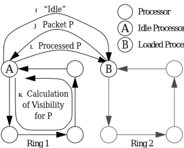
The figure below depicts the involved steps in detail: when pro-cessor A in ring 1 has finished the calculations on the last sampling package generated by it, it sends an “Idle” message to a processor B in a randomly chosen other ring but at the same position in the ring. If Processor B still has unprocessed sample packets it sends a packet P to processor A. Processor A initializes the visibility com-putations of packet P, sends it around the ring and returns it to Pro-cessor B afterwards. ProPro-cessor A repeats the random polling until all processors have finished the current iteration.
The method of random polling was chosen as the work of Kumar et al. [12] shows that this method is in general superior to all other methods considered by them in a comprehensive survey, especially when used with massively parallel computer systems.
Figure 4. Dynamic Load Distribution of Sample Packets As idle processors do not generate any packets themselves but only
Ring 1 Ring 2 Processor
A
➀“Idle” ➁ Packet P ➃ Processed P ➂Calculation of Visibility for PA
B
Idle Processor Loaded ProcessorB
introduce one packet from another ring at a time this scheme guar-antees that a ring with idle processors is not overloaded by too many packets from other rings. The amount of packets circulating in a ring is not increased by this dynamic load balancing scheme as there are never more packets in the ring than processors.
Processors which are polled for load balancing packets and are already idle themselves respond with a list of processors which they already found to be idle (including their own id) so that unnecessary random polling is minimized and only introduces moderate communication overhead. A parallel termination algo-rithm determines when the global shooter selection can initiate for the next iteration.
Table 3 in section 6 shows the time advantage of this dynamic load balancing scheme when compared to the tables before and table 4 gives timings for dynamic load balancing in combination with full static load balancing.
6 Implementation and Results
Our approach was implemented on an nCube2S with 256 proces-sors - a distributed memory computer the nodes of which are con-nected with a hypercube topology network. The performance of a single processor is approximately 3 MFLOPS.
As a basis we used the progressive radiosity program described by Stürzlinger et al. [21]. The algorithm has been improved to use a global BSP-Tree (described in section 3.3) and it includes static load balancing of radiosity samples (see section 4.1) and of visibil-ity complexvisibil-ity (see section 4.2). Moreover two dynamic load bal-ancing schemes have been implemented (section 5.1 and section 5.2) of which the latter performs very well both in combination with and without static load balancing. The tests have shown dynamic load balancing to be particularly useful with adaptive refinement as it increases the number of certain samples in a way not predictable before the begin of the calculations [17].
All times were measured using sample packets of 50 samples each. In the following tables and figures N denotes the number of processors and R denotes the length of the rings. A scene of a sim-ple living room consisting of 4738 patches with a total of 17251 elements was used. Due to the memory constraints it took at least rings of 4 processors to store the scene and at least a total of 8 pro-cessors to store all the samples. All timings are given in seconds for the average of the first four iterations of the algorithm to com-plete. Later shooting operations generally take less time as less energy is distributed. Configurations where the processors ran out of local memory are marked “out of mem”. Table 1 summarizes run-times with load balancing disabled.
Table 2 gives the run-times of the algorithm when static load
bal-ancing has been performed before the iterations are started.
The run-times for dynamic load balancing (described in section 5.2), i.e. without static load balancing are summarized in table 3.
Table 4 shows the run-times for the first iteration of the algorithm when both static and dynamic load balancing are enabled. The val-ues given in the diagonal of the table are equal to those given in table 2 as no dynamic load balancing is possible with just one ring. However, with all other configurations the combination of static and dynamic load balancing yields the best results.
Test runs with a more complex scene showed that the 4738 patch scene is too small to demonstrate the capabilities of this dynamic load balancing scheme. Moreover with adaptive subdivision of sur-faces static distribution of patches to processors are outdated by the new patches introduced by the adaptive subdivision algorithm. The dynamic load balancing scheme presented in this paper made a speed-up of 26% possible for the radiosity simulation of a scene with approximately 60000 patches and approx. 100000 (131000) elements before (after) four iterations (see table 5). As the undis-tributed energy decreases generally with each iteration the subdivi-sion criterion is met less often and the rate of element subdivisubdivi-sion
N \ R 4 8 16 32 64 128 256 4 out of mem 8 out of mem 155 16 out of mem 79 129 32 35.5 51 74 117.5 64 29.5 38.3 45.3 66.3 113.3 128 31.5 39 46.5 49 67.5 108.5 256 29.5 36 39 47 67.3 74.8 81
Table 1: No Load Balancing (N=#processors, R=#rings)
N \ R 4 8 16 32 64 128 256 4 out of mem 8 out of mem 155 16 out of mem 79.5 129 32 25 37.5 54 82.5 64 13.3 20.5 28.5 48.3 74.8 128 7 8.5 13 21.5 36.5 57 256 5 8.3 7.8 9 13.3 16.3 28.3
Table 2: Static Load Balancing (N=#processors, R=#rings)
N \ R 4 8 16 32 64 128 256 4 out of mem 8 out of mem 155 16 out of mem 73.3 129 32 32.3 39.3 65.3 117.5 64 20.5 21.5 34.3 62.8 113.3 128 15.5 14.5 20 33 56.8 108.5 256 11.5 13.3 11.3 15 28 75.5 81
Table 3: Dynamic Load Balancing (N=#processors, R=#rings)
N \ R 4 8 16 32 64 128 256 4 out of mem 8 out of mem 155 16 out of mem 73.5 129 32 22.8 34.8 50 82.5 64 12.5 19.5 25.3 44 74.8 128 6 7.8 12 21.5 36.5 57 256 4.8 7.8 7.5 8.5 12.3 16 28.3
Table 4: Static and Dynamic Load Balancing (N=#processors, R=#rings)
decreases as well.
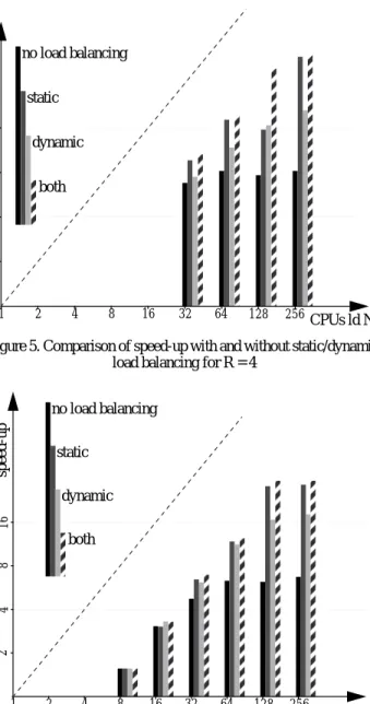
The following two diagrams allow to compare the speed-up of the different load balancing schemes for configurations with rings of 4 processors from a total of 32 to 256 processors and for 8 processors from a total of 8 to 256 processors. The speed-up was calculated in relation to an extrapolated timing using a serial version of the pro-gram running on a Sun 4/330. Considering the MFLOPS perfor-mance of both the Sun and one processor node of the parallel computer the extrapolated runtime for this serial version on a sin-gle processor node is estimated to be 242 seconds. This work-around was used because the limited memory available on one node of the nCube2S did not allow to obtain timings for a serial run.
Figure 5. Comparison of speed-up with and without static/dynamic load balancing for R = 4
Figure 6. Comparison of speed-up with and without static/dynamic load balancing for R=8
As one can see from the diagrams static load balancing yields good results in general, if it fails, however, dynamic load balancing fur-ther improves the performance even furfur-ther (cf. figure 5, 128 CPUs).
7 Conclusions
This paper reports on several major improvements over the parallel radiosity algorithm described by Stürzlinger et al. [24]. First a glo-bal BSP-Tree has been introduced as a data structure to speed up ray-patch intersections and to optimize the routing of sample pack-ets around the processor rings in conjunction with processor vec-tors.
Second, two strategies for static load balancing have been pro-posed: static load balancing of radiosity samples provides an even distribution of radiosity samples and associated computations over the processors; static load balancing of visibility complexity makes best use of local processor memory and computational capacity to solve the visibility problem which is responsible of about 70-90% of the computation in a radiosity solution.
Third, two strategies for dynamic load balancing have been implemented and the second one has been found to be particularly successful on massively parallel computers in combination with the method of adaptive refinement.
Further research will be carried out to increase the accuracy of the form factor calculations and to compare them to exact methods. Moreover, the existing meshing algorithms could be improved by using discontinuity meshing to better approximate the illumination of the scene.
References
[1] Baum, Daniel R., Holly E. Rushmeier and James M. Winget, “Improving Radiosity Solutions through the Use of Analyti-cally Determined Form-Factors”, Computer Graphics (ACM SIGGRAPH ‘89 Proceedings) 23 3 (July 1989) pp 325-334. [2] Baum, Daniel R. and James M. Winget, “Real Time Radiosity
Through Parallel Processing and Hardware Acceleration”, Computer Graphics (1990 Symposium on Interactive 3D Graphics) 24 2 (March 1990) pp 67-75.
[3] Capin, T. K., C. Aykanat and B. Özgüc, “Progressive Refine-ment Radiosity on Ring-Connected Multicomputers”, Parallel Rendering Symposium (Oct. 1993) pp 71-88.
[4] Caspary, E. and I. D. Scherson, “A self-balanced parallel ray-tracing algorithm”, Parallel Processing for Computer Vision and Display, P. M. Dew, R. A. Earnskaw, T.R. Heywood (Ed.), Addison Wesley, 1989.
[5] Chalmers, Alan G. and Derek J. Paddon, “Parallel Processing of Progressive Refinement Radiosity Methods”, Photorealistic Rendering in Computer Graphics (Proceedings of the Second Eurographics Workshop on Rendering) Springer-Verlag New York 1994 pp 149-159.
[6] Cohen, Michael and Donald P. Greenberg, “The Hemi-Cube: A Radiosity Solution for Complex Environments”, Computer Graphics (ACM SIGGRAPH ‘85 Proceedings) 19 3 (Aug. 1985) pp 31-40.
[7] Cohen, Michael, Donald P. Greenberg, Dave S. Immel, Phillip J. Brock, “An Efficient Radiosity Approach for Realistic Image Synthesis”, IEEE Computer Graphics and Applications 6 3 (March 1986) pp 26-35.
[8] Cohen, Michael, Shenchang Eric Chen, John R. Wallace, Donald P. Greenberg, “A Progressive Refinement Approach to Fast Radiosity Image Generation”, Computer Graphics (ACM SIGGRAPH ‘88 Proceedings) 22 4 (Aug. 1988) pp 75-84.
processors static load balancing static+dynamic load balancing
256 45.8 33.9
Table 5: Speedup of dynamic load balancing on 60000 patch scene (rings of 8 processors)
64 32 16 8 4 2 1 speed-up CPUs ld N 41 6 256 128 no load balancing static dynamic both 2 8 64 32 16 8 4 2 1 speed-up CPUs ld N 41 6 256 128 no load balancing static dynamic both 2 8
[9] Cohen, Michael F. and John R. Wallace, “Radiosity and Real-istic Image Synthesis”, Academic Press Professional San Diego CA 1993 ISBN 0-12-178270-0.
[10] Feda, Martin and Werner Purgathofer, “Progressive Refine-ment Radiosity on a Transputer Network”, Photorealistic Rendering in Computer Graphics (Proceedings of the Second Eurographics Workshop on Rendering) Springer-Verlag New York 1994 pp 139-148.
[11] Goral, Cindy M., Kenneth E. Torrance, Donald P. Greenberg and Bennett Battaile, “Modelling the Interaction of Light Between Diffuse Surfaces”, Computer Graphics (ACM SIG-GRAPH ‘84 Proceedings) 18 3 (July 1984) pp 212-222. [12] Kumar, Vipin, Ananth Y. Grama and Nageshwara Rao
Vem-paty, “Scalable Load Balancing Techniques for Parallel Com-puters”, Journal of Parallel and Distributed Computing 22 (1994) pp 60-79.
[13] W. Lamotte, F.Reeth, L. Vandeurzen and E. Flerackers, “Par-allel Processing in Radiosity Calculations”, Computer Graphics International (1993) pp 485-495.
[14] Malley, Thomas J.V., “A Shading Method for Computer Gen-erated Images”, Master’s Thesis University of Utah (June 1988).
[15] Ng, Adelene and Mel Slater, “A Multiprocessor Implementa-tion of Radiosity”, Computer Graphics Forum 12 5 (1993) pp 329-342.
[16] Recker, Rodney J., David W. George and Donald P. Green-berg, “Acceleration Techniques for Progressive Refinement Radiosity”, Computer Graphics (1990 Symposium on Inter-active 3D Graphics) 24 2 (March 1990) pp 59-66.
[17] G. Schaufler, W. Stürzlinger and C. Wild, “Load Balancing Schemes for a Parallel Radiosity Algorithm”, Technical Report Institute for Computer Science University of Linz Austria (Jan. 1995).
[18] Sillion, Francois and Claude Puech, “A General Two-Pass Method Integrating Specular and Diffuse Reflection”, Com-puter Graphics (ACM SIGGRAPH ‘89 Proceedings) 23 3 (July 1989) pp 335-344.
[19] Sillion, Francois X., James R. Arvo, Stephen H. Westin and Donald P. Greenberg, “A Global Illumination Solution for General Reflectance Distributions”, Computer Graphics (ACM SIGGRAPH ‘91 Proceedings) 25 4 (July 1991) pp 187-196.
[20] Sillion, Francois X. and Claude Puech, “Radiosity and Global Illumination”, Morgan Kaufmann San Francisco 1994 ISBN 1-55860-277-1.
[21] Stürzlinger, Wolfgang, “FXFIRE - Global Illumination with Radiosity”, Technical Report Institute for Computer Science University of Linz Austria (Dec. 1993).
[22] W. Stürzlinger, C. Wild, G. Schaufler, “Description and Implementation of a Parallel Radiosity Algorithm”, Technical Report, Institute for Computer Science, University of Linz, Austria, July 1994.
[23] Stürzlinger, Wolfgang and Christoph Wild, “Parallel Progres-sive Radiosity with Parallel Visibility Computations”, Pro-ceedings of the Winter School of Computer Graphics ‘94 Plzen, Czech Republic (Jan. 1994) pp 66-74.
[24] Stürzlinger, Wolfgang and Christoph Wild, “Parallel Visibil-ity Calculations for RadiosVisibil-ity”, ACPC Paragraph Workshop Hagenberg Austria (March 1994) pp 32-40.
[25] Sung, Kelvin and Peter Shirley, “Ray Tracing with the BSP Tree”, Graphics Gems III Academic Press ISBN 0-12-409670-0 pp 271-274.
[26] Wallace, John R., Kells A. Elmquist and Eric A. Haines, “A Ray Tracing Algorithm for Progressive Radiosity”, Computer Graphics (ACM SIGGRAPH ‘89 Proceedings) 23 3 (July 1989) pp 315-324.