COMPILE-TIME SCHEDULING OF DATAFLOW PROGRAM GRAPHS WITH DYNAMIC CONSTRUCTS. Soonhoi Ha ABSTRACT

Scheduling of dataflow graphs onto parallel processors consists of assigning actors to processors, ordering the execution of actors within each processor, and firing the actors at particular times. Many scheduling strategies do at least one of these oper-ations at compile time to reduce run-time cost of scheduling activities. In this thesis, we classify four scheduling strategies, (1) fully dynamic, (2) static-assignment, (3) self-timed, and (4) fully static. These are ordered in decreasing run-time cost. Optimal or near-optimal compile-time decisions require deterministic, data-independent pro-gram behavior known to the compiler. Thus, moving from strategy number (1) towards (4) either sacrifices optimality, decreases generality by excluding certain program con-structs, or both. This thesis proposes scheduling techniques valid for strategies (2), (3), and (4) for dataflow graphs with dynamic constructs such as if-then-else, for-loop, do-while-loop, and recursion; for such graphs, although it is impossible to deterministi-cally optimize the schedule at compile time, reasonable decisions can be made. For many applications, good compile-time decisions remove the need for dynamic sched-uling or load balancing. We assume a known statistical distribution for the dynamic behavior of the constructs, and show how a compile-time decision about assignment and/or ordering as well as timing can be made. The criterion we use is to minimize the expected total idle time due to the construct; in certain cases, this will also minimize

COMPILE-TIME SCHEDULING OF DATAFLOW

PROGRAM GRAPHS WITH DYNAMIC CONSTRUCTS

by

Soonhoi Ha

the expected makespan of the schedule. We will also show how to determine the num-ber of processors that should be assigned to the construct. The method is illustrated with several programming examples, yielding very promising results.

Edward A. Lee Thesis Committee Chairman

Praise God, my Heavenly Father! He led me, specially to the completion of this thesis, leads, and will lead me forever.

Past five years of my graduate work may not be imagined without a chain of helps and contributions of others. To me, the completion of thesis means how much I was indebted to others. It was a great blessing to study under Prof. Edward A. Lee. His encouragement and kindness has kept me pursuing my research with great joy. His academic zeal has opened up my eye to see what a researcher should be. Words can not express my thanks to him. I also give special thanks to Prof. David Messerschmitt and Prof. Jan Rabaey for encouraging my research to fruition.

Several colleagues deserve special appreciation. Shuvra Battacharyya, my best friend from the first graduate year, has continually cheered me up. Joe buck, Alan Kamas, Tom Parks, Phil Lapsley, John Barry, Paul Haskell, Phu Hoang, and many oth-ers have not spared their valuable time and efforts to support my research.

I also thank brothers and sisters in Christ for their prayer and love. Sharing life with them always leads me to more fruitfulness. Finally, there are some without whom I would not be what I am: My parents, a brother, a sister, lovely babies Hee-Joo and Sung-Ho, and my beloved wife Insook. I devote my thesis to them.

ACKNOWLEDGEMENTS

Brethren, I do not count myself to have apprehended; but one thing I do, forgetting those things which are behind and reaching

1 INTRODUCTION

1

1.1 GRANULARITY OF PARALLELISM 4

1.2 ARCHITECTURE FOR DATAFLOW OPERATION 5

1.2.1 Dataflow Machines 6

1.2.2 Multi-threaded Architecture 10

1.2.3 Conventional von Neumann Architecture 12

1.2.4 Interconnection Networks 13

1.3 PARALLEL PROCESSING OVERHEADS 18

1.3.1 Load Balancing 18

1.3.2 Interprocessor Communication 18

1.3.3 Other Factors 21

1.4 TARGET APPLICATION: DIGITAL SIGNAL PROCESSING 21

1.4.1 Synchronous Dataflow Graph 22

1.4.2 Dynamic Dataflow Graph 24

1.5 CONCLUSION 27

2 SCHEDULING

29

2.1 SCHEDULING OBJECTIVES 31

2.1.1 Blocked Schedule 32

2.2 A SCHEDULING TAXONOMY 36

2.2.1 Fully Static Scheduling 39

2.2.2 Self-Time Scheduling 41

2.2.3 Static Assignment Scheduling 43

2.2.4 Fully Dynamic Scheduling 44

2.2.5 Summary 45

2.3 LIST SCHEDULING 46

2.4 DYNAMIC LEVEL SCHEDULING 47

2.5 SUMMARY 51

3 QUASI-STATIC SCHEDULING

52

3.1 PREVIOUS WORK 55

3.2 PROPOSED SCHEME FOR PROFILE DECISION 58

3.2.1 Assumptions 59

3.3 STATIC ASSIGNMENT AND SELF-TIMED SCHEDULING 60

3.3.1 Static Assignment Scheduling 61

3.3.2 Self-Timed Scheduling 63

3.4 PROPOSED TECHNIQUE 67

4 PROFILE DECISIONS

69

4.1 DATA-DEPENDENT ITERATION 69

4.1.1 Expected Runtime Cost 72

4.1.2 Assumed Execution Time 75

4.1.3 Processor Partitioning 83

4.2 CONDITIONALS 86

4.2.1 Expected Runtime Cost 87

4.2.2 Optimality Of The Proposed Algorithm 89

4.2.3 M-way Branching: Case Construct 95

4.2.4 Processor Partitioning 96

4.3 RECURSION 97

4.3.1 Expected Runtime Cost 99

4.3.2 Assumed Depth Of Recursion And Degree Of Parallelism 102

4.3.3 Processor Partitioning 104

4.3.4 Limitation Of The Assumption 105

4.4 ADDITIONAL IDLE TIMES 106

5.1 MIXED-DOMAIN APPLICATION 113

5.1.1 An Example 115

5.2 SCHEDULING PROCEDURE 117

5.3 THE REPRESENTATION ISSUE 120

6 EXPERIMENTS

123

6.1 AN EXAMPLE FROM GRAPHICS 124

6.2 SYNTHETIC EXAMPLES 129

6.2.1 An Example With A Case Construct. 131

6.2.2 An Example With A For Construct 134

6.2.3 An Example With A DoWhile Construct 138 6.2.4 An Example With A Recursion construct. 140 6.2.5 An Example With A Nested Dynamic Construct 143

7 CONCLUSION

146

7.1 FUTURE RESEARCH 149

REFERENCES

151

INTRODUCTION

1

And, you shall know the truth, and the truth shall make you free. --- John 8:32

To follow the insatiable demands for computing power, such as weather predic-tion, video processing, and much more, all levels of computer design have been consis-tently improved. The improvement of device technology has been the major driving force for fast computation by reducing the clock period to as low as tens of nanoseconds. At the architecture level, exploiting various forms of concurrence in programs has been an important technique. At the uniprocessor level, pipelining is the basic technique used to realize temporal concurrence. Spatial concurrence (parallelism) is exploited by multiple functional units by issuing multiple instructions at the same time. Since multiple proces-sors offer more parallel computing power, the use of cooperating multiple procesproces-sors is promising for further speed improvement. Currently the range of multiprocessor

architec-tures is quite diverse, from small collections of supercomputers to thousands of synchro-nous single-bit processors.

In spite of significant advances made in the hardware aspects of parallel computa-tion, the actual progress is far below the expected level because of the software and lan-guage aspects: synchronization, resource management, and programmability. By Amdahl’s law, the speedup is limited by the reciprocal of the fraction of computation which must be performed serially [Amd67]. Therefore, the software for parallel computa-tion should minimize required serial execucomputa-tion, which comes from the inherent nature of programs or the unavailability of required resources. Also, the software must be easy to write and debug.

One approach is to use conventional languages coupled with parallelizing compil-ers. The advantage of this approach is that existing programs only have to be recompiled and the programmers need not be concerned about the underlying hardware. The com-piler, however, must be very complicated; it must check against side effects permitted by the language and partition a sequential program for execution on a multiprocessor sys-tem. Except for very regular structures such as a for-loop of array processing, this approach has proven unsuccessful since a conventional sequential language itself hides a great deal of potential parallelism.

Another approach is to extend the conventional style of programming with special primitives for parallel programming: spawning, synchronization, and message passing. Examples are Ada, CSP [Hoa78], extended Fortran (e.g., HEP, Sequent), Multilisp, and Occam. For a specific application, the programmer constructs a parallel algorithm which will uncover the hidden parallelism in a sequential program, and expresses it explicitly. However, much potential concurrency still may never be uncovered because of the inher-ent sequinher-ential concepts of the language, and debugging becomes more difficult.

for a single von Neumann computer [Bac78] where the concept of a present state is matched with sequential execution. The principal operations of these languages involve changing the state of the computation. When applied to a parallel processing system, there is a major problem with side effects in which a part of the code imposes on another part of the code unintentionally. The use of global variables and multiple assignments of the same variable are typical sources of side effects.

On the other hand, dataflow languages1 are based on function applications to available arguments. As a result, they are free of side effects. Parallelism in dataflow pro-grams can be detected without a global analysis of the propro-grams since during execution any two computations not dependent on each other for data are automatically eligible for concurrent execution. Dataflow languages also seem to offer opportunities for writing more modular, reliable, and verifiable programs. Examples of dataflow languages include Val[Mcg82], Id [Nik89] and SILAGE[Hil89].

Dataflow programs can be described by a dataflow graph. The dataflow graph is a directed graph G(T,E) where each node T (also called an actor or task2) stands for either an individual program instruction or a group thereof, and the arcs E carry operands (called tokens or data) from one operator to another (figure 1.1). When data is available

1. The terms functional language, applicative language, dataflow language, and reduction lan-guage have been used somewhat interchangeably in the literature.

2. The terms node, actor, and task are used interchangeably throughout this dissertation.

A

B

C

Figure 1.1 A three node dataflow graph with two inputs and one output. The nodes represent functions of arbitrary complexity and the arcs represent paths on which sequences of data flow.

on the input arc, actor A can be executed (or fired). Actor B waits for data from actor A before execution even though its other input arc may already have data. Therefore, arcs of a dataflow graph also represent precedence relations among actors. A dataflow graph is usually made hierarchical. In a hierarchical graph, an actor itself may represent another dataflow graph; it is called a macro actor.

Whether it serves as an intermediate representation which is translated from a tex-tual language or as a programming language itself, the dataflow graph describes the struc-ture of a program very effectively for multiprocessor systems. Throughout this dissertation, dataflow graphs are used to represent application programs regardless of how they are constructed.

1.1. GRANULARITY OF PARALLELISM

The size of an actor, or the number of primitive instructions in an actor, defines the granularity of a parallel program. An actor is the schedulable unit of computation which is executed sequentially. The more finely a program is divided into tasks (actors), the greater the opportunity for parallel execution. However, there is a commensurate increase in the frequency of inter-task communication and associated synchronization demands. For a given machine, there is a fundamental trade-off between the amount of parallelism that is profitable to expose and the overhead of synchronization.

Most textual dataflow languages aim to translate a program instruction into a sin-gle actor. A graph in which each node represents a sinsin-gle instruction is called a fine-grain dataflow graph. On the other hand, some hybrid graphical/textual languages have been developed to have actors contain textual description of functions [Bab84][Lee87b] [Suh90]. Since conventional programming languages are used for textual description, a programmer need not learn a wholly new language. These are called large-grain (or

coarse-grain) dataflow graphs. Large-grain dataflow graphs can also be made by group-ing textual dataflow instructions to compose a large actor [Sar87][Ian88]. In this case, the aggregation of instructions must not introduce any cyclic dependency which can not be resolved. A fine-grain dataflow graph is obviously a special case of large-grain dataflow graph.

Which grain size is better? This can not be answered without considering the architecture of the hardware. The next section will reveal various directions of architec-ture design for the dataflow paradigm.

1.2. ARCHITECTURE FOR DATAFLOW OPERATION

In spite of all the attractive features of dataflow languages, they do not fit conven-tional von Neumann multiprocessors very well. Sarkar[Sar87] discusses the effect of the actor’s total overhead in von Neumann multiprocessors on the actual speedup that can be attained. The overhead includes scheduling overhead and communication overhead for the actor’s inputs and outputs. He concludes that the actor size should be large for optimal performance. Proponents of fine-grain dataflow graphs believe that his conclusion applies only to the von Neumann architecture.

There are two fundamental issues for scalable, general purpose parallel comput-ers: latency and synchronization. Latency is the time which elapses between making a request and receiving the associated response, for example memory access time. Since von Neumann instruction sets are traditionally designed with instructions whose execu-tion time is latency dependent, this latency may not be hidden, which results in extra overhead. Synchronization is the time-coordination of activities within a computation. Two popular mechanisms for synchronization are interrupts and semaphores, which respectively require context-switching or busy-waiting overhead. To overcome these

dif-ficulties, several architectures have been proposed. Among them, dataflow machines are fundamentally different from conventional von Neumann processors.

1.2.1 Dataflow Machines

The program instruction format for a dataflow machine is essentially an adjacency list representation of the program graph. Since the execution of an instruction is depen-dent on the arrival of operands, the management of token storage and instruction schedul-ing are intimately related. While the dataflow model assumes unbounded FIFO queues on the arcs, there are two alternatives for an actual implementation. A static dataflow machine provides a fixed amount of storage per arc. On the other hand, a dynamic data-flow machine allocates token storage dynamically out of a common pool and assumes that tokens carry tags to indicate their logical position on the arcs. Comprehensive sur-veys of early dataflow architectures are given by Vegdahl[Veg84], Arvind and Culler [Arv86] and Srini [Sri87].

Static Dataflow Machines

In a static machine, memory locations for tokens can be determined prior to exe-cution. The availability of operands can be monitored by presence flags. Also, detecting enabled nodes can be done by associating a counter with each node. The first generation dataflow machines designed in the seventies fall into this category, including the MIT static dataflow architecture [Den75], the Lau system [Pla76], and TI’s data-driven proces-sor (DDP) [Cor79].

The basic instruction execution mechanism of a static dataflow machine is shown in figure 1.2. The activity store contains activity templates of the dataflow program. Each activity template has a unique address which is entered in the instruction queue when the instruction is ready for execution. The fetch unit fetches an executable instruction from

the activity store addressed by the head entry of the instruction queue. The operation unit receives the instruction, performs execution and sends the result to the update unit of the same processor or a remote processor through the output unit. The update unit enters the received value into the operand field of specified activity templates. This unit also tests whether the destination instruction is fireable (executable) and, if so, enters the instruc-tion address in the instrucinstruc-tion queue.

This architecture illustrates an important characteristic of dataflow machines; communication latency between processors is hidden as long as enough enabled nodes are present in the instruction queue. It also shows that the synchronization primitives are installed in the essential part of the architecture, the update unit.

There is an interesting departure from this basic model. In the argument fetching dataflow architecture [Gao88], the data and signaling roles are separated and an instruc-tion fetches its own argument from a data memory just like in the conveninstruc-tional von Neu-mann architecture.

Static dataflow machines, however, seem to have a couple of significant short-comings. First, the amount of parallelism is reduced due to the restriction that an arc has

Operation Unit Instruction Queue Activity Store Fetch Update Output Input

a fixed amount of storage. Suppose an output arc of a node A has only one storage. Once the node is executed, the node can not be executed again until the token on the output arc is consumed by the destination node B. Second, a deadlock free dataflow graph may become deadlocked with bounded token storage. Suppose node A in the above example has another output connected to node C. And, node C should consume two tokens from node A before it generates two tokens to node B. After node A is executed once, no node can be executed any more since node A waits until node B consumes its output token and node B can not be executed until node A is executed once more. This is an example of deadlock due to bounded token storage implementation. These shortcomings motivated work on the more general dynamic dataflow approach discussed next.

Dynamic Dataflow Machines

In a dynamic dataflow machine, the number of concurrent invocations of an actor is unlimited. The basic requirement for this feature is that each invocation, called activity, of an actor should be uniquely named so that different invocations of the same node are distinguished. The unique name assigned to each activity is called a tag, so dynamic data-flow machines are also called tagged-token datadata-flow machines. The U-interpreter [Gos82] shows an example of how to tag activities dynamically and explicitly.

The basic execution model of dynamic dataflow machines is illustrated in figure 1.3. All tokens must carry the tags of their destination. When a token enters the wait-match stage, its tag is compared against the tags of the activities. With an associative store or dynamic hashing, tokens with the same tag are collected to make the associated activity executable. The associative store approach is used in the MIT tagged-token archi-tecture (TTDA) [Arv88a], and the dynamic hashing approach is used in the Manchester architecture [Gur85]. Newly runnable activities from the incoming tokens enter into the instruction fetch unit. The instruction fetch unit delivers the operands and the op-code to

the arithmetic unit. The arithmetic unit not only performs the operation but also manipu-lates the tags. The result is combined with successor instruction addresses specified in the instruction to yield <tag, data> pairs for the wait-match stage. If an instruction has multi-ple destinations, parallel computations are initiated by generating a token for each address.

When a program needs to deal with large data structures, the pure dataflow semantics is very inefficient since multiple copies of the data structure are required. Structure memory is a way of introducing a limited notion of state into dataflow graphs, without compromising parallelism or determinacy. For example, Arvind’s I-structure supports split-phase memory references via a consumer-producer synchronization mech-anism.

Performance simulation of dataflow programs on the MIT TTDA architecture is described in [Arv88b]. Since the machine was not built, Arvind et. al. report the number of machine instructions compiled for a uniprocessor. They reported that even before opti-mization, the number of instructions is comparable to that of von Neumann processors. However, the fundamental problem of dynamic dataflow machines lies in the

implemen-Build Token Instr. Fetch ALU Wait Match Structure Memory

Figure 1.3 Basic instruction execution mechanism of dynamic dataflow machines [Arv88b].

tation of the wait-match unit. Neither associative memories nor hashing schemes provide sufficient bandwidth comparable with the ALU. Recently, Papadopoulos at MIT [Pap88] conceived the idea of explicit token store, in which a tag contains the encoded address of a unique global location. This is just like the von Neumann storage model except that each location is supplemented with a small number of presence bits.

In principle, dynamic dataflow machines can execute fine-grain dataflow graphs without any noticeable latency and synchronization overhead. Nonetheless, they are still far from commercial viability as general purpose multiprocessors. One problem to be solved is to design a resource management policy that can govern the tremendous amount of parallelism in case the hardware can not handle it effectively.

1.2.2 Multi-threaded Architecture

The multi-threaded architecture supports the concurrent execution of multiple threads of control in a processor to tolerate the memory latency and task switching over-head of von Neumann processors. The Denelcor HEP [Smi85] was the first commercially available multi-threaded computer. In the HEP, an active thread is put to sleep when it encounters a long latency operation by a very fast context switching mechanism to another thread. Even though the HEP mitigates the latency overhead by interleaving mul-tiple threads, it still suffers the basic problem of latency sensitive operations.

Many researchers have conceived that large-grain dataflow graphs fit the multi-threaded architecture by viewing each actor as a thread. By the functional nature of actors, there is no data sharing among threads - a thread communicates with other threads only via the data produced at its completion. Also, the threads are not interruptible. Merg-ing the dataflow paradigm into the multi-threaded architecture leads to dataflow / von Neumann hybrid architectures [Ian88][Hum91]. In both references, they start with a fine-grain dataflow graph and partition it to make a large-fine-grain dataflow graph. By a split

transaction strategy, they avoid latency-sensitive operations, which are split into two parts that separately initiate and then synchronize. And these two parts are partitioned into dif-ferent large actors.

Architectural support for synchronization and scheduling of large actors depends on a number of issues, but the most basic is that of strictness. It is likely that the total input requirements for the actor will exceed that of the first instruction. The architecture may provide strict scheduling where all actor inputs must be present prior to invoking the actor [Hum91], or non-strict scheduling where invocation is based solely on the require-ments of the instruction to be executed [Ian88]. In the latter scheme, the possibility of deadlock by partitioning is absent, while the hardware support to suspend actors is neces-sary.

An example of a processing element in dataflow / von Neumann hybrid architec-tures is shown in figure 1.4. The Actor Execution Unit (AEU) executes a large actor via a sequential pipeline of von Neumann style. Upon completion of an active actor, the execu-tion unit sends a done signal to the Actor Scheduling Unit (ASU) indicating that the actor has been executed. The ASU, in turn, processes the signals and sends enabled actors to

Long Latency Actor Scheduling Actor Preparation MEM other PEs

Figure 1.4 A Processing Element (PE) of a dataflow / von Neumann hybrid architec-ture [Hum91].

the Actor Preparation Unit (APU). There the enabled actors are enqueued for entry to either the execution unit, or the Long-latency actor Execution Unit (LEU). The LEU is responsible for fetching the long-latency instructions and necessary operands from the memory and processing the instructions.

The hybrid architectures proposed up to now have not been built even though their expected behavior has been simulated extensively. Also, it is expected that compil-ers for hybrid architectures would be more complicated than for pure dataflow machines. Until an actual machine of this architecture is built, there is no proof of its viability as a general purpose multiprocessor system.

1.2.3 Conventional von Neumann Architecture

In spite of the aforementioned shortcomings of von Neumann machines, most of the multiprocessors, existing or being built, are based on von Neumann processors. The appeal of von Neumann processors is that they are widely available and familiar. The sig-nificant overhead for synchronization and latency-sensitive operations in von Neumann processors precludes the use of fine-grain dataflow. Sarkar [Sak87], therefore, partitioned fine-grain dataflow graphs, based on SISAL [McG83], into a large-grain dataflow graphs whose optimal grain size is dependent on the overhead factor. The advantage of auto-matic partitioning is that the program is portable to any degree of parallel hardware. On the other hand, Suhler et. al. [Suh90] explore large-grain actors whose functions are tex-tually described in conventional languages. They target the Sequent Balance, Intel iPSC-1, and a network of IBM PC RTs. Babb [Bab84] claims that even sequential programs are often easier to design and implement reliably when based on a large-grain dataflow model of computation. This approach, however, forces the programmer to explicitly decompose the program into tasks, and so degrades the performance if the programmer does not reveal enough parallelism in the program.

As general purpose multiprocessor systems, the idea of using large-grain dataflow graphs for von Neumann multiprocessors has not gained much attention. Most systems, instead, use parallel programming languages which are extended from conventional lan-guages with special primitives for parallel tasks. However, signal processing applications offer a good opportunity to make this approach quite popular, as will be discussed later.

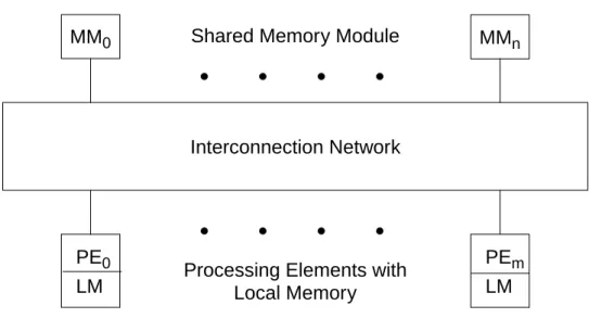
1.2.4 Interconnection Networks

Architectural models for a multiprocessor can be classified as being tightly cou-pled or loosely coucou-pled [Hwa84]. Tightly coucou-pled multiprocessors communicate through a shared main memory. Hence the rate at which data can be communicated from one pro-cessor to the other is on the order of the bandwidth of the memory. A small local memory or high speed buffer (cache) may exist in each processor (figure 1.5). Loosely coupled multiprocessors (also called multicomputers) communicate by passing messages. Again the performance and scalability of the multiprocessor is primarily determined by the interconnection network. The general structure for loosely coupled multiprocessors is

Figure 1.5 The general structure of tightly coupled multiprocessors.

MM₀ MM_n

Interconnection Network

LM LM

PE₀ PE_m

Shared Memory Module

Processing Elements with Local Memory

shown in figure 1.6.

Interconnection networks have been reviewed in many surveys [Fen81][Ree87] [Wit81]. The network topologies tend to be regular and can be grouped into two catego-ries: static and dynamic [Fen81]. In a static topology, links between two processors are passive and can not be reconfigured. On the other hand, links in the dynamic topology can be reconfigured by setting the networks’s active switching elements.

Though different authors use different methods to characterize the performance of the static topologies, some common measures are widely accepted [Bhu84][Ree87][Wit81]: they are:

1. average message traffic delay (mean internode distance), 2. average message traffic density per link,

3. number of communication ports per node (degree of a node), 4. number of redundant paths (fault tolerancy),

5. and ease of routing (ease of distinct representation of each node).

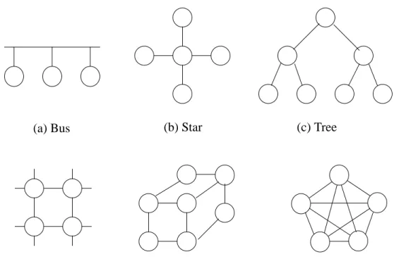
A multitude of different topologies compromise these measures, offering a wide range of cost/performance choices. Typical topologies are shown in figure 1.7.The com-pletely connected network with N processors has N-1 connections per node, so it is not suitable for even a moderate number of multiprocessors despite being optimal by all other

Figure 1.6 The general structure of loosely coupled multiprocessors

Interconnection Network

LM LM

PE₀ PE_m

Processing Elements with Local Memory

criteria. The simplest topology is the single shared-bus topology (e.g. Sequent Balance). Although the single bus topology is quite reliable and relatively inexpensive, it is not tol-erant of a malfunction in any of the bus interface circuitry. Moreover, system expansion, by adding more processors or memory, increases the bus contention, which degrades sys-tem throughput. To provide more communication bandwidth than by a single bus, multi-ple bus architectures (e.g. Pluribus) and hierarchical structures with clusters connected by a inter-cluster bus (e.g. Cm*) have been developed. These architecture pay for the increase bandwidth with more complicated bus arbitration logic. The bus bottleneck problem limits the size of multiprocessors with bus topology (typically < 20).

General agreement on the order of magnitude of the average message traffic delay and the average message traffic density is the order of the number of the processors

(b) Star (c) Tree

(d) Mesh (e) Binary hypercube (f) Completely connected (a) Bus

(O(logN)). There are some known network topologies satisfying this order: cube-con-nected-cycle [Pre81], lens [Fin81], dual-bus-hypercube[Wit81], generalized hypercube [Bhu84], and generalized nearest neighbor mesh [Wit81]. Among them, the binary hyper-cube, which is a special case of the generalized hypercube and also the generalized near-est neighbor mesh, is the most popular for moderate numbers of processors ranging from a few dozen to a few thousand processing elements (e.g. Intel iPSC, Ncube/10). The pri-mary disadvantage of the binary hypercube is that it requires a logarithmic increase in degree of a node as the total number of nodes increases. Other common topologies include star, mesh, tree and their variants.

Dynamic topologies are mainly used for tightly coupled multiprocessors to con-nect processors to the shared memory modules. There are three topological classes in the dynamic category: single-stage, multistage, and crossbar. Examples of dynamic network topologies are shown in figure 1.8.The shuffle-exchange network [Sto71] is the represen-tative single-stage network based on a perfect-shuffle connection cascaded to a stage of switching elements (e.g. NYU Ultracomputer). A multistage network consists of more than one stage of switching elements and is usually capable of connecting an arbitrary input terminal to an arbitrary output terminal. Depending on whether simultaneous con-nections of more than one terminal pair may result in conflicts in the use of the network communication links, multistage networks are further divided into three classes: block-ing, rearrangeable, and nonblocking [Fen81]. Various kinds of multistage networks have been implemented: omega (e.g. BBN Butterfly, IBM RP3), banyan, delta, Benes, and so on.

In a crossbar switch, every input port can be connected to a free output port with-out blocking. While this scheme yields a high processor/memory bandwidth, it incurs scaling problems due to a switching cost which increases as N2.

1.3. PARALLEL PROCESSING OVERHEADS

(a) Shuffle-exchange (single stage)

(b) Crossbar

(c) An 8x8 omega network (multistage)

Figure 1.8 Examples of dynamic network topologies

Regardless of what hardware architecture or software programming paradigm is used, there are many factors which limit the attainable speedup in a parallel processing environment.

1.3.1 Load Balancing

Load balancing is the primary concern for parallel processing. A proper load bal-ance distributes the computation load evenly across all of the processors to maximize effi-ciency, or to keep the processors busy as much as possible. A simple strategy to partition the actors with the same amount of total work usually results in a bad balance since some processors may be idled in case that the assigned actors are not executable. Therefore, the precedence relationship among actors should be taken into account. The finer the granu-larity of actors is, the less variance of the distributed workloads is expected. However, the load balancing scheme becomes more complicated due to the quadratic increase of prece-dence relations. Some dataflow machines were proposed to balance the loads at runtime with fine-grain dataflow graphs, which incur prohibitive runtime overhead of shipping codes across the interconnection network.

Another crucial issue, but often neglected in the literature, on load balancing is the dynamic (data-dependent) behavior of programs. For a program with dynamic behav-ior, there is no fixed partitioning which is best for all of the different runtime behaviors of the program.

1.3.2 Interprocessor Communication

Interprocessor communication is also a significant source of the extra overhead. It involves not only the communication delay required to transfer data between the source and destination processors but also involves the arbitration delay to acquire this access

privilege to the interconnection network. The common technique to compensate for this overhead is to use a split transaction scheme with dedicated hardware for network access. The overhead can be hidden effectively if the processors are kept busy with other runna-ble actors during the transactions. This is the main advantage of fine-grain dataflow machines, because they usually have a sufficient number of runnable actors through full exploitation of parallelism.

The arbitration delay is non-deterministic and depends on the network congestion and the arbitration strategy. The primary objective of an arbitration strategy is to reduce the possibility of an extraordinarily long latency. One interesting approach is to random-ize the memory access pattern for multistage dynamic networks. Excessive contention for a particular memory module in a dynamic network has been found to cause so-called “hot-spots” in the network, which are analogous to traffic jams. Since regular access pat-terns are more likely to cause these hot-spots, randomization destroys the regularity of access patterns, and so reduces the possibility of excessive contention according to prob-ability theory.

Communication delay depends on the amount of data transmitted. Therefore, a pair of actors with large communication requirements should be assigned to the same processor. Thus, there is a conflict between reducing communication requirements and load balancing. Communication delay also depends on the length of the path. For static networks, data must typically be routed through intermediate nodes before reaching its final destination. In this case, the physical network topology as well as communication requirements affects the efficiency of the partitioning, which makes the problem of find-ing the optimal partitionfind-ing even more intractable.

There are two possible partitioning strategies based on heuristic rationales. The unified strategy incorporates the effect of physical processor connectivity on communica-tion delay when particommunica-tioning [Sih91]. The other, called two-phase strategy, divides the

scheduling problem into two phases.

1. Partition the program ignoring the specific communication network topology of the target machine.

2. Assign the partitioned actors to the physical processors.

Once the first phase is done, the communication requirements for each pair of par-titions are determined. The objective of the second phase is to minimize the total commu-nication delays, or message traffic. A message traffic on a link is defined as the volume of data exchanged through the link. The total message traffic is the sum of message traffics on all links. Define v_ijand d_ij as follows.

v_ij- the volume of data exchanged between processor i and j.

d_ij - the number of links on the shortest path between processor i and j. Then the total message traffic becomes

(1-1) The problem of minimizing the total message traffic is well known as the qua-dratic assignment problem [Han72]. M. Hanan et. al. reviewed three techniques for the placement of logic packages: constructive-initial-placement, iterative-improvement, and branch-and-bound. While they did not consider network congestion, S. Lee and J. K. Aggarwal [Lee87] formulated a set of new object functions quantifying the effect of con-gestion based on deterministic information of when each communication occurs and with how much volume. The problem of minimizing network congestion with a given assign-ment may be attacked separately as the traffic scheduling problem [Bia87].

We examine the expected performance improvement we can achieve from the optimal assignment compared with a random assignment in the appendix. The analysis shows that the average performance improvement is about 20% to 30% ignoring the effects of the network congestion. Sih reported that the unified strategy can give higher

v_ijd_ij

i j,

∑

performance improvement since it can reduce the quantities { } [Sih91].

1.3.3 Other Factors

The local memory of a processor is limited in size so the number of active invoca-tions of actors should be limited accordingly. In dataflow machines, the number of activi-ties may grow indefinitely unless the degree of parallelism is restricted. It may create a deadlock condition when the local memory is filled with the contexts of the current activ-ities. Therefore, it is a challenging task to manage limited resources without sacrificing too much of the parallelism for dataflow machines.

Various forms of synchronization are necessary to allow cooperation between processors, creating additional overhead. The amount of overhead depends on which scheduling scheme is used, which will be discussed in the next chapter.

1.4. TARGET APPLICATION: DIGITAL SIGNAL PROCESSING

So far, we have reviewed program representations and multiprocessor architec-tures for general purpose applications. Program representations and multiprocessor archi-tectures are closely related. For conventional multiprocessors, fine-grain dataflow graphs has been proven very inefficient. Therefore, parallel languages of von Neumann type are preferred in spite of their shortcomings, such as difficulty in programming and debug-ging. The merits of fine-grain dataflow graphs come into life only with dataflow machines. Dataflow machines, however, are still immature and possess some difficulties, such as resource management and compatibility with conventional languages, to be over-come before they are commercially viable. Between these two extremes, there is large-grain dataflow (LGDF) which has gained little attention for general purpose applications.

In this dissertation, we focus on digital signal processing (DSP) applications. d_ij

They differ significantly from general purpose computations in that they are consistently numerically intensive, and many are real-time meaning that the full set of input data is not available before output data must be computed. In particular, for most such applica-tions, algorithms are repetitively applied to an essentially infinite stream of input data. Also, runtime behavior is mostly deterministic. These characteristics of DSP applications are efficiently exploited by a combination of LGDF representation and conventional mul-tiprocessors.

Digital signal processing algorithms are usually described in the literature by block diagrams consisting of functional blocks connected by dataflow paths. The blocks represent signal processing subsystems such as digital filters, FFT units, or adaptive equalizers. Each block may itself represent another block diagram, so the specification is hierarchical. This is consistent with the general practice in signal processing where, for example, a phase locked loop may be treated as a block in a large system, and may be itself a network of simpler blocks. In this case, block diagrams are large grain dataflow graphs.

Many block diagram system specifications have been developed to permit users to implement signal processing algorithms more naturally [Lee87b]. They differ in some description details but they use a common data-driven paradigm. Among them, we con-centrate on the synchronous dataflow (SDF) graph and its extension, the dynamic data-flow (DDF) graph.

1.4.1 Synchronous Dataflow Graph

Synchronous Dataflow (SDF) is a special case of data flow (either fine-grain or large-grain) in which the number of data samples produced and consumed by each node on each invocation is specified a priori [Lee87b]. An example of an SDF graph is shown below in figure 1.9. The numbers at the tail and head of each arc indicate the number of

data samples consumed and produced by the respective nodes. For example, node B con-sumes two data samples from node A and one data sample from node D, and produces one data sample to node C. The inscription 1D on the arc between node C and D indicates the presence of a delay in the signal processing sense, corresponding to a sample offset between the input and the output. In other words, the nth sample consumed by node D will be the (n-1)th sample produced by node C. This implies that the first sample D con-sumes is not produced by C at all, but is part of the initial state of the arc’s first-in first-out (FIFO) buffer. This initial data sample is necessary to avoid the deadlock condition, where each node waits for data from its predecessor.

Systems where all sample rates are rational multiples of all other sample rates are called synchronous in the signal processing literature. Synchronous DSP systems are eas-ily described using the SDF paradigm, hence the name for the paradigm. For example, a 2:1 decimator node would have one input and one output, but would consume two tokens for every token produced. Thus, relative sample rates are represented by the numbers attached to the input or output arcs of nodes. One requirement of SDF graphs is that sam-ple rates should be consistent. Inconsistent samsam-ple rates can lead to deadlock, or unbounded memory requirements. Consistency is defined to mean that the same number of tokens are consumed as produced on any arc, in the long run. A systematic method for consistency checking was developed for SDF graphs [Lee87b], and generalized further

2 1 1 1 1 2 1 1 1 1 1D A B C D E

for dataflow languages [Lee91b].

The most salient feature of the SDF paradigm is that the execution order of nodes can be determined at compile-time. Moreover, if the execution time of each node is known and fixed beforehand, nodes can be partitioned optimally at compile-time. Dead-lock avoidance and bounded memory requirements can also be guaranteed at compile-time. As a result, the runtime supervisory overhead can be replaced with the correspond-ing compiler task. Recall that dataflow architectures are required to preserve the merits of dataflow graphs for general purpose applications. However, they seem to be unnecessary for SDF graphs, because what they do in hardware can be done at least as well by a com-piler at much lower cost. Many researchers follow this line: translate block diagram descriptions of signal processing algorithms into run-time code for multiple programma-ble DSP processors of von Neumann type [Lee89a][Zis87][Tha90].

SDF graphs consist only of synchronous actors where the number of tokens pro-duced and consumed must be independent of the data. Most nodes for signal processing applications are synchronous and this synchrony is taken advantage of through compile-time analysis. However, the SDF paradigm is too restrictive to express general signal pro-cessing applications. Dynamic dataflow graphs overcome this difficulty by allowing asynchronous actors in the specification.

1.4.2 Dynamic Dataflow Graph

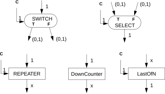
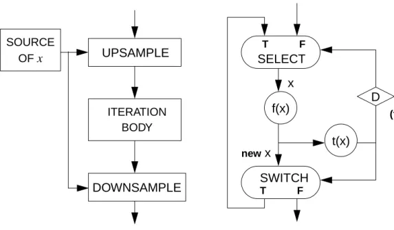
Some asynchronous nodes are shown in figure 1.10. The SWITCH node con-sumes one data input from the input arc and one boolean input from the control arc, C. Depending on the Boolean value received from the control arc, it produces one output either to the true arc,T, or to the false arc,F. The number of data samples produced on the two outputs, therefore, is data-dependent. On the contrary, theSELECT node consumes one input either from the true arc or from the false arc, depending on the boolean value

received from the control arc. The figure also illustrates two data-dependent up-sample nodes and one data-dependent down-sample node. The number of data samples produced on the output arc of theREPEATER is determined by the control value, hence it is data-dependent. The DownCounter node generates down-counted integer samples starting from the value of the input sample. The LastOfN node consumes x input samples and produces one output sample, where x is determined by the control value received from the control arc. Dynamic dataflow (DDF) graphs consist of both asynchronous nodes and synchronous nodes [Lee88][Buc91a]. By using asynchronous nodes, the DDF paradigm can represent the well-known dynamic constructs such as if-then-else, for-loop, and do-while-loop; thus it overcomes the main modeling limitation of the SDF paradigm (figure 1.11). In figure 1.11 (b), the diamond containing D on the arc connected to the control input of the SELECT node represents a logical delay, or an initial data sample. The ini-tial Boolean value should be “false” so that the first token selected comes from the out-side, rather than from the feedback loop.

SWITCH T F C 1 1 (0,1) (0,1) SELECT T F C 1 1 (0,1) (0,1) REPEATER 1 C 1 x LastOfN x C 1 1 DownCounter 1 x

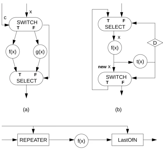
Dynamic dataflow graphs sacrifice the run-time efficiency of SDF graphs for the enhanced modeling power. The execution order of the nodes of a DDF graph can not be fully specified at compile-time. For example, in the if-then-else construct in figure 1.11 (a), either the f(x) node or theg(x) node is fired after the SWITCH node, depending on the control value,c, which is known at run-time only. The requirement of runtime deci-sion making turns some researchers’ attention to dataflow digital signal processors like dataflow machines for general applications: the Hughes Dataflow Machine (HDFM)

Figure 1.11 Dynamic dataflow graphs that model some familiar dynamic constructs: (a) if c then f(x) else g(x), (b) do x = f(x) while t(x), and (c) for (i = c; i > 0; i--) f(x).

SWITCH T F SELECT T F f(x) g(x) x c REPEATER _f(x) LastOfN c x (a) (c) SELECT T F f(x) SWITCH T F t(x) (b) D new x x

[Gau85], the NEC uPD7281. [Cha84] and so on. Dataflow DSPs, however, are operated by fine-grain dataflow graphs, which again possess the same difficulties as the general purpose dataflow machines discussed earlier. J. Gaudiot [Gau87] concludes that dataflow DSPs find their applications in problems which involve large amounts of heuristics and decision making.

Digital signal processing algorithms provide a unique set of opportunities; they often have predictable, or mostly predictable control flow. The overhead of dataflow DSPs seems too high a price to pay to manage a small amount of run-time decision mak-ing. A challenging research area is to incorporate decision making capability and at the same time preserve the efficiency of dataflow execution in multiple conventional DSPs of von Neumann style.

1.5. CONCLUSION

At least for signal processing applications, data-driven principles of execution are a necessity in the design of multiprocessor systems, be they incorporated at compile or runtime. The granularity of parallelism presents a trade-off between managing dynamic behavior and utilizing highly efficient sequential, control-flow execution. The optimal granularity, therefore, is application-specific. In particular, many digital signal processing applications match well with large-grain dataflow graphs. Regardless of what hardware architecture or software programming paradigm is used, there are fundamental difficul-ties that arise when using multiple processors: load balancing and communication over-head. The efficient coordination of processors requires both a program partitioning and a scheduling strategy. In this dissertation, we focus on applications that have at most a small amount of data-dependent behavior, which covers most signal processing applica-tions and computation-intensive applicaapplica-tions. Since we make no restriction here about the

granularity of the dataflow graph, the proposed techniques are valid both for fine-grain and large-grain even though we assume large-grain dataflow graphs throughout the dis-sertation.

SCHEDULING

2

For you yourselves know how you ought to follow us, for we were not disorderly among you; ... Not because we do not have authority,

but to make ourselves an example of how you should follow us. --- II Thessalonians 3:17,19

The processor scheduling problem is to map a set of precedence-constrained tasks {T_i} i = 1 ... n, onto a set of processors {P_k}, k = 1 ... p in order to satisfy a specified objective. An acyclic precedence graph is commonly used to describe the interrelation-ships among tasks where an arc A_ijdirected from task T_ito T_jindicates that T_imust pre-cede T_j in execution. While processor scheduling has a very rich and distinguished history [Cof76] [Gon77], most efforts have been focused on deterministic models, where the execution time of a task T_i on a processor P_k is fixed and there can be no conditional (data-dependent) nodes in the program graph.

There are a number of factors that can be gauged to classify the scheduling tech-niques: task interruptibility, deadlines, processor homogeneity, and so on [Gon77]. If the

interruption (and subsequent resumption) of a task before its completion is permitted, we speak of preemptive scheduling. In nonpreemptive scheduling, any task which has started execution on a processor must be completed. Preemptive scheduling should consider the context-switching overhead to assess the gain of preemption. Ignoring that overhead, pre-emptive scheduling generates schedules that are better than those generated by nonpre-emptive scheduling. In this thesis, we restrict our attention to nonprenonpre-emptive scheduling.

In real-time applications, deadlines or scheduled completion times may be estab-lished for individual tasks T_i. If the deadlines are enforced for each execution, we speak of a hard real-time schedule. In a soft real-time schedule, the deadline requirement is based on a statistical distribution of terminations. We exclude hard real-time disciplines throughout the thesis. We also assume that the processors are all identical.

Deterministic schedules are usually displayed with timing diagrams known as Gantt charts as shown in figure 2.1. In this schedule, three processors are involved. The tasks assigned to each processor and their order of execution and execution time require-ments are represented by the horizontal lines and task identifications. The dark area rep-resents the idle time of the associated processor.

A B C D E F G 0 1 2 3 4 5 6 time Processor 1 2 3

2.1. SCHEDULING OBJECTIVES

A program graph may be executed only once, or repeated at irregular intervals over a long period of time. The scheduling objective, in this case, is either (1) to minimize the finishing time, also called makespan, of the program with a given number of proces-sors, or (2) to minimize the number of processors required to process the program in the smallest possible time [Ram72]. A program graph is first converted to a homogenous dataflow graph, and finally to an acyclic precedence graph. The second conversion is accomplished by splitting ideal delays into a pair of input and output nodes. The output node is connected to the source node of the removed arc, and the input node is connected to the destination node of the arc. Then, the smallest possible time is nothing but the longest path, called critical path, in terms of computational delay between inputs and outputs in a given acyclic precedence graph. In multiprocessor scheduling, the number of processors is fixed, so we focus on minimizing the finishing time of a given program.

In most DSP applications, however, the program is executed once for every sam-ple of an input stream. For such iterative executions, the objective is to maximize the throughput or to minimize the iteration period. A tightest lower bound on the iteration period, referred as the iteration period bound, can be obtained from a dataflow graph [Ren81]. The iteration period bound ( ) is

, (2-1)

where n_lis the total delays in loop l, d_j is the execution time of the j th node on the l th loop, and D_l represents the total execution time of the l th loop. The quantity inside the brackets {D_l / n_l} is called the loop bound, T_l. The loops which have the largest loop

T_o T_o

max

∑

bound are called the critical loops. The critical loops determine the iteration period bound of a dataflow graph. A schedule that achieves the iteration period bound is said to be rate optimal.

If the number of processors is not fixed, another possible objective is to minimize the required number of processors to implement a rate optimal schedule, which is lower bounded by the processor bound, P_o:

, (2-2)

where D is the total execution time of the program executed sequentially, and T_o is the iteration period bound. The processor bound may not be attainable since the above for-mula ignores precedence constraints although it enforces load balancing. A processor optimal schedule uses the minimum number of processors possible.

In addition to rate and processor optimality criteria, delay optimality can also be defined. A delay optimal schedule minimizes the time delay between a pair of input and output nodes. Another indirect measure of performance is the processor efficiency which is defined as the ratio of the average busy time of the processors to the iteration period. For a rate optimal schedule, the difference between 100% and the true processor effi-ciency is called the inherent processor ineffieffi-ciency.

2.1.1 Blocked Schedule

Although we are interested in iterative execution cases, we aim to minimize the makespan as the scheduling objective assuming that the whole system is committed to one execution at a time. This falls under the category of non-overlap execution schedul-ing accordschedul-ing to P. Hoang [Hoa90]. We construct a blocked schedule where each iteration cycle terminates before the next cycle begins. The iteration period becomes the length of

P_o D T_o ---= D d_j j

∑

one cycle of a blocked schedule, which is also the reciprocal of the throughput. Certainly, the non-overlap execution schedule does not guarantee the rate-optimal realization because it places artificial boundaries between iterations of the graph. On the other hand, overlap execution scheduling allows overlapped execution of successive iterations. A comparison of these two categories is illustrated in figure 2.2. When a blocked schedule

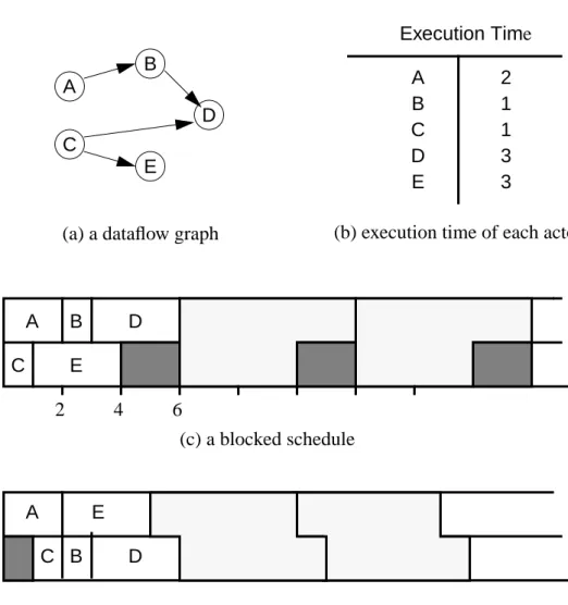
A B D C E Execution Time 2 1 1 3 3 A B C D E

(a) a dataflow graph (b) execution time of each actor

(c) a blocked schedule

(d) an overlap execution schedule

A B D C E A C B E D

Figure 2.2 A comparison of a blocked schedule and an overlap execution schedule. (a) A dataflow graph has two input actors and two output actors whose execution times are shown in (b). A blocked schedule (c) is made so that the iteration period is 6 time units, and each period has 2 idle time units on the second processor. An overlap execution schedule (d) shows the optimal throughput, 5 time units.

is constructed, all processors are synchronized after each cycle of iteration so that the pat-tern of processor availability is flat before and after each cycle (meaning that all proces-sors become available for the next cycle at the same time). As a result, the second processor is padded with no-ops, two time units of idle time. On the other hand, the opti-mal throughput is achieved by an overlap execution schedule. At the sixth time unit, the first processor begins execution of the next iteration with actor A, while the second pro-cessor is still processing actor D of the current iteration. The main motivation of using blocked scheduling is to reduce the computational complexity of scheduling.

However, it is possible to improve the throughput performance of a nonoverlap execution schedule. One technique we may use is loop winding [Gir87], which basically pipelines the program graph. In spite of mapping pipeline stages into a pipeline structure of hardware, it shares processors between stages to achieve a functional pipeline. The retiming [Lei83] technique can be used for optimal pipelining [Pot91]. Retiming was originally developed to alter the clock period of a synchronous circuit by relocating regis-ters. The retiming transformation is performed on the dataflow graph before it is con-verted to the acyclic precedence graph. If a graph contains cycles, the iteration period is limited by the iteration period bound. Retiming provides a systematic method for trans-forming a graph so that the iteration period approaches this bound. In iterative execution cases, the whole graph can be thought of as the body of a cycle. By adding dummy input and output nodes and connecting them with some delays, the graph becomes ready for the retiming transformation. An example of the retiming transformation and the resulting schedule are shown in figure 2.3. Note that after the retiming transformation, the original dataflow graph is functionally pipelined. In the dataflow context, the delays represent ini-tial data samples, which should be provided beforehand. For instance, the first iteration cycle could be processed to produce the initial samples before processing the retimed graph. Or, we can make a schedule preamble of actors A, C in figure 2.3 for example.

After scheduling actors A, C as a preamble, we schedule actors B, D, E of the current execution cycle and actors A, C of the next execution cycle using blocked scheduling. Instead of applying the retiming transformation, in practice, the programmer may insert delays on a certain cutset of the graph to realize a functional pipeline to expose more par-allelism between iterations.

It may be possible to expose the hidden parallelism between iterations by increas-ing the blockincreas-ing factor. The blockincreas-ing factor corresponds to how many iterations are expressed in a program graph. If we assume that successive invocations of the same actor can not overlap in time, the new dataflow graph with blocking factor 2 and the corre-sponding blocked schedule becomes as displayed in figure 2.4. The figure illustrates that by increasing the blocking factor the throughput can be increased in many cases. In this

Figure 2.3 (a) A dummy input node and a dummy output node connected with a unit delay are added to a graph. (b) The graph of (a) is retimed. (c) The blocked sched-ule of the retimed graph shows the optimal throughput in this example.

A B D C E In Out D (a) A B D C E In Out D D D (b) retimed graph (c) a blocked schedule A D C E 2 4 6 B

particular example, the corresponding blocked schedule produces the optimal schedule. The costs incurred by an increasing blocking factor are two-fold; more memory is required in each processor to store the longer schedule, and scheduling will take longer because more nodes are present in the acyclic precedence graph. To our knowledge, the problem of finding the optimal blocking factor is still open except a special case, in which the execution time of each actor is the same, or unity [Cha92].

Sometimes, the program graph can be modified by changing the algorithm; digital filters for instance to reduce the iteration period bound [Par89a][Par89b].

2.2. A SCHEDULING TAXONOMY

The Scheduling of parallel computations consists of assigning actors to

proces-Figure 2.4 (a) A dataflow program graph derived from figure 2.2 (a) by increasing the blocking factor to 2. (b) The optimal blocked scheduling optimizes the throughput in this case. It shows that increasing the blocking factor is a way to increase the throughput of a nonoverlap execution schedule.

A₁ B₁ D₁ C₁ E₁ A₂ B₂ D₂ C₂ E₂ (a) (b) a blocked schedule A₁ B₁ C₁ E₁ 2 4 6 E₂ A₂ B₂ C₂ D₁ D₂

sors, specifying the order in which actors fire on each processor, and specifying the time at which they fire. These tasks can be done either at compile time or at run time. Depend-ing on which operations are done when, we define four classes of schedulDepend-ing, depicted in figure 2.5.

The first type is fully dynamic, where actors are scheduled at run time only. When all input operands for a given actor are available, the actor is assigned to an idle processor and fired. The second type is static assignment, where an actor is assigned to a processor at compile time and a local run-time scheduler invokes actors assigned to the processor based on data availability. In the third type of scheduling, the compiler determines the order in which actors fire as well as assigning them to the processors. At run-time, the processor waits for data to be available for the next actor in its ordered list, and then fires that actor. We call this self-timed scheduling because of its similarity to self-timed cir-cuits. The fourth type of scheduling is fully static; here the compiler determines the exact firing time of actors, as well as their assignment and ordering. This is analogous to syn-chronous circuits. As with any taxonomy, the boundary between these categories is not rigid. Self-timed scheduling and fully static scheduling are both called static scheduling.

RUN RUN RUN

RUN RUN

RUN

COM-COM-

COM-COM- COM-

COM-assignment ordering timing

fully dynamic static-assignment

self-timed fully static

Figure 2.5 The time which the scheduling activities “assignment”, “ordering”, and “tim-ing” are performed is shown for four classes of schedulers. The scheduling activi-ties are listed on top and the strategies on the left [Lee89b].

We can give familiar examples for each of the four strategies applied in practice. Fully dynamic scheduling has been applied in the MIT static dataflow architecture [Den80], the LAU system, from the Department of Computer Science, ONERA/CERT, France [Pla76], and the DDM1 [Dav78]. It has also been applied in a digital signal pro-cessing context for coding vector processors, where the parallelism is of a fundamentally different nature than that in dataflow machines [Kun87]. A machine that has a mixture of fully dynamic and static-assignment scheduling is the Manchester dataflow machine [Wat82]. Here, 15 processing elements are collected in a ring. Actors are assigned to a ring at compile time, but to a PE within the ring at run time. Thus, assignment is dynamic within rings, but static across rings.

Examples of static-assignment scheduling include many dataflow machines [Sri86]. Dataflow machines evaluate dataflow graphs at run time, but a commonly adopted practical compromise is to allocate the actors to processors at compile time. Many implementations are based on the tagged-token concept [Arv82]; for example TI’s data-driven processor (DDP) executes Fortran programs that are translated into dataflow graphs by a compiler [Cor79] using static-assignment. Another example (targeted at digi-tal signal processing) is the NEC uPD7281 [Cha84]. The cost of implementing tagged-token architectures has recently been dramatically reduced using an “explicit tagged-token store” [Pap88]. Another example of an architecture that assumes static-assignment is the pro-posed “argument-fetching dataflow architecture” [Gao88], which is based on the argu-ment-fetching data-driven principle of Dennis and Gao [Den88].

When there is no hardware support for scheduling (except synchronization primi-tives), then self-timed scheduling is usually used. Hence, most applications of today’s general purpose multiprocessor systems use some form of self-timed scheduling, using for example Communicating Sequential Processes (CSP) principles [Hoa78] for synchro-nization. In these cases, it is often up to the programmer, with meager help from a

com-piler, to perform the scheduling. A more automated class of self-timed schedulers targets wavefront arrays [Kun88]. Another automated example is a dataflow programming sys-tem for digital signal processing called Gabriel that targets multiprocessor syssys-tems made with programmable DSPs [Lee89a]. Taking a broad view of the meaning of parallel com-putation, asynchronous digital circuits can also be said to use self-timed scheduling.

Systolic arrays, SIMD (single instruction, multiple data), and VLIW (very large instruction word) computations [Fis84] are fully statically scheduled. Again taking a broad view of the meaning of parallel computation, synchronous digital circuits can also be said to be fully statically scheduled.

As we move from fully dynamic to fully static, the compiler requires increasing information about the actors in order to construct good schedules. However, assuming that the information is available, the ability to construct deterministically optimal sched-ules increases. The domain of a scheduling strategy can be loosely defined as the set of algorithms for which the scheduling strategy does well. The range is the set of architec-tures that the strategy can target well. Most practical scheduling strategies have a limited domain or range.

2.2.1 Fully Static Scheduling

Of the classes we have defined, fully static scheduling has the narrowest domain. The subclass of dataflow graphs for which fully static scheduling works best is synchro-nous data flow [Lee87a] with all actors having known execution times. Unfortunately, even in this restricted domain, algorithms that accomplish such optimal scheduling have combinatorial complexity, except in certain trivial cases [Cof76][Cap84]. Therefore, good heuristic methods have been developed over the years. The typical approach is based on list scheduling, in which actors are assigned priorities and placed in a list and executed in order of decreasing priority [Ada74][Cof76][Sih90b]. Other approaches such

as clustering [Kim88][Sar87], declustering [Sih91] and 0-1 integer programming [Kon90] also have been proposed. These heuristics all aim to minimize the schedule length (makespan of the program). This approach is adequate for latency-sensitive appli-cations or in situations where barrier synchronization between iterations of the schedule is required.

In most DSP applications, however, the program is executed once for every sam-ple of an input stream. As a result, by overlapping executions of successive iterations, the computational throughput can be improved. Typical approaches are based on cyclo-static scheduling [Sch85][Gel91], which is rate, processor and delay optimal. However, the exponential worst-case running time of the scheduling algorithm, the lack of consider-ation for resource constraints and the extensive communicconsider-ation requirements preclude a practical implementation, possibly except for simple structures such as digital filters. Chain partitioning [Bok88] represents another technique based on pipelining serial tasks on a linear array of processors to maximize throughput; Its domain is again quite limited. Recently, a heuristic that simultaneously considers pipelining, retiming, parallelism and hierarchical node decomposition has been proposed as part of a software environment for partitioning DSP programs onto a configurable multiprocessor system [Hoa90].

The range depends on the sophistication of these methods, although most straightforward implementations target homogeneous tightly coupled multiprocessors with full interconnectivity. The requirement for full interconnectivity limits the range to machines with modest parallelism.

A subclass of fully static scheduling is the set of techniques based on projecting dependence graphs for regular iterative algorithms onto systolic arrays [Kun88] [Rao85]. These techniques have a very limited domain (RIA’s) and range (systolic arrays), but do extremely well within these constraints.

Since behavior is completely known at compile time, there is no need to check at run time to see when actors can be fired. The compiler can figure it out, so actors simply fire at the designated time, and are assured that their data is available.

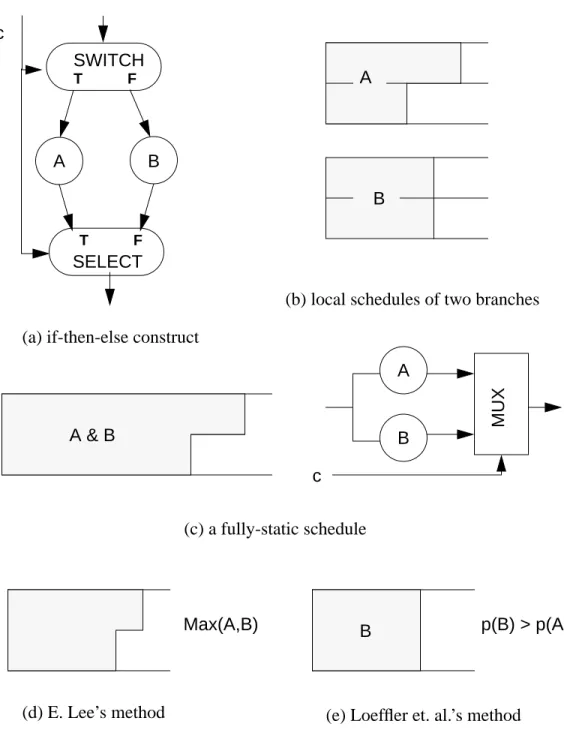
The domain of static scheduling specifically does not include dataflow graphs with actors that have data-dependent execution times or actors that may or may not fire, depending on the value of some data somewhere in the graph. These restrictions are severe, since they exclude both conditionals and data-dependent iteration within an actor or involving several actors. The restrictions can be relaxed, however, at the expense of optimality in the resulting schedule. For example, an actor with a data-dependent execu-tion time can be padded so that it always executes in worst-case time. This is not so bad when the application has hard real-time constraints, but otherwise may be very costly. As another example, to implement the synchronous dataflow equivalent of if-then-else, both branches of the conditional may be computed, and the desired result may be selected. There are again applications where this option is acceptable, for example when one of the two conditional branches is trivial, but most of the time the cost will be high. The concept of static scheduling has been extended to solve some of these problems, using a technique called quasi-static scheduling [Lee88]. In quasi-static scheduling, some firing decisions are made at run-time, but only where absolutely necessary.

2.2.2 Self-Time Scheduling

Self-timed scheduling has a slightly broader application domain than fully static scheduling. Although the order of execution of actors is fixed for each processor at com-pile time, the exact firing times are not. Consequently, the schedule can automatically compensate for certain fluctuations in execution times. For example, if one actor finishes earlier than expected, the following actor can fire immediately, as long as its data is avail-able. This means that the second actor can finish later than expected without any loss in <