Dissecting Network Externalities in International Migration

Dissecting Network Externalities

in International Migration

Michel Beine

Frédéric Docquier

Ça

ğ

lar Özden

CES

IFO

W

ORKING

P

APER

N

O

.

3333

C

4:

L

M

J

2011

An electronic version of the paper may be downloaded

• from the SSRN website: www.SSRN.com

• from the RePEc website: www.RePEc.org

CESifo Working Paper No. 3333

Dissecting Network Externalities

in International Migration

Abstract

Existing migrant networks play an important role in explaining the size and structure of immigration flows. They affect the net benefits of migration for future migrants by lowering assimilation costs (‘self-selection’ channel) and increase the probability of potential migrants to obtain a visa through family reunification programs (‘immigration policy’ channel). This paper presents an identification strategy allowing to disentangle these two channels. Then, it provides an empirical illustration based on US immigration data by metropolitan area and country of origin. First, we show that the overall network externality is strong: the elasticity of migration flows to network size is around one. Second, only a quarter of this elasticity is accounted for by the policy channel. Third, the policy channel was stronger in the nineties than in the eighties due to more generous family reunion program. Fourth, the global elasticity and the policy contribution are much greater for low-skilled migrants.

JEL-Code: F220, O150.

Keywords: migration, network/diaspora externalities, immigration policy.

Michel Beine University of Luxembourg

Luxembourg [email protected] Frédéric Docquier

Catholic University of Louvain Belgium

[email protected]

Çağlar Özden

World Bank, Development Research Group USA

[email protected]

December 22nd_{, 2010}

We thank Cristina Ileana Neagu for remarkable assistance and Suzanna Challen for providing precious information about the US immigration policy. The second author acknowledges financial support from the ARC convention on "Geographical Mobility of Factors" (convention 09/14-019). The findings, conclusions and views expressed are entirely those of the authors and should not be attributed to the World Bank, its executive directors or the countries they represent. This paper benefitted from comments of participants of the Swiss Economic Association (Freiburg, June 2010), the World Bank Trade seminar (Washington DC, August 2010), the Third .Migration and Development.Conference (Paris, September 2010), the Migration Conference (Ottawa, October 2010). We thank in particular A. Spilimbergo, S. Bertoli, T. Mayer, M. Schiff for useful comments and suggestions. Of course, the

1

Introduction

Even in the age of instant communication and rapid transportation, immigration to a new country is a costly endeavor. Migrants face signi…cant legal barriers, social adjustment costs, …nancial burdens and many uncertainties while they are trying reach and settle in their destinations. By providing …nancial, legal and social sup-port, existing diasporas or social networks a¤ect overall costs and bene…ts faced by new migrants. As a result, diasporas strongly in‡uence various aspects of migration patterns, especially with respect to the size, skill composition and destination choices. The goal of this paper is to identify and determine the relative importance of dif-ferent channels through which diasporas in‡uence migration patterns. These channels may be divided into two general categories. The …rst one, referred to as the ’self-selection’channel, is the lowering of assimilation costs which generally matter after

the migrant crosses the border. Assimilation costs cover a wide range of hurdles faced by the migrants in …nding employment, deciphering foreign social and cultural norms and adjusting to a new linguistic and economic environment. All of these obstacles tend to be local in nature and the the support provided by the existing local net-work can be crucial.1 _{The second channel, referred to as the ’policy’channel, is the}

overcoming of legal entry barriers and they help the migrant at the border before

she/he arrives at the …nal destination. Diaspora members who have already acquired citizenship or certain residency rights in the destination countries become eligible to sponsor their immediate families and other relatives. These family reuni…cation programs are the main routes for many potential migrants in most OECD countries. The overall e¤ect of diasporas have been clearly recognized in the sociology, de-mography and economics literatures and extensively analyzed over the last twenty years (such as Boyd, 1989). Regarding assimilation costs, Massey et al. (1993) pro-vided one of the earliest papers, showing show diasporas reduce moving costs, both at the community level (e.g. in‡ow of people from the same nation helps creating subcultures), and at the family level (increase utility of friends and relatives). As shown by Carrington, Detragiache and Viswanath (1996), this explains why the size and structure of migration ‡ows gradually change over time. In addition, networks provide information and assistance to new migrants before they leave and when they arrive; this facilitates newcomers’integration in the destination economy or reduces uncertainty. Based on a sample of individuals originating from multiple communities in Mexico and residing in the U.S., Munshi (2003) showed that an individual is more likely to be employed and earn higher wage when her network is larger.2 _{At the}

macro level, Beine et al. (2010) used a bilateral data set on international migration

1_{Bauer et al. (2007) or Epstein (2008) argued that network e¤ects might re‡ect ’herd behavior’}

in the sense that migrants with imperfect information about foreign locations follow the ‡ow of other migrants, based on the (wrong or right) supposition that they had better information.

2_{On the contrary, Piacentini (2010) used data on migration and education from a rural region}

of Thailand to show that networks negatively a¤ect the propensity of young migrants to pursue schooling while in the city.

by educational attainment from 195 countries to 30 OECD countries. They explored how diasporas a¤ect the size and human capital structure of future migration ‡ows. They …nd that the diasporas are by far the most important determinant, explaining over 70 percent of the observed variability of the size of ‡ows. Regarding selection, di-asporas were found to favor the migration of low-skilled relative to the highly-skilled, thus exerting a negative impact and explaining over 45 percent of the variability of the selection ratio. Using micro-data from Mexico, the earlier study of McKenzie and Rapoport (2010) found the same e¤ect, which is also supported by Winters et.al (2001).

In terms of the e¤ect of diasporas in overcoming policy induced migration re-strictions, family reuni…cation is the main legal route for many potential migrants in most continental European countries. Even in one of the most selective country such as Canada, about 40 percent of immigrants come under the family reuni…cation and refugee programs, rather than selective employment or skill-based programs (e.g. point systems). Jasso and Rosenzweig (1986, 1989) estimated that each U.S. labor-certi…ed immigrant generated a …rst-round multiplier around 1.2 within ten years (i.e. sponsored 0.2 relatives). Using a longer perspective, Bin Yu (2007) showed that each newcomer generates an additional in‡ow of 1.1 immigrant.

The goal of this paper is to empirically decompose the relative importance of these two channels - lowering of assimilation costs and overcoming policy induced legal barriers.

A natural approach is to directly use micro data on the various entry paths mi-grants use as well as their individual characteristics. Appropriate use of indicators on migration policies along with diaspora characteristics could provide information on the relative importance of kinship-based admission of new migrants. Unfortunately, there is, to the best of our knowledge, no large micro database providing detailed information on the various entry tracks migrants use as well as the corresponding ‡ows for each track. Furthermore, information on changes in immigration laws might not be enough to gauge the importance of family reuni…cation policies over time. For example, many illegal migrants became legal residents after amnesty programs took place in the US in the nineties. Those regularized migrants became eligible to bring their close relatives to the US. This resulted in an increase in the number of migrants coming through family reuni…cation in spite of no signi…cant change in US migration laws. Another issue is that a signi…cant number of highly skilled US migrants used kinship-based tracks for convenience while they were fully eligible to use economic mi-gration tracks such as H1B or special talent visas.3 _{Ascribing their migration pattern}

only to the family reuni…cation track would give a distorted picture of the importance of each migration channel.

As an alternative to the use of data on individual immigration paths, this paper develops a di¤erent identi…cation strategy using migration aggregate data available at

3_{Some well known scholars in the economic migration literature provide striking examples of that}

the city level for the United States.4 As mentioned earlier, the role of the diasporas in overcoming migration barriers operates at the border before the migrant settles in a given city. Thus, the probability for a migrant to obtain a visa through a family reuni-…cation program depends on thetotal size of the network already living in the United States, not on the distribution of the diaspora across di¤erent cities. On the other hand, the assimilation e¤ect is mostly local and matters after the migrant chooses a city. For example, if a migrant lives in New York, the diaspora in Los Angeles is less likely to be of much help to him in terms of …nding a job, especially relative to the network present in New York itself. This is the distinction we exploit to identify the relative importance of these two channels. We develop a simple theoretical model showing that, under plausible functional homogeneity of the two network externali-ties, the two di¤erent channels can be identi…ed using U.S. bilateral data by country of origin and by metropolitan area of destination. We then provide several extensions based on educational di¤erences, time dimension, alternative migrant de…nitions or geographic areas and control of potential endogeneity.

We …rst show that the overall network e¤ect is strong. The elasticity of migration ‡ows to networks is around one, a result in line with Bin Yu (2007) and Beine et.al. (2010). Second, only a quarter of this elasticity is accounted for by the policy channel; the rest is due to the assimilation e¤ect. On average, each immigrant sponsors 0.25-0.30 relative within ten years, a result in line with Jasso and Rosenzweig (1986, 1989). This shows the di¢ culty for host country government to curb the dynamics of immigration and con…ne multiplier e¤ects. Third, the policy-selection channel was higher in the nineties than in the eighties due to more generous family reunion programs. Fourth, the global elasticity and its policy contribution are greater for low skilled migrants. Finally, these results are extremely robust to the speci…cation, to the choice of the dependent variable, to the de…nition of the relevant network and to the instrumentation of network sizes.

The remainder of this paper is organized as following. Section 2 uses a simple labor migration model to explain our identi…cation strategy. Data are described and econometric issues are discussed in Section 3. Results are provided in Section 4. Finally, Section 5 concludes.

2

Model and identi…cation strategy

We use a simple model of labor migration where inviduals with heterogeneous skill types s (s = 1; :::; S) born in origin country i (i = 1; :::; I) decide whether to stay in their home country or emigrate to location j (j = 1; :::; J) in the destination country. In the estimation, the set of destination locations are di¤erent cities in the

4_{The US Census data is actually disaggregated at the metropolitan area level which might include}

multiple cities or a city and its surrounding areas. For simplicty, we use the phrase "city" instead of "metropolitan area."

same country, the United States, and, therefore share the same national immigration policy but they di¤er in other attributes. The individual utility is linear in income but also depends on possible migration and assimilation costs as well as characteristics of the city of residence. The utility of a type-s individual born in countryi and staying in country i is given by

us_ii=w_is+As_i +"ii

where w_is denotes the expected labor income in location i, Ai denotes country i’s

characteristics (amenities, public expenditures, climate, etc.) and"ii is an

individual-speci…c iid extreme-value distributed random term. The utility obtained when the same person migrates to location j is given by

us_ij =w_js+A_js C_ijs V_ijs+"ij

where ws

j, Asj and "ij denote the same variables as above. In addition, two types of

migration costs are distinguished as in Beine et al. (2010). On the one hand, Cij

captures moving and assimilation costs that are borne by the migrant. Cs

ij, together

with (ws

j +Asj) (wis+Asi), would determine the net bene…t of migration in a world

without any policy restrictions on labor mobility and the self-selection of migrants into destinations. We will assume below thatCij depends on the network size in location

j. The network outside j, on the other hand, has no e¤ect on the migrants moving toj. Next,Vs

ij represents policy induced costs borne by the migrant to overcome the

legal hurdles set by the destination country’s government’s (policy channel). Since family reunion programs are implemented at the national level, Vs

ij depends on the

network size at the country level, not at the city level. Obviously, the main motivation to di¤erentiate between these two types of costs is to identify the role of immigration policy on the size and structure of migration ‡ows.

For simpli…cation, we slightly abuse the terminology and refer to Cs

ij as local

moving/assimilation costs and to Vs

ij as national visa costs. It is worth noting

that we allow both of these costs to vary with skill type. It is well documented that high-skill workers are better informed than the low skilled, have higher capacity adapt to assimilate or have more transferrable lingusitic, technical and cultural skills (see for instance Grogger and Hanson, 2010). In short, high skilled workers face lower assimilation costs. In addition, the skill type also a¤ects visa costs if there are selective immigration programs (such as points-system in Canada, Australia, New-Zealand, UK, the H1-B program in the US, etc.) that speci…cally target highly educated workers and grant them special preferences.

LetNs

i denote the size of the native population of skill s that is within migration

age in country i. When the random term follows an iid extreme-value distribution, we can apply the results in McFadden (1974) to write the probability that a type-s

individual born in country iwill move to location j as

Prhus_ij = max k u s ik i = N s ij Ns i = exp w s j +Asj Cijs Vijs P kexp [wks+Ask Ciks Viks] ;

and the bilateral ratio of migrants in city j to the non-migrants is given by Ns ij Ns ii = exp w s j +Asj Cijs Vijs exp [ws i +Asi]

Hence, the log ratio of emigrants in city j to residents of i (Ns

ij=Niis) is given by the following expression ln N s ij Ns ii = ws_j w_is + As_j As_i C_ijs +V_ijs (1)

Let us now formalize network externalities. As stated above, both Cs

ij and Vijs

depend on the existing network size. Local moving/assimilation costs depend on origin country and host location characteristics (denoted by cs

i and csj respectively),

increases with bilateral distance dij between i and j, and decreases with the size of

the diaspora network at destination,Mij (captured by the number of people living in

locationj and born in country i) at the time of migration decision of our individual. In line with other empirical studies, we assume logarithmic form for distance and diaspora externality, and add one to the network size to get …nite moving costs to destination where the network size is zero. This leads to

C_ijs =cs_i +cs_j + slndij sln (1 +Mij) (2)

where all parameters (cs i; csj;

s_; s_{) are again allowed to vary with skill types.}

Regarding visa costs, we stated earlier that all cities share the same national migration/border policy which, in many cases, are speci…c to the origin countryi. For example, migrants from certain countries might have preferential entry, employment or residency rights that are granted to citiziens of other countries. An individual migrant’s ability to use the diaspora network to cross the border (for example, via using the family reuni…cation program) depends on the aggregate size of the network in the country,

Mi

X

j2J

Mij:

Assuming the same logarithmic functional form for the network externality, the visa cost to each particular locationj can be written as

V_ijs =v_is sln (1 +Mi) (3)

where v_is stands for origin country characteristics, and extent of the network exter-nality s is allowed to vary with skill type. Inserting (2) and (3) into (1) leads to

lnN_ijs = s_i + s_j slndij + sln (1 +Mij) + sln (1 +Mi) (4)

where s

i lnNiis wsi Asi csi vis and sj wsj +Asj csj are, respectively, origin

…xed e¤ects in the estimation.5 ( s; s)are the relative contributions of the network externality through the local assimilation and national policy channels.

Estimating (4) with data on bilateral migration ‡ows from the set I of origin countries to the set J of locations (sharing common immigration policies) cannot be used to identify the magnitude of the policy channel since ln (1 +Mi) is common to

all destinations in set J for a given origin country i. The coe¢ cient will simply be absorbed by the country …xed e¤ects. However, we take advantage of the identical functional form of the assimilation and policy-selection channels to solve this problem. Focusing on the set of destinations J, the aggregate stock can be rewritten as Mi =

Mij +

P

k6=jMik . It follows thatln (1 +Mi) in (4) can be expressed as

ln (1 +Mi) ln (1 +Mij) + ln (1 + ij)

where ij (1 +Mij) 1

P

k6=jMik. Since we have both the bilateral migration and

diaspora data available for the full set of locations in J for every country I, ij can

be constructed for each pair. Assuming both externalities are linear (as in Pedersen et al., 2008, or McKenzie and Rapoport, 2010) or follow an homogenous function of degree a (e.g. Ma), we are able to perform this transformation. As a result, we can rewrite (4) as

lnN_ijs = s_i + s_j slndij + ( s+ s) ln (1 +Mij) + sln (1 + ij) (5)

Now s can be properly idenditi…ed since ij is a real bilateral variable. si and sj

capture all origin country and destination speci…c …xed e¤ects. As mentioned earlier,

dij measures the physical pairwise distance between i and j. We can only properly

estimate coe¢ ents s+ sand sfrom the above equation. However, the self-selection (assimilation) mechanism s _{might be recovered by substracting} s _from s₊ s_.

3

Data and econometric issues

The data in this paper come from the 5% samples of the US Censuses of 1980, 1990 and 2000, which include detailed information on the social and economic status of foreign-born people in the United States. Of this array of information, we utilize characteristics such as gender, education level, country of birth and geographic loca-tion of residence in the US identi…ed by metropolitan area. For the diaspora variable, we use all migrants in a given metropolitan area as reported in the 1990 census (or the 1980 census in the relevant sections). For the migration ‡ow variable, we use the number of migrants (depending on the relevant de…nition) who arrived between 1990 and 2000 according to the 2000 census (or who arrived during 1980-1990 according to 1990 census).

5_{In principle, N}s

ii should be treated as an endogenous variable. We disregard this problem by

assuming that each bilateral migration ‡owNs

We re-group the educational variable provided by the US Census (up to 15 cate-gories in the 2000 Census) to account for only 3 catecate-gories: up to Grade 11 (including no education), high-school graduate level (Grade 12), and some college or more. Since an indicator of the location distinguishing where education was obtained is not avail-able, we infer one between the US versus home-country acquired education based on the age at which the immigrant reports to have entered the US. More speci…cally, we designate individuals as “US educated” if they arrived in the US before they would have normally …nished their declared education level. For example, if a university graduate arrived at the age of 23 or older, then he/she is considered “home edu-cated.” We also constructed data on geographic distances between origin countries and U.S. metropolitan areas of destination. The spherical distances used in this paper were calculated using STATA software based on geographical coordinates (latitudes and longitudes) found on the web: www.mapsofworld.com/utilities/world-latitude-longitude.htm, for country capital cities and www.realestate3d.com/gps/latlong.htm as well as Wikipedia for US cities.

As far as the econometric methodology is concerned, equation (5), supplemented by an error term s

ij, forms the basis of the estimation of the network e¤ects. The

structure of the error term can be decomposed in a simple fashion:

s ij = s ij +u s ij (6) where us

ij are independently distributed random variables with zero mean and …nite

variance, and sij re‡ects unobservable factors a¤ecting the migration ‡ows.

There are a couple of estimation issues raised by the nature of the data and the speci…cation. These issues lead to inconsistency of usual estimates such as OLS estimates. The …rst important issue is related to the high prevalence rate of zero values for the dependent variable Ns

ij which is, depending on the period (1980’s or

1990’s), between 50 and 70 percent of the total observations. Consistent with our model, distances and other barriers make migration prohibitive, especially (but not exclusively) between small origin countries and small metropolitan destinations.

The high proportion of zero observations appears in large numbers in many other bilateral contexts, such as international trade, and creates similar estimation prob-lems. The use of the log speci…cation drops the zero observations which constraints the estimation to a subsample involving only the country-city pairs for which we observe positive ‡ows. This in turn tends to underestimate the key parameters s

and s. One usual solution to that problem is to take ln(1 +Ns

ij) as the dependent

variable and to estimate (5) by OLS. This makes the use of the global sample pos-sible. Nevertheless, this adjustment is subject to a second statistical issue, i.e. the correlation of the error termus

ij with the covariates of (5). Santos-Silva and Tenreyro

(2006) speci…cally cover this problem and propose some appropriate technique that minimizes the estimation bias of the parameters. This issue has also been addressed by Beine et al. (2010) in the context of global migration ‡ows.

Santos-Silva and Tenreyro (2006) show in particular that if the variance of us ij

depends oncs_j,ms_i,dij orMij, then its expected value will also depend on some of the

regressors in the presence of zeros. This in turn invalidates one important assumption of consistency of OLS estimates. Furthermore, they show that the inconsistency of parameter estimates is also found using alternative techniques such as (threshold) To-bit or non linear estimates. In contrast, in case of heteroskedasticity and a signi…cant proportion of zero values, the Poisson pseudo maximum likelihood (herefater Pois-son) estimator generates unbiased estimators of the parameters of (5).6 Furthermore, the Poisson estimates is found to perform quite well under various heteroskedasticy patterns and under rounding errors for the dependent variable. Therefore, in the subsequent estimates of (5), we use the Poisson estimation techniques and report the estimates for s_, s _and s_.

4

Results

We …rst estimate (5) with Poisson pseudo maximum likelihood function. We use origin country and destination city …xed e¤ects to capture the variables s

i and sj

respectively. We initially ignore skill di¤erences by performing the estimation with ag-gregate migration ‡ows. Then, we let coe¢ cients vary by education level (sub-section 4.2) and account for income di¤erences at origin that might lead to heterogeneity in the educational quality and other characteristics of the migrant ‡ows (sub-section 4.3). Finally, we present a large set of robustness checks.

4.1

Local and national network externalities

In the …rst benchmark estimation, we do not di¤erentiate between skill levels and assume that the coe¢ cients si; sj;

s

; s; s are homogenous across skill groups. The dependent variableNij in (5) measures the total migration ‡ows from countryi

to U.S. metropolitan areaj between 1990 and 2000. As explained above, the Poisson estimator takes care of the issues raised by the presence of large number of zeros for the migration ‡ows. We use robust estimates, which is important with the Poisson estimator. Indeed, failure to do that often lead to underestimated standard errors and unrealistic t-statistics above 100. The standard errors are not reported to safe space but they usually lead to estimates of s, s_, s _{with t-statistics lower than 10.}7

The use of the full sample involves the inclusion of micro-states with idiosyncratic migration patterns. Many of these countries have fewer than a total of 500 migrants in the United States and, due to imperfect sampling, their distribution across the US

6_{Unsurprinzingly, our estimates of} s_, s

and susing alternative techniques such as the threshold Tobit and OLS on the log of the ‡ows (either dropping or keeping the zero values) turn out to be di¤erent from the Poisson estimates. In particular, they lead to much higher values for s, which is exactly in line with the results obtained by Santos-Silva and Tenreyro (2006) for trade ‡ows. Results are not reported here to save space but are unvailable upon request.

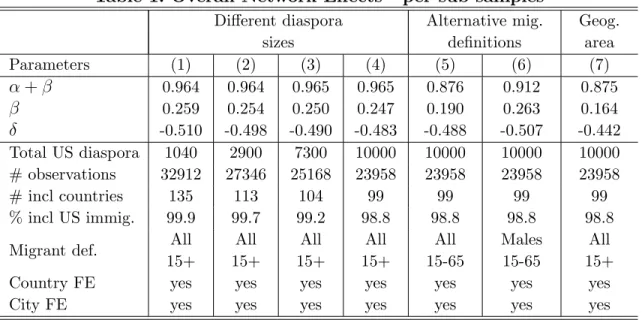
cities is not properly captured in the census data. Following Card (2009), we adjust the initial sample and leave out micro states which we de…ne in terms of the total size of their diaspora in the US. We use di¤erent threshold values of this criterion : 1040, 2900, 7300 and 10000 migrants in the US which correspond to 135, 113, 104 and 99 source countries, respectively. These samples account between 98.8 and 99.9 percent of all migrants and the respective results are reported in columns (1)-(4) of Table 1. The estimate of the national diaspora e¤ect is in line with previous results, such as in Beine et al. (2010). The key parameters are quite stable across subsamples which is mainly due to the fact that we capture almost all of the migrants in the US, although we leave out a number of origin countries. We …nd that a one percent increase in the initial stock of diaspora leads to approximately one percent increase in the bilateral migration ‡ow over a period between 1990 and 2000, given by the coe¢ cient of + . The results further suggest that the diaspora e¤ect is composed of about one fourth by the national policy e¤ect ( ₊ ) and the rest by the local assimilation e¤ect ( ₊ ). Our implied multiplier associated with the policy e¤ect is in line with the one obtained by Jasso and Rozenzweig (1986). Finally, the e¤ect of the distance is also quite consistent with a coe¢ cient of around -0.5, regardless of the sample size.

All of the results in columns (1)-(4) were based on the ‡ows of migrants aged over 15 at time of arrival, regardless of current or arrival age. Next, we use alternative de…nitions of migration ‡ows and show that our estimates are roughly similar. In column (5), the migrants are aged between 15 and 65 at time of arrival and are in the US as of 2000, so it excludes elderly immigrants. In column (6), we take only male migrants aged between 15 and 65 at the time of their arrival between 1990 and 2000. In both of these cases, the results are fairly robust to the choice of alternative measures of the migration ‡ows. The main di¤erence is that the national policy e¤ect is found to be slightly higher for men, indicating the local assimilation e¤ect might in‡uences male migration less strongly when compared to women.

Our identi…cation strategy rests on the de…nition of metropolitan areas by the US Census bureau which de…nes the location of our local network/diaspora. In other words, we assume the migrant and his local diaspora network are located within the same US metropolitan area. In order to test the robustness of this particular assumption, we modify the de…nition of the geographic area corresponding to the local network.We consider that the Mij variable is composed by the number of migrants

from country i living in metropolitan area j as well as in neighboring metropolitan areas that are located within 100 miles from the center of j.8 In general, in about 50 percent of the cases, this leads to an increase in the size of the network. Column (7) provides the estimation results of this change in the geographic area de…nition. We …nd that both e¤ects are roughly similar with the estimates of the comparable regression, presented in column (4). The assimilation/network e¤ect is relatively

8_{When we modify M}

ij , we end up naturally modifying ij in (5) as well. More speci…cally an

stronger and but the policy e¤ect is somewhat lower than in the benchmark regression.

Table 1. Overall Network E¤ects - per sub-samples

Di¤erent diaspora sizes Alternative mig. de…nitions Geog. area Parameters (1) (2) (3) (4) (5) (6) (7) + 0.964 0.964 0.965 0.965 0.876 0.912 0.875 0.259 0.254 0.250 0.247 0.190 0.263 0.164 -0.510 -0.498 -0.490 -0.483 -0.488 -0.507 -0.442 Total US diaspora 1040 2900 7300 10000 10000 10000 10000 # observations 32912 27346 25168 23958 23958 23958 23958 # incl countries 135 113 104 99 99 99 99 % incl US immig. 99.9 99.7 99.2 98.8 98.8 98.8 98.8 Migrant def. All

15+ All 15+ All 15+ All 15+ All 15-65 Males 15-65 All 15+ Country FE yes yes yes yes yes yes yes City FE yes yes yes yes yes yes yes

Notes: ML Poisson estimates of equation (1). All parameters signi…cant at the 1 percent level; otherwise mentioned; robust estimates; Estimation carried out on migrants aged 15 and over, on the 1990-2000 period; threshold in terms of the size of the total diaspora at destination (across all U.S. metropolitan areas).

4.2

Education level

The strength of the diaspora e¤ect tends to decline with the education and the skill levels of the migration ‡ows. The main reason is that unskilled migrants face higher assimilation costs and policy restrictions. Hence they rely more on the diasporas to overcome these barriers. Among recent papers in the literature, McKenzie and Rapoport (2010) use individual data from Mexico and Beine et.al (2010) use bilateral data at the country level to con…rm these patterns.

In line with the existing literature, we di¤erentiate between migrant ‡ows based on their education levels to identify di¤erent skill categories. There is a certain level of imperfection in the census data since the education level is given by the number of years of completed education as reported by the migrants who come from di¤erent countries with di¤erent education regimes. Comparison across origin countries is di¢ cult, but, we aggregate these into three di¤erent categories as is usually done in the literature (Docquier et al., 2009). These categories are (i) low skilled migrants with less than 11 schooling years; (ii) medium skilled migrants with more than 11 schooling years up to high school degree; (iii) the high skilled migrants who have some college degree or more.

We estimate (5) for these three education levels separately and the results are presented in Columns (1)-(3) of Table 2. We speci…cally focus on the migrants who

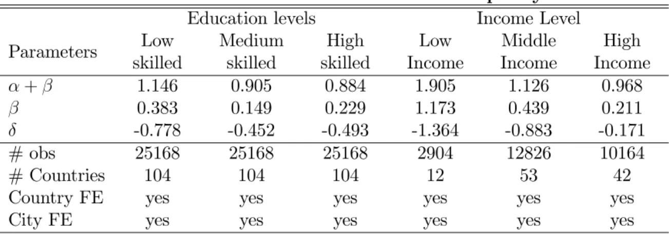
completed their education prior to migration and did not receive any further education in the United States in order to separate out migrants who entered as children with their families and who entered for education purposes o special student visas. In line with previous results, we …nd that the total diaspora e¤ect ( + ) decreases with the education level of migrants, from 1.146 for low skilled to 0.884 for high skilled migrants. Comparing skilled and unskilled migrants, we …nd the local assimilation e¤ect, given by , is higher for low skilled migrants relative to high skilled migrants - at 0.763 vs. 0.655. The di¤erence in the policy e¤ect of the diaspora is, however, much more signi…cant - 0.383 vs. 0.229. These results indicate that the diasporas are more important for the low skilled migrants but the e¤ect is even stronger in overcoming national policy barriers in both relative and absolute terms.

The education distinctions we used above do not fully take into account the het-erogeneity in the quality of education across origin countries. Migrants from di¤erent countries will nominally have the same education levels but a university diploma ob-tained in Canada would, on average, imply higher human capital level than a diploma obtained in a poorer developing country. Educational quality di¤erences might be especially severe since the results are only for migrants who have completed their education at home.

In an innovative paper, using some measures of the observed skills for immigrants in Canada that obtained their education at home, Coulombe and Tremblay (2009) are able to estimate some skill-schooling gap. This approach provides some measure of the quality relative to the national education quality in Canada. They show that the average gap with Canada can amount to more than 4 years of education for some countries.9 _{If the quality of education di¤ers among migrants with the same nominal}

education levels, the ability to migrate outside family reuni…cation programs or other legal channels might be low. In that case, one could expect the national visa and the local assimilation e¤ects to be higher.

There is no common measure of quality of education by origin country. Never-theless, Coulombe and Tremblay (2009) show that the skill-schooling gap is highly correlated with the level of GDP per head in the origin country. In line with this approach, we estimate (5) following the World Bank income classi…cation while con-tinuing to use the thresholds in terms of size of the US diaspora. These groups are (i) low income countries, (ii) middle income countries and (iii) high income countries. Income levels of the origin countries of course capture many e¤ects in addition to the quality of education, such as the level of development of …nancial markets, ability to …nance migration expenses, domestic political conditions, quality of eco-nomic institutions and various other push factors. Results of this estimation exercise are reported in Columns (4)-(6) of Table 2. We …nd that the overall diaspora e¤ect

9_{See also Mattoo, Neagu and Ozden’s (2008) exploration of the brain waste e¤ect where migrants}

with seemingly similar education levels but from di¤erent countries end up at jobs with varying levels of quality in terms of human capital requirements. They conclude that di¤erences in educational quality in the origin country and selection e¤ects explain a large portion of these di¤erences.

decreases with income level from 1.905 for low income countries to 0.968 for high income countries. In line with the previous estimates of columns (1)-(3), we …nd that most of the variation is driven by the national visa/policy e¤ects. The e¤ect of the diaspora size through the visa e¤ect for high-income countries is a minuscule 0.211. On the other hand, it is 0.439 for middle income and 1.173 for low income countries. These results show clearly that the diaspora plays an important role in providing migrants from low income countries legal access to the US. On the other hand, the assimilation e¤ect shows almost no variation - it is 0.732 for low income countries and 0.757 for high income countries. Finally, low-skill migrants are much more sensitive to distance as seen with the sharp decline in the coe¢ cient of distance with income levels.

Table 2. Results - Education level and quality

Education levels Income Level Parameters Low skilled Medium skilled High skilled Low Income Middle Income High Income + 1.146 0.905 0.884 1.905 1.126 0.968 0.383 0.149 0.229 1.173 0.439 0.211 -0.778 -0.452 -0.493 -1.364 -0.883 -0.171 # obs 25168 25168 25168 2904 12826 10164 # Countries 104 104 104 12 53 42

Country FE yes yes yes yes yes yes

City FE yes yes yes yes yes yes

Notes: ML Poisson estimates of (5) on countries with less than 7300 migrants. All parameters signi…cant at the 1 percent level, otherwise mentioned; robust estimates.

4.3

Distance thresholds

Distance plays a key role in migration patterns as an important barrier. Furthermore, it has a di¤erent impact on migrants with varying skill levels and, as a result, op-erates as a selection mechanism. This di¤erential impact is re‡ected in the distance coe¢ cients in the earlier estimations in Table 2. Even though we have country …xed e¤ects which may control for bilateral distances in many gravity estimations, due to the sheer size of the United States, there is still signi…cant variation in terms of the distance and accessibility from origin countries to di¤erent American cities. For in-stance, the Caribbean and Central American countries that are close to the US, will send more migrants to cities in the south compared to the north. In the subsequent estimations, we de…ne far and close countries on the basis of the minimal distance to the US border with a cuto¤ of 6790 kilometers which is the median distance in terms of pairs of origin countries and US metropolitan areas. We also consider the e¤ect of distance for di¤erent education levels - low and high skilled.

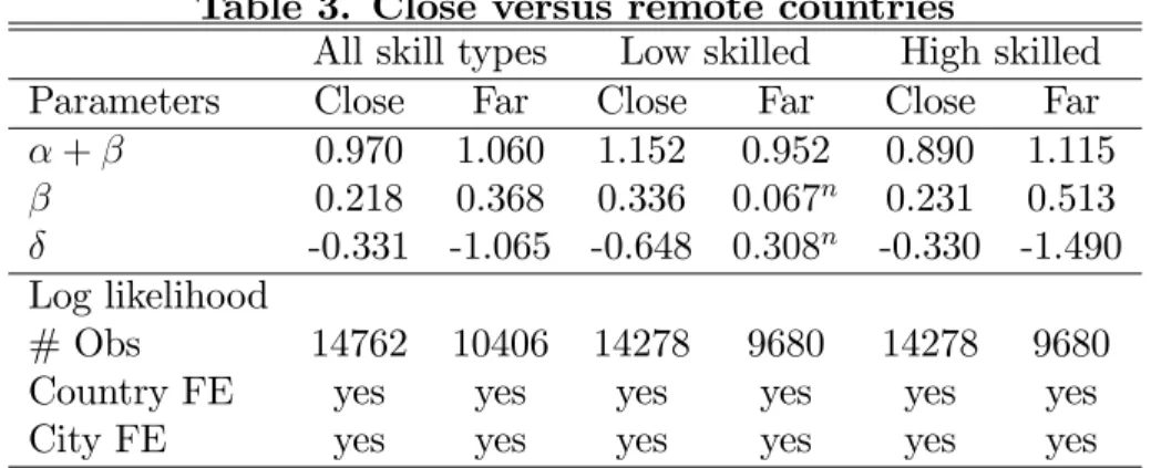
First, we …nd that distance plays a much more important role for migrants com-ing from far away countries. The coe¢ cient of the distance variable is signi…cantly lower in absolute value when the origin countries are closer to the US and these tend to be Latin American and Caribbean countries. Second, the overall diaspora e¤ect is slightly higher when origin countries are far away but this is not statistically sig-ni…cant. However, there is a di¤erence in terms of the composition. The national policy e¤ect is higher for far away countries while the local assimilation e¤ect is more important for closer countries.

Table 3. Close versus remote countries

All skill types Low skilled High skilled Parameters Close Far Close Far Close Far

+ 0.970 1.060 1.152 0.952 0.890 1.115 0.218 0.368 0.336 0:067n _{0.231 0.513}

-0.331 -1.065 -0.648 0:308n -0.330 -1.490 Log likelihood

# Obs 14762 10406 14278 9680 14278 9680 Country FE yes yes yes yes yes yes City FE yes yes yes yes yes yes

Notes: ML Poisson estimates of (5) on the ‡ow of migrants aged 15 and over from countries with more than 10,000 migrants in the US.All parameters signi…cant at the 1 percent level, except those superscripted n (non signi…cant). If not mentioned, robust estimates. Cut o¤ value to de…ne far and close: 6790 kilometers.

We obtain more nuanced results when we compare the importance of distance for di¤erent education levels. For unskilled migrants, distance seems to be a very signi…cant deterrent to the extent that it becomes prohibitive. We …nd that for the unskilled migrants from distant countries, the policy e¤ect is almost non-existing. On the other hand, for skilled migrants from far away countries, the visa e¤ect is much stronger when compared to nearby countries. Finally, we see that the di¤erence in the local assimilation e¤ect between distant and nearby countries becomes small when we control for the skill level. The earlier di¤erence in Columns (1)-(2) is simply due to the skill composition of migrants. In other words, once the migrants pass the border and enter the US, the local assimilation e¤ect of the diaspora does not di¤er based on the country of origin.

4.4

Dropping small cities

In order to assess the robustness of our results, it might also be desirable to measure to what extent our …ndings are driven by the inclusion of small citieswhich we de…ne as metropolitan areas with a low number of migrants. One of the reasons of that concern is that small cities exhibit a lot of zero values at the dyadic level forln(1 +Mij) and

ln(1 + ij), leading in turn to spurious correlation between the two variables. To

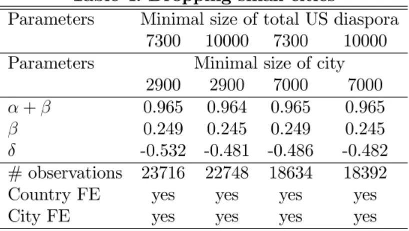
that sake, we reestimate equation (5), dropping small countries and small cities. As before, we drop countries with less than 7300 or 10000 migrants in the US. Further, we also drop small cities having less than 2900 migrants or less than 7000 migrants. Combining the two cut-o¤ values yields four alternative regressions which are reported in Table 4. The results are highly robust to the exclusion of small cities. The value of the assimilation and of the policy e¤ect are hardly a¤ected by the exclusion of small countries and small cities.

Table 4. Dropping small cities

Parameters Minimal size of total US diaspora 7300 10000 7300 10000 Parameters Minimal size of city

2900 2900 7000 7000

+ 0.965 0.964 0.965 0.965 0.249 0.245 0.249 0.245 -0.532 -0.481 -0.486 -0.482 # observations 23716 22748 18634 18392 Country FE yes yes yes yes City FE yes yes yes yes

Notes: Poisson estimates. All parameters signi…cant at the 1 percent level; otherwise mentioned; robust estimates; Estimation carried out on migrants aged 15 and over, on the 1990-2000 period; threshold in terms of the size of the total diaspora at destination (across all U.S. metropolitan areas).

4.5

Flows in the 90’s vs 80’s

Our analysis in the previous sections focused on the e¤ect of the 1990’s diaspora level on the migration ‡ows between 1990 and 2000. Our dataset includes parallel measures for the migration patterns in the 1980’s. It is useful to perform the same estimation on the ‡ows observed in the 1980’s to observe if there has been any important changes in the patterns and the relative e¤ects. One possibility is to combine observations from the 1980’s with those from the 1990’s and adopt a panel approach by pooling the data from the two cross section. Nevertheless, it is very likely that the expected e¤ects ( and ) will be di¤erent over time and prevent us from pooling our data across time.

While it is unclear if there has been any signi…cant cultural shift in the US to change the assimilation e¤ect ( ), the US immigration policy has experienced several modi…cations between the 1980s and the 1990s. The main change is the strengthen-ing of the family reuni…cation between the 1980’s and the 1990’s with the 1990 US immigration act which clearly expanded opportunities for family reuni…cation. This leads to two additional aspects that are not directly modi…ed with the 1990 law but

exert important e¤ect on the extent of family reuni…cation in the aftermath. The …rst feature is that the immediate relatives of US citizens are not limited or capped under the law. Therefore, quotas for family reuni…cation that are established in the law can be exceeded in practice if the applications by immediate family members are above the estimated number by the law for a given year. As a result, as more immigrants obtain US citizenship, there is a natural upward trend in the number of people coming under the family reuni…cation scheme sensu lato. The second impor-tant feature is related to the amnesty or legalization programs undertaken in 1986 via the Immigration Reform and Control Act. As large numbers of undocumented migrants obtain legal resident status, they become eligible to bring additional family members through the legal channels. Those who became citizens were even able to bring their relatives through the uncapped channel. Therefore, these policy devel-opments suggest that the estimated coe¢ cient should have increased between the 1980’s and 1990’s.

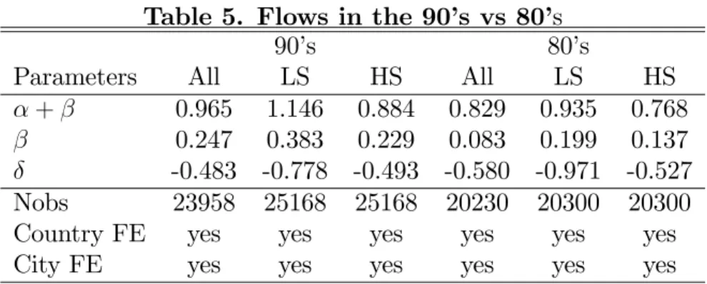
Table 5. Flows in the 90’s vs 80’s

90’s 80’s

Parameters All LS HS All LS HS

+ 0.965 1.146 0.884 0.829 0.935 0.768 0.247 0.383 0.229 0.083 0.199 0.137 -0.483 -0.778 -0.493 -0.580 -0.971 -0.527 Nobs 23958 25168 25168 20230 20300 20300 Country FE yes yes yes yes yes yes City FE yes yes yes yes yes yes

Notes: All = All skill types; LS = low skilled; HS = high skilled. ML Poisson estimates of (5) on countries with more than 7300 migrants. All parameters signi…cant at the 1 percent level ; robust estimates. Estimation carried out on migration ‡ows of individuals aged 15 and over.

Table 5 reports the estimates obtained for the 1990’s and the 1980’s. For each period, we consider three alternative types of migrants: those with low education level, those with high education and all migrants. Our estimates suggest that the family reuni…cation e¤ects are uniformly stronger for the 1990’s than for the 1980’s for all immigrant categories. Naturally, the change is more important for unskilled migrants, more than doubling within a decade. This is in line with the impacts associated with the legalization programs which primarily e¤ect undocumented migrants. In short, the comparison between the 1980’s and the 1990’s shows that our estimation of the policy e¤ect is in line with what is expected from the evolution of the US immigration policy. On the other hand, the coe¢ cient of stays around 0.75 for low skilled and 0.65 for high-skilled migrants across both decades, indicating the local assimilation e¤ect did not change considerably.

4.6

Additional econometric issues.

Our benchmark regression model involves a stock-‡ow relationship. Since immigrant stocks at the beginning of the period includes past migration ‡ows, the current model could also be written as an autoregressive model involving current and past migration stocks. In such a framework, the network e¤ect can be recovered from the estimated autoregressive coe¢ cient. In panel data and cross section framework, the estimation of autoregressive model is nevertheless subject to some bias, known as the Nickell bias (Nickell, 1981). Furthermore, the bias is supposed to be serious for panel data with few periods, like in our case.

A traditional approach to take care of the Nickell bias is to use instrumental vari-ables to predict value ofMij using a variable that is uncorrelated withNij. Tenreyro

(2007) proposes a method to combine Poisson estimators with instrumental variables estimator which can be done in the GMM context. Dropping thes subscript for con-venience of exposition and aggregating all explanatory variables cs

j, msi, dij and Mij

into the xij vector, the Poisson estimator solves the following moment condition: n

X

ij

[Nij exp(xij )]xij = 0: (7)

In order to instrumentxij, one can use as an alternative the following GMM estimator

denoted by :

n

X

ij

[Nij exp(xij )]zij = 0 (8)

in whichzij represent the vector of instruments, i.e. variables that are supposed to be

correlated withMij but uncorrelated withNij. In this robustness analysis, we rely on

the GMM estimator using two potential instruments. Those instruments are the variablesln(1 +Mij)and ln(1 + ij) observed in 1950, i.e. about 40 years before the

observed diaspora in the benchmark regression. Those variables are well correlated with their values in 1990 (part of the stock of 1990 was already present in 1950). In contrast, the network and policy e¤ects on the ‡ows during the 1990’s associated to migrants already present in 1950 are supposed to be quite limited. One drawback of using such an instrument is that it leads to a change in the available sample. This is …rst due to the fact that the de…nition of origin countries and US metropolitan areas has signi…cantly changed between 1950 and 1990. A second reason is the independence of many former colonies during the 50’s and 60’s.10 _{Therefore, in the robustness}

analysis, we show on comparable samples that our benchmark regressions relying on Poisson regressions are not a¤ected by the potential correlation betweenMij and sij.

In other terms, we show that the estimates for and for are quite close on identical samples.

10_{For instance, all US migrants coming from former European colonies were identi…ed as migrants}

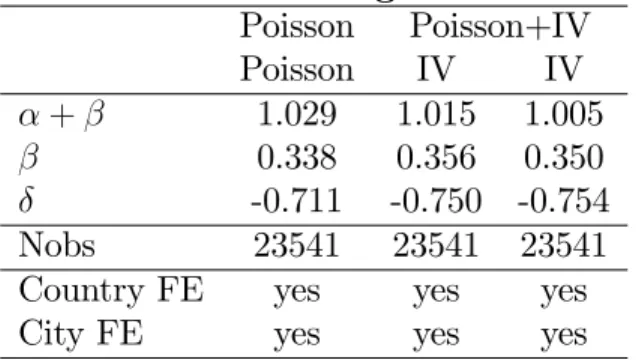
In practice, we …rst reestimate the Poisson regressions and use those estimates as a benchmark with respect to the ’IV’(GMM) estimates. Table 6 report the estimates of the Poisson on the restricted sample (column 2) and of the combined Poisson and IV estimatesà la Tenreyro in column 3 and 4. In column 3 we use one instrument only, i.e. ln(1 +Mij) observed in 1950 while in column 4 we supplement the instrument

set withln(1 + ij)observed in 1950, too.11

The results show that our estimates are strikingly robust to the instrumentation procedure. Both the total diaspora e¤ect and the estimated policy e¤ect are very sim-ilar across estimation methods. They are also very simsim-ilar regardless of the inclusion or not of ln(1 + ij) variable observed in 1950.

Table 6. Instrumenting network sizes

Poisson Poisson+IV Poisson IV IV + 1.029 1.015 1.005 0.338 0.356 0.350 -0.711 -0.750 -0.754 Nobs 23541 23541 23541 Country FE yes yes yes City FE yes yes yes

Notes: First column : ML Poisson estimates of (5). Two last columns: GMM estimates. All parameters signi…cant at the 1 percent level ; robust estimates. Estimation carried out on migration ‡ows of individuals aged 15 and over. Instrument for IV estimates in col 3 : local network size observed in 1950. Instruments for IV estimates in col 4: local and national network sizes observed in 1950.

Another potential econometric issue is generated by the presence of unobserved bilateral factors s

ij in‡uencing the bilateral migration ‡ows Nijs. In absence of

ob-servations for those factors, their e¤ect will be included in the composite error term given by sij +usij = sij.12 If those factors also in‡uence the diaspora Mij, this leads

to some correlation between the error term and one covariate, invalidating the use of OLS (and Poisson) estimators. This is known as the re‡ection problem (Mansky,

11_{Note that , we checked the robustness of the maximum likelihood estimator. Indeed, the use of}

the Pseudo Poisson Maximum Likelihood might lead to convergence problems and might generate spurious convergence. Following Santos Silva and Tenreyro (2010), the issue might be addressed through some iterative procedure dropping the insigni…cant country and city …xed e¤ects.

12_{Note that the non observation of} s

ij is also due to the fact that our data is of cross sectional

nature. In fact, if one could introduce the time dimension in (5), one could estimate s_ij through bilateral …xed e¤ects. In our case, the use of time through a panel data framework is not possible because of the clear rejection of the pooling assumption. In fact, it is obvious that some parameters such as the one capturing the visa e¤ect ( s) are not constant over time. In the robustness analysis, we document the change in the US migration policy and show that the sparameter changes between the 1980’s and the 1990’s.

1993). Once again, the solution to that issue is to use instrumental variable, with instruments uncorrelated with Ns

ij and sij, but correlated with Mijs

The key question is whether the unobservable components are highly persistent over time (more than 50 years). If it is the case, our instrument (correspond variables in 1950) is likely to be correlated with s

ij, invalidating the exclusion condition. For

instance, one often quoted unobserved factor involves climate variables such as aver-age temperature of averaver-age rain falls in the sense that they will a¤ect the choice of migrants coming from some countries. It is claimed that contemporaneous migrants (i.e. theNs

ij variable) and the previous ones (i.e. theMij variable) follow the same

cli-matic pattern. Nevertheless, our data show that it is not the case. Mexican migrants in the 1950’s had obviously a strong preference for nearby metropolitan areas with similar climatic conditions. This is obviously not the case anymore since Mexican migrants have spread out all over the US. Another example involves the Porto Rican migrants who tend to concentrate in New York where the climate is quite di¤erent from the one prevailing in Porto Rico.

To sum up, our IV procedure takes care of the re‡ection problem to the extent that the factors not included in the regression (either because that are omitted or because they are unobservable) are not highly persistent over time, i.e. over a period of 50 years.

4.7

In‡uence of the homogeneity assumption

Our identi…cation strategy assumes that the functional form for the local assimila-tion and the visa externalities of the diaspora network are identical. In particular, we assume that both externalities are log-linear. It might also be desirable to as-sess whether this homogeneity assumption a¤ects our results. One possibility is to estimate directly and in equation (4). Unfortunately, this is not possible if one accounts for unobserved heterogeneity across origin countries via inclusion of the s i

in the estimated equation. As an alternative, we can proceed to a two-step estima-tion of equaestima-tion (4). In the …rst step, we estimate the following equaestima-tion via Poisson maximum likleliood estimation:

lnN_ijs = s_i + s_j slndij + sln (1 +Mij) + ij (9)

where ij is an error term. This …rst estimation yields the coe¢ cient for for the

1990’s. Interestingly, using a cut-o¤ value of 7300 US migrants to exclude small countries, we get an estimated value for the coe¢ cient of equal to 0.719. This is strikingly close the implied value of in Table 1, i.e. 0.714. Then, in order to recover the coe¢ cient of si, we can estimate the value of with the following country-level

regression :

i = + ln(1 +Mi) + 0Xik+!i (10)

where !i is an error term and where Xik are country-speci…c time-invariant factors

Xik is supposed to account for the variability in the i that is unrelated to the policy

e¤ect. We consider four potential factors : trade openness captured by the share of export to gdp, gdp per head in 1990, a dummy variable capturing whether the country speaks English of not and a regional dummy as de…ned by the World Bank o¢ cial classi…cation. In line with section 4.3., the sign of the GDP/head variable should be expected to be negative as rich countries are shown to have a lower value for the policy e¤ect. The estimation tends to con…rm this expectation.

The following exercise should be nevertheless seen as a sub-optimal procedure, aimed only at guessing the importance of the linearity assumption for both external-ities. The reason is two-fold. First, the method is a two-step method, which is less e¢ cient that the one step estimation methods like the one used before. Second, the inclusion of observable variables and the estimation of country …xed e¤ects lead to small sample sizes.

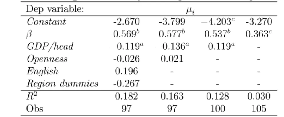
Table 10 reports the estimation results. The results suggest that the impact of economic development is negative, as expected. The estimated value of ranges between 0.36 and 0.57. This is slightly higher than in Table 1, leading to policy e¤ect representing about 40% of the total network e¤ect instead of the previously obtained 25%. Nevertheless, given that the procedure is quite di¤erent, the results are relatively similar and this robustness check procedure con…rms that the local assimilation e¤ect tends to dominate the global policy e¤ect of the diaspora network. All in all, this exercise suggests that our identi…cation strategy yields results that make sense, but that the linearity assumption might lead to a small underestimation of the value and the share of the policy e¤ect.

Table 7. Assessing the linearity assumption: two-step estimation

Dep variable: _i Constant -2.670 -3.799 4:203c -3.270 0:569b _0:577b _0:537b _0:363c GDP/head 0:119a _0:136a _0:119a -Openness -0.026 0.021 - -English 0.196 - - -Region dummies -0.267 - - -R2 _{0.182 0.163 0.128 0.030} Obs 97 97 100 105

Notes: First step estimation : see equation (4). Cut-o¤ values of inclusion of origin countries: 7300 migrants. Second step estimated equation : _i = + ln(1 +Mi) + Xi+ui.

Note that the …rst step estimated is 0.719. a, b, c: signi…cant at 1%, 5% and 10% level respectively.

5

Conclusion

This paper deals with the network e¤ect in international migration. In particular, it proposes a new approach aimed at disentangling the two main components of the network e¤ect, i.e. the assimilation e¤ect and the policy e¤ect. Using migration data at the city level and at the country level, we are able to isolate the policy e¤ect from the global network e¤ect for the US.

We show that for the US, the average network elasticity is close to unity, with 25 % of it associated to the policy e¤ect and 75% of it associated to the assimila-tion e¤ect. This baseline result is in line with the existing literature (Jasso et al., 1986, 1989) suggesting that the medium-run migration multiplier associated to family reuni…cation lies around 1.3.

Furthermore, we …nd that the size and the composition of the network e¤ect vary across a set of characteristics of the migrants. The policy e¤ect is larger for unskilled migrants and those coming from low income countries. Furthermore, the policy e¤ect has signi…cantly increased between the 80’s and the 90’s, re‡ecting a higher share of kinship based migration in the US, favored either by changes in the immigration laws or by other policies such as the legalization programs.

6

References

Bauer, Thomas, Gil Epstein, Ira N. Gang (2007). Herd E¤ects or Migration Net-works? The Location Choice of Mexican Immigrants in the U.S. Research in Labor Economics 26, 199-229.

Beine, Michel, Frédéric Docquier, Caglar Ozden (2010). Diasporas. Journal of Development Economics, forthcoming.

Bin, Yu (2007). Chain Migration Explained: The Power of the Immigration Multiplier. LBF Scholar Publishing: El Paso, U.S.

Boyd, Monica (1989). Family and Personal Networks in International Migration: Recent Developments and New Agendas. International Migration Review 23 (3), 638-670.

Card, David (2009), Immigration and Inequality, NBER Working Paper 14683. Coulombe, Serge, Jean-Francois Tremblay (2009), Migration and Skill Disparities Across the Canadian Provinces, Regional Studies 43 (1), 5-18.

de Meza, David (1987). The Migration Multiplier. Bulletin of Economic Research 39 (3), 243-48.

Epstein, Gil (2008). Herd and network e¤ects in migration decision-making. Jour-nal of Ethnic and Migration Studies 34 (4), 567-583.

Gang, Ira N. and Luis A. Rivera-Batiz (1994). Labor Market E¤ects of Immigra-tion in the United States and Europe: SubstituImmigra-tion vs. Complementarity. Journal of Population Economics 7, 157-175.

Grogger, Je¤rey, Hanson, Gordon H. (2010). Income Maximization and the Sort-ing of Emigrants across Destinations, Journal of Development Economics, forthcom-ing.

Jasso, Guillermina, Mark R. Rosenzweig (1986).Family reunion and the immigra-tion multiplier: U.S. immigraimmigra-tion law, origin-country condiimmigra-tions, and the reproduc-tion of immigrants. Demography 23 (3), 291-311.

Jasso, Guillermina, Mark R. Rosenzweig (1989). Sponsors, Sponsorship Rates and the Immigration Multiplier. International Migration Review 23 (4), 856-888.

Manski, Charles F. (1993). Identi…cation of Endogeneous Social E¤ects: the Relection Problem. Review of Economic Studies 60 (3), 531-42.

Massey, Douglas, Joaquim Arango, Graeme Hugo, Ali Kouaouci, Adela Pelle-grino and J. Edward Taylor (1993). Theories of international migration: Review and Appraisal.”Population and Development Review 19 (3), 431-466.

Matoo, Aaditya, Ileana Cristina Neagu and Caglar Ozden (2008), Brain Waste? Educated Immigrants in the U.S. Labor Market, Journal of Development Economics 87(2), 255-269.

McFadden, DanielL. (1984). Econometric analysis of qualitative response models. In: Z. Griliches and M. Intriligator, eds., Handbook of Econometrics, Volume 2, Amsterdam. Elsevier/North-Holland.

McKenzie, David, Hillel Rapoport (2010). Self-selection patterns in Mexico-US migration: the role of migration networks. Review of Economics and Statistics, forthcoming.

Munshi, Kaivan (2003).“Networks in the modern economy: Mexican migrants in the US labor market. Quarterly Journal of Economics 118 (2), 549-99.

Nickell, Stephen (1981), Biases in dynamic models with …xed e¤ects. Economet-rica 49, 1417–1426.

Pedersen, Peder J., Mariola Pytlikova , Nina Smith (2008). Selection or Network E¤ects? Migration Flows into 27 OECD Countries, 1990-2000. European Economic Review 52 (7), 1160-1186.

Piacentini, Mario (2010). Enclaves and schooling choices of young migrants. Mimeo-graph: University of Geneva.

Santos Silva, J.M.C. and S. Tenreyro (2006), The Log of Gravity, Review of Economics and Statistics 88 (4), 641-658.

Santos Silva, J.M.C and Tenreyro, S. (2010), On the Existence of the Maximum Likelihood Estimates for Poisson Regression, forthcoming in Economic Letters.

Tenreyro, S. (2007), On the Trade Impact of Nominal Exchange Rate Volatility, Journal of Development Economics 82 (2), 485-508.

Winters, Paul, Alain de Janvry, Elisabeth Sadoulet (2001). Family and Com-munity Networks in Mexico-U.S. Migration. Journal of Human Resources 36 (1), 159-184.