AT2 PROBLEM SET #3
Problem 1
We want to simulate a neuron with autapse. To make this we use Euler method and we simulated system for different initial values.
(a) Neuron’s activation function
from pylab import * from numpy import * from math import * import os
if not os.path.exists(__file__[:-3]): #create a directory with the name of file to put the pictures
os.makedirs(__file__[:-3])
f = [50*(1 + tanh(x)) for x in linspace(-5,5,1000)] # list of f for s in [-5,5]
plot(linspace(-5,5,1000),f) # print the curve
titre = 'Neuron\'s activation function'
title(titre)
ylabel('Firing rate [Hz]')
xlabel('Current [nA]')
savefig(__file__[:-3] + '/' + titre + '.png')
We can see that activation of neuron increase with the current which is inject in it. But augmentation is not linear. For weak input (less than -3nA), the neuron doesn’t create spiking. Then, the firing rate is increasing more rapidly with a highest augmentation of firing rate for current (the curve look like the hyperbolic tangent that we use to create the dynamic of neuron). We observe finally a saturation: for current upper than 3nA, the maximum firing rate is 100 Hz.
(b) Plot of dx/dt from pylab import * from numpy import * from math import * import os
if not os.path.exists(__file__[:-3]): #create a directory with the name of file to put the pictures
os.makedirs(__file__[:-3])
w = 0.04 # strength of the synaptic connection
I = -2 #nA # input
list = linspace(0,120,10000) # differents values of firing rate x
def f(x): # value of the sigmoidal function
dx = [-x + f(w*x+I) for x in list] # list of dx with the list values
plot(list,dx)
titre = 'dx in function of the neuron\'s firing rate'
title(titre)
ylabel('Devivate')
xlabel('Firing rate [Hz]')
savefig(__file__[:-3] + '/' + titre + '.png')
close()
On this plot, the zero-crossings indicate that the derivate of x, dt, is null. So it’s a fixe point of the dynamic system because x+dt = x.
(c) Simulation of system from pylab import * from numpy import * from math import * import os
if not os.path.exists(__file__[:-3]): #create a directory with the name of file to put the pictures
os.makedirs(__file__[:-3])
w = 0.04 # strength of the synaptic connection
dt = 0.01 # ms # time steps
sim_time = 50 #simulation time
def f(x): # value of the sigmoidal function
return 50*(1 + tanh(x))
for x0 in [49,50,51]: # we make simulation for differents x0
x = [] # we initialize
x.append(x0)
dx = []
dx.append(0)
for i in arange(dt,sim_time,dt): # we make simulation
x.append(x[-1] + (-x[-1] + f(w*x[-1]+I))*dt) # we use euler method
dx.append(dt*(-x[-1] + f(w*x[-1]+I))) # we capture dx to plot orbite
plot(arange(0,sim_time,dt),x)
titre = 'Simulation of x over time for x0 = ' + str(x0)
title(titre)
ylabel('Firing rate [Hz]')
xlabel('Time [s]')
savefig(__file__[:-3] + '/' + titre + '.png')
close()
plot(x,dx,'o')
titre = 'Trajectory of x for x0 = ' + str(x0)
title(titre)
ylabel('X\'')
xlabel('X')
savefig(__file__[:-3] + '/' + titre + '.png')
close()
We simulate the system for three initial conditions: - x(0) = 49
Here we see that 49 is not a fixe point. The trajectory is repulse by 50 and come to the fixe point near to zero. We see on the orbite that dx is decrease more and more rapidly when the point is next to 50. Then,
when it is next to zero, the convergence speed is slower. The speed of convergence have a pic next to 30. This particular change of velocity is due to the hyperbolic tangent function in the dt calcul.
- x(0) = 50
Here 50 is a fix point. So the firing rate stay the same all long the simulation. There is no evolution of orbite in the trajectory plan.
- x(0) = 51
When initial condition is 51Hz, firing rate change to the fix point near to 100Hz. Like for x(0) = 49, velocity is increasing and decreasing during the trajectory, due to hyperbolic tangent function.
(d) Noise in the system! from pylab import * from numpy import * from math import * import os
if not os.path.exists(__file__[:-3]): #create a directory with the name of file to put the pictures
os.makedirs(__file__[:-3]) import random
w = 0.04 # strength of the synaptic connection
I = -2 # input
dt = 0.01 # time steps
sim_time = 50 #simulation time
def f(x): # value of the sigmoidal function
return 50*(1 + tanh(x))
for sigma in [5, 80]: #sigma value for the noise
for x0 in [49,50,51]: # we make simulation for differents x0
x = [] # we initialize
x.append(x0)
for i in arange(dt,sim_time,dt): # we make simulation
x.append(x[-1] + (-x[-1] + f(w*x[-1]+I) + sigma *
random.gauss(0,1))*dt) # we use euler method and put the noise term with sigma times a gaussian aleatory value
plot(arange(0,sim_time,dt),x)
titre = 'Simulation of x over time for x0 = ' + str(x0) + '
with noise sigma = ' +str (sigma)
title(titre)
ylabel('Firing rate [Hz]')
xlabel('Time [s]')
savefig(__file__[:-3] + '/' + titre + '.png')
close()
Sigma = 5 Sigma = 80
50
51
For a noise with a weak sigma, variance is small so we have the same curves that question c, with little variation due to white noise. For variance equal to 80, we have big variation in the signal. The white noise is too strong and the signal seems converge to zero in the three case for this example but they could
converge to 100 Hz too. It’s depend of in which side of 50Hz the signal come to at the beginning (it’s random because of the white noise).
Problem 2
We want to simulate two neurons network. Each neuron inhibited the other and they discharge spontaneously.
(a) Null-clines of system from pylab import * from numpy import * from math import * import os
if not os.path.exists(__file__[:-3]): #create a directory with the name of file to put the pictures
os.makedirs(__file__[:-3]) import random
w = -0.1 # strength of the synaptic connection
I = 5 # nA # input
dt = 0.1 # ms
list = linspace(0.001,99.999,1000) # list of x1 values
def f(x): # value of the sigmoidal function
return 50*(1 + tanh(x))
x = [] # we initialize
for i in list: # we make simulation
x.append(f(w*i+I)) # the nullcline have the same calcul for x1 and x2
# the code below it's to have the direction vectors on the plot
L = 100 Dt = 5 u = [] v = [] for i in range(0,L+1,Dt): u.append([]) v.append([]) for j in range(0,L+1,Dt): u[i/Dt].append((-i + f(w*j+I))*dt) v[i/Dt].append((-j + f(w*i+I))*dt) #
plot(list,x,x,list,list,[50 for i in list],'k--') #
titre = 'Nullclines of the system'
title(titre) ylabel('X2') xlabel('X1') axis([-0.5,100.5,-0.5,100.5]) t= range(0,L+1,Dt) z = range(0,L+1,Dt)
quiver(array(t), array(z), array(v), array(u), angles='xy',
scale_units='xy', scale=1.5)
savefig(__file__[:-3] + '/' + titre + '.png')
It seems that they are three fix point in this system: (0,100), (100,0) and (50,50). We note that the fix point (50,50) is attractive if trajectory is on the diagonal (X1=X2) but repulsive otherwise.
(b) Simulation of system from pylab import * from numpy import * from math import * import os
if not os.path.exists(__file__[:-3]): #create a directory with the name of file to put the pictures
os.makedirs(__file__[:-3]) import random
w = -0.1 # strength of the synaptic connection
list = linspace(0.001,99.999,1000) # list of x1 values
I = 5 # nA # input
dt = 0.1 # ms
time = 10 #time of the simulation
def f(x): # value of the sigmoidal function
return 50*(1 + tanh(x))
x = [] # we initialize
for i in list: # we make simulation
x.append(f(w*i+I)) # the nullcline have the same calcul for x1 and x2
plot(list,x,'y',x,list,'y') #plot of the two null isoclines
list_initial = [(60,80),(99,99),(20,5)]# list of initial values for x1 and x2
for a,b in list_initial:
x = -20*ones(time/dt) # vector of solution
x1_init = a x2_init = b
x[x1_init] = x2_init
for i in arange(dt, time, dt):
x1 = x1_init + (-x1_init + f(w*x2_init+I))*dt #find the next step value of x1
x2 = x2_init + (-x2_init + f(w*x1_init+I))*dt x1_init = x1
x2_init = x2
x[x1_init] = x2_init #append the value of x2 in the x1 emplacment
plot(linspace(0,100,time/dt),x,'o')
# the code below it's to have the direction vectors on the plot
L = 100 Dt = 5 u = [] v = [] for i in range(0,L+1,Dt): u.append([]) v.append([]) for j in range(0,L+1,Dt): u[i/Dt].append((-i + f(w*j+I))*dt) v[i/Dt].append((-j + f(w*i+I))*dt) #
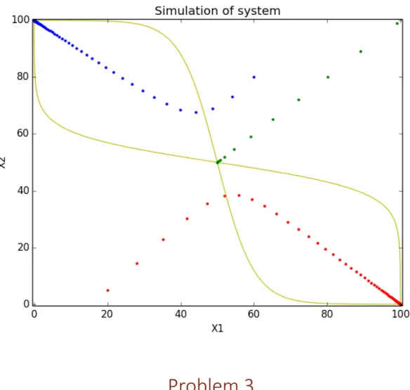
titre = 'Simulation of system'
title(titre) ylabel('X2') xlabel('X1') axis([-0.5,100.5,-0.5,100.5]) t= range(0,L+1,Dt) z = range(0,L+1,Dt)
quiver(array(t), array(z), array(v), array(u), angles='xy',
scale_units='xy', scale=1.5)
savefig(__file__[:-3] + '/' + titre + '.png')
Here the initial conditions are: x(0) = (60,80) (blue), x(0) = (99,99) (green), x(0) = (20,5) (red). We can see that if initial condition are below the diagonal were X1= X2, dynamical system converge to (100,0), this means that neuron X1 firing a lot when X2 stop firing. If initial condition is above diagonal, inverse event occur: X2 firing a lot (100 Hz) and X1 stop firing. Finally, if X1 = X2 at the beginning, system converge to (50,50) : the two neurons firing with the same rate.
(c) Matrix version from pylab import * from numpy import * from math import * import os
if not os.path.exists(__file__[:-3]): #create a directory with the name of file to put the pictures
os.makedirs(__file__[:-3]) import random
w = -0.1 # strength of the synaptic connection
I1 = 5 #nA# input
I2 = 5 #nA
list = linspace(0.001,99.999,1000) # list of x1 values
time = 10 #time of the simulation
def f(x): # value of the sigmoidal function
return array([[50],[50]])*(array([[1],[1]]) +
array([[tanh(x[0][0])],[tanh(x[1][0])]]))
x = [] # initialisation of vector x
W = array([[0,w],[w,0]]) # initialisation of matrix W
I = array([[I1],[I2]]) # initialisation of vector I
for i in list: # we make simulation
x.append(array([[i],f(dot(W,[[i],[i]])+I)[1]])) # we can plot x1 in function of x2 with the inverse function
plot(list,[b[0] for [a,b] in x],'y',[b[0] for [a,b] in x],list,'y') #plot of the two null isoclines
list_initial = [(60,80),(99,99),(20,5)]# list of initial values for x1 and x2
for a,b in list_initial:
x = [] # initialisation of vector x
x.append(array([[a],[b]])) for i in arange(dt, time, dt):
x.append(x[-1] + (-x[-1] + f(dot(W,x[-1])+I))*[[dt],[dt]])
plot([a[0] for [a,b] in x],[b[0] for [a,b] in x],'.')
titre = 'Simulation of system'
title(titre)
ylabel('X2')
xlabel('X1')
axis([-0.5,100.5,-0.5,100.5])
savefig(__file__[:-3] + '/' + titre + '.png')
Problem 3
We construct a Hopfield network in which each neurons is connect with the other (in this case). With this type of network, we can save patterns and system could converge to them.
(a) An example of pattern from pylab import * from numpy import * from math import * import os
if not os.path.exists(__file__[:-3]): #create a directory with the name of file to put the pictures
os.makedirs(__file__[:-3]) import random
fig, ax = plt.subplots()
N = 64
p = array([-1 if random.randint(0,1) == 0 else 1 for i in range (N)])
#create a 64 point vector
p = p.reshape((8,8)) # reshape as a 8*8 matrix
cbar = fig.colorbar(figure, ticks=[-1, 0, 1])
cbar.ax.set_yticklabels(['-1', '0', '1'])# vertically oriented colorbar
titre = 'Pattern matrix'
title(titre)
savefig(__file__[:-3] + '/' + titre + '.png')
close()
A blue square correspond at a -1 weight between two neurons and red correspond to a positive weight. (b) Evolution with one pattern stored in weight matrix
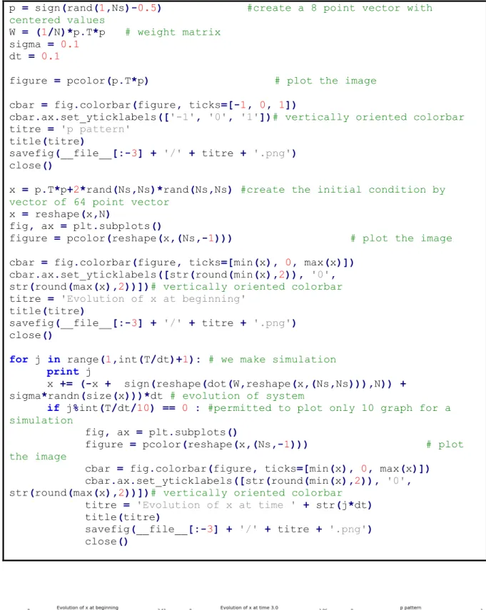
from pylab import * from numpy import * from math import * import os
if not os.path.exists(__file__[:-3]): #create a directory with the name of file to put the pictures
os.makedirs(__file__[:-3]) import random fig, ax = plt.subplots() N = 64.0 Ns = sqrt(N) dt = 0.1 T = 3.0
p = sign(rand(1,Ns)-0.5) #create a 8 point vector with centered values
W = (1/N)*p.T*p # weight matrix
sigma = 0.1
dt = 0.1
figure = pcolor(p.T*p) # plot the image
cbar = fig.colorbar(figure, ticks=[-1, 0, 1])
cbar.ax.set_yticklabels(['-1', '0', '1'])# vertically oriented colorbar
titre = 'p pattern'
title(titre)
savefig(__file__[:-3] + '/' + titre + '.png')
close()
x = p.T*p+2*rand(Ns,Ns)*rand(Ns,Ns) #create the initial condition by vector of 64 point vector
x = reshape(x,N)
fig, ax = plt.subplots()
figure = pcolor(reshape(x,(Ns,-1))) # plot the image
cbar = fig.colorbar(figure, ticks=[min(x), 0, max(x)])
cbar.ax.set_yticklabels([str(round(min(x),2)), '0',
str(round(max(x),2))])# vertically oriented colorbar
titre = 'Evolution of x at beginning'
title(titre)
savefig(__file__[:-3] + '/' + titre + '.png')
close()
for j in range(1,int(T/dt)+1): # we make simulation
print j
x += (-x + sign(reshape(dot(W,reshape(x,(Ns,Ns))),N)) +
sigma*randn(size(x)))*dt # evolution of system
if j%int(T/dt/10) == 0 : #permitted to plot only 10 graph for a simulation
fig, ax = plt.subplots()
figure = pcolor(reshape(x,(Ns,-1))) # plot the image
cbar = fig.colorbar(figure, ticks=[min(x), 0, max(x)])
cbar.ax.set_yticklabels([str(round(min(x),2)), '0',
str(round(max(x),2))])# vertically oriented colorbar
titre = 'Evolution of x at time ' + str(j*dt)
title(titre)
savefig(__file__[:-3] + '/' + titre + '.png')
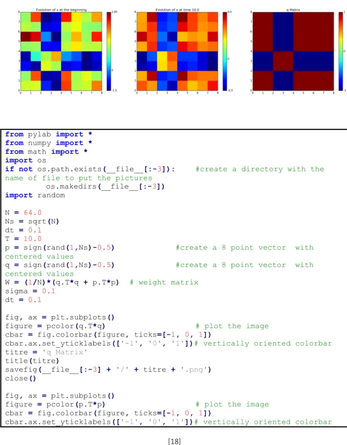
We see that the initial pattern (which is near to p.T*p) converge to p.T*p. (c) Evolution with two patterns stored in weight matrix
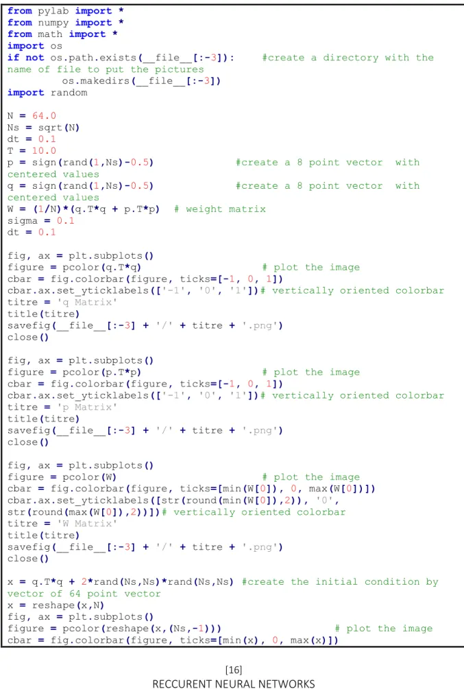
from pylab import * from numpy import * from math import * import os
if not os.path.exists(__file__[:-3]): #create a directory with the name of file to put the pictures
os.makedirs(__file__[:-3]) import random N = 64.0 Ns = sqrt(N) dt = 0.1 T = 10.0
p = sign(rand(1,Ns)-0.5) #create a 8 point vector with centered values
q = sign(rand(1,Ns)-0.5) #create a 8 point vector with centered values
W = (1/N)*(q.T*q + p.T*p) # weight matrix
sigma = 0.1
dt = 0.1
fig, ax = plt.subplots()
figure = pcolor(q.T*q) # plot the image
cbar = fig.colorbar(figure, ticks=[-1, 0, 1])
cbar.ax.set_yticklabels(['-1', '0', '1'])# vertically oriented colorbar
titre = 'q Matrix'
title(titre)
savefig(__file__[:-3] + '/' + titre + '.png')
close()
fig, ax = plt.subplots()
figure = pcolor(p.T*p) # plot the image
cbar = fig.colorbar(figure, ticks=[-1, 0, 1])
cbar.ax.set_yticklabels(['-1', '0', '1'])# vertically oriented colorbar
titre = 'p Matrix'
title(titre)
savefig(__file__[:-3] + '/' + titre + '.png')
close()
fig, ax = plt.subplots()
figure = pcolor(W) # plot the image
cbar = fig.colorbar(figure, ticks=[min(W[0]), 0, max(W[0])])
cbar.ax.set_yticklabels([str(round(min(W[0]),2)), '0',
str(round(max(W[0]),2))])# vertically oriented colorbar
titre = 'W Matrix'
title(titre)
savefig(__file__[:-3] + '/' + titre + '.png')
close()
x = q.T*q + 2*rand(Ns,Ns)*rand(Ns,Ns) #create the initial condition by vector of 64 point vector
x = reshape(x,N)
fig, ax = plt.subplots()
figure = pcolor(reshape(x,(Ns,-1))) # plot the image
cbar.ax.set_yticklabels([str(round(min(x),2)), '0',
str(round(max(x),2))])# vertically oriented colorbar
titre = 'Evolution of x at the beginning'
title(titre)
savefig(__file__[:-3] + '/' + titre + '.png')
close()
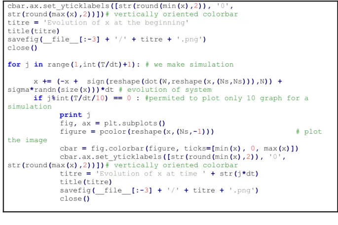
for j in range(1,int(T/dt)+1): # we make simulation
x += (-x + sign(reshape(dot(W,reshape(x,(Ns,Ns))),N)) +
sigma*randn(size(x)))*dt # evolution of system
if j%int(T/dt/10) == 0 : #permited to plot only 10 graph for a simulation
print j
fig, ax = plt.subplots()
figure = pcolor(reshape(x,(Ns,-1))) # plot the image
cbar = fig.colorbar(figure, ticks=[min(x), 0, max(x)])
cbar.ax.set_yticklabels([str(round(min(x),2)), '0',
str(round(max(x),2))])# vertically oriented colorbar
titre = 'Evolution of x at time ' + str(j*dt)
title(titre)
savefig(__file__[:-3] + '/' + titre + '.png')
close()
Matrix W seems to be the weight difference between patterns for each connections. If we start with a patterns near to the pattern that we want, system converge through it.
(d) General rule
In the article “Hertz, John A., Anders S. Krogh, and Richard G. Palmer. Introduction to the theory of neural computation”, researchers saw that for 1000 connections in the Hopfield network, we have 138 patterns can be storage. So here we have 64 connection: we can store 8 patterns! For the code, if I replace sign by tanh, my pattern converge with less precision and all the matrix converge to zero.
from pylab import * from numpy import * from math import * import os
if not os.path.exists(__file__[:-3]): #create a directory with the name of file to put the pictures
os.makedirs(__file__[:-3]) import random N = 64.0 Ns = sqrt(N) dt = 0.1 T = 10.0
p = sign(rand(1,Ns)-0.5) #create a 8 point vector with centered values
q = sign(rand(1,Ns)-0.5) #create a 8 point vector with centered values
W = (1/N)*(q.T*q + p.T*p) # weight matrix
sigma = 0.1
dt = 0.1
fig, ax = plt.subplots()
figure = pcolor(q.T*q) # plot the image
cbar = fig.colorbar(figure, ticks=[-1, 0, 1])
cbar.ax.set_yticklabels(['-1', '0', '1'])# vertically oriented colorbar
titre = 'q Matrix'
title(titre)
savefig(__file__[:-3] + '/' + titre + '.png')
close()
fig, ax = plt.subplots()
figure = pcolor(p.T*p) # plot the image
cbar = fig.colorbar(figure, ticks=[-1, 0, 1])
titre = 'p Matrix'
title(titre)
savefig(__file__[:-3] + '/' + titre + '.png')
close()
fig, ax = plt.subplots()
figure = pcolor(W) # plot the image
cbar = fig.colorbar(figure, ticks=[min(W[0]), 0, max(W[0])])
cbar.ax.set_yticklabels([str(round(min(W[0]),2)), '0',
str(round(max(W[0]),2))])# vertically oriented colorbar
titre = 'W Matrix'
title(titre)
savefig(__file__[:-3] + '/' + titre + '.png')
close()
x = q.T*q + 2*rand(Ns,Ns)*rand(Ns,Ns) #create the initial condition by vector of 64 point vector
x = reshape(x,N)
fig, ax = plt.subplots()
figure = pcolor(reshape(x,(Ns,-1))) # plot the image
cbar = fig.colorbar(figure, ticks=[min(x), 0, max(x)])
cbar.ax.set_yticklabels([str(round(min(x),2)), '0',
str(round(max(x),2))])# vertically oriented colorbar
titre = 'Evolution of x at the beginning'
title(titre)
savefig(__file__[:-3] + '/' + titre + '.png')
close()
for j in range(1,int(T/dt)+1): # we make simulation
I = reshape(dot(W,reshape(x,(Ns,Ns))),N) for i in I : i = tanh(i)
x += (-x + I)*dt # evolution of system
if j%int(T/dt/10) == 0 : #permited to plot only 10 graph for a simulation
print j
fig, ax = plt.subplots()
figure = pcolor(reshape(x,(Ns,-1))) # plot the image
cbar = fig.colorbar(figure, ticks=[min(x), 0, max(x)])
cbar.ax.set_yticklabels([str(round(min(x),2)), '0',
str(round(max(x),2))])# vertically oriented colorbar
titre = 'Evolution of x at time ' + str(j*dt)
title(titre)
savefig(__file__[:-3] + '/' + titre + '.png')