Department of Economics
Working Paper No. 221
Adaptive Shrinkage in Bayesian Vector
Autoregressive Models
Martin Feldkircher
Florian Huber
Adaptive shrinkage in Bayesian vector
autoregressive models
Florian Huber1 and Martin Feldkircher∗2
1Vienna University of Economics and Business 2Oesterreichische Nationalbank (OeNB)
Abstract
Vector autoregressive (VAR) models are frequently used for forecasting and pulse response analysis. For both applications, shrinkage priors can help im-proving inference. In this paper we derive the shrinkage prior of Griffin et al.
(2010) for the VAR case and its relevant conditional posterior distributions. This framework imposes a set of normally distributed priors on the autoregressive co-efficients and the covariances of the VAR along with Gamma priors on a set of local and global prior scaling parameters. This prior setup is then generalized by introducing another layer of shrinkage with scaling parameters that push cer-tain regions of the parameter space to zero. A simulation exercise shows that the proposed framework yields more precise estimates of the model parameters and impulse response functions. In addition, a forecasting exercise applied to US data shows that the proposed prior outperforms other specifications in terms of point and density predictions.
Keywords: Normal-Gamma prior, density predictions, hierarchical modeling
JEL Codes: C11, C30, C53, E52.
∗
Corresponding author: Florian Huber, Vienna University of Economics and Business. E-mail:
[email protected]. We would like to thank Gregor Kastner and Philipp Piribauer for helpful comments and
suggestions. Any views expressed in this paper represent those of the authors only and not necessarily of the Oesterreichische Nationalbank or the Eurosystem.
1 Introduction
Macroeconomists often face situations where the number of available observations is low relative to the number of potentially available time series. Especially in vector au-toregressive models (VARs), the number of parameters quickly becomes prohibitively large even if the number of time series included is moderate. This translates into severe overfitting issues that ultimately lead to imprecise out-of-sample predictions.
In this study, we consider VAR models that describe the law of motion of a m
-dimensional vectoryt fort= 1, . . . , T,
yt=A1yt−1+· · ·+Apyt−p+εt, (1.1)
withAj (j = 1, . . . , p) being a set of m×m coefficient matrices associated with the
plags of yt. The errors in εt are normally distributed with zero mean and
variance-covariance matrix Σ, which is a symmetric and positive definite matrix. The total
number of autoregressive parameters isk = m(mp), and thus rises rapidly with the
number of endogenous variablesm and the number of lagged endogenous variables
included. In addition, thev = m(m2−1) covariances and the m variances also have to
be inferred from a possibly limited amount of data.
Taking a Bayesian stance, several ways of estimating the model inEq. (1.1) have
been proposed. Most prominently, Litterman (1979, 1986) and Doan et al. (1984)
advocate a set of prior distributions that center the whole system on a multivariate random walk process. This implies that coefficient matrices of lag orders greater than unity are pushed towards a zero matrix. By specifiying appropriate prior variance-covariance matrices, these priors induce sparsity by imposing more shrinkage to co-efficients associated with higher lag orders, capturing the notion that the most recent
past seems to be more important to predictyt. Other variations, like the sum of
co-efficients (Doan et al., 1984) or the dummy initial observation prior (Sims, 1993),
provide several options to alleviate the curse of dimensionality in a VAR. Especially in large models, variants of the priors discussed have been particularly successful in forecasting applications (Ba´nbura et al.,2010;Carriero et al.,2009;2012;Giannone et al.,2014).
More recently, the dependence and sensitivity of the aforementioned priors with respect to a lower dimensional vector of hyperparameters led to the development of hierarchical models that introduce another layer of priors on the hyperparameters.
For instance,George et al.(2008) propose stochastic search variable selection (SSVS)
priors (seeGeorge and McCulloch,1993) that impose a mixture normal prior on each
regression coefficient in the VAR. In another contribution,Giannone et al.(2015)
ex-tend the work ofSims and Zha(1998) and propose a hierarchical prior that estimates
the hyperparameters of the Minnesota, the sum of coefficients and the dummy initial observation prior in a data-based fashion. They show that this hierarchical setup
per-forms well as compared to non-hierarchical priors and models estimated by means of maximum likelihood.
The SSVS prior and the prior of Giannone et al.(2015) both deal with the
prob-lem of hyperparameter selection in an elegant way, integrating out the hyperparam-eters in a Bayesian fashion. However, both specifications share a trade-off in terms of flexibility and complexity. For instance, the Minnesota prior induces a Kronecker structure on the likelihood, leading to symmetric shrinkage across equations. This implies that each equation is deemed to feature the same set of predictors. On the other hand, while the SSVS prior allows for different explanatory variables across equations, this prior only discriminates between inclusion and exclusion, ruling out cases in between. Moreover, the SSVS prior, although possessing convenient
theoret-ical properties (Bhattacharya et al., 2015), imposes a severe computational burden
if the model space to explore is large. This is typically the case in VAR applications where the number of parameters grows exponentially with the numbers of variables
included.1
Another strand of the literature proposes double exponential prior on the
coeffi-cients, leading to the Bayesian variant of the LASSO (Park and Casella,2008). Gefang
(2014) propose a Bayesian LASSO for VAR models, showing that forecast results tend
to be similar to the ones obtained from standard Minnesota-type priors. However, it is worth noting that a major limitation of the double exponential prior is its lack of flexibility. This prior ultimately relies on a single hyperparameter, implying that the specific choice of this parameter has serious implications for inference. To provide
more flexibility, Griffin et al. (2010) introduce a Normal-Gamma prior that solves
several shortcomings of the priors discussed hitherto. This prior, being a general-ization of the double exponential prior, possesses far richer shrinkage properties as compared to alternative solutions.
The main contribution of this paper is to generalize the Normal-Gamma prior of Griffin et al. (2010) to the VAR case. We impose a conditionally Gaussian prior on each autoregressive coefficient in the VAR with idiosyncratic and global scaling factors. For these, we impose a set of Gamma priors. Moreover and since prior infor-mation on the sparsity of the error variances is typically not available, we also impose a set of Normal-Gamma priors on the covariances. Under this prior setup, we devise conditional posterior distributions for all parameters, leading to a relatively simple Metropolis-within-Gibbs sampling scheme. Our prior setup provides two sources of flexibility. First, the full coefficient matrix of the VAR is pushed towards a zero matrix
a priori, thus providingglobal shrinkage. Second, a Gamma prior on the coefficients
induces a fat-tailed marginal prior ensuring that non-zero signals are not too strongly
put to zero (Polson and Scott,2010). To provide additional flexibility, we also extend
the standard Normal-Gamma prior by introducing additional global shrinkage param-eters that exhibit symmetric shrinkage on certain regions of the parameter space.
We illustrate the merits of our approach by performing a set of simulation studies. Comparing the performance of our model with a set of competing models reveals that our approach improves upon competing models in terms of root mean square forecast errors and predictive likelihoods. To assess how our model performs in a typical real-data application we forecast output growth, wage growth, inflation and short-term interest rates in the US. Our modeling approach delivers excellent point and density predictions, emphasizing the accuracy gains stemming from the increased flexibility of the prior distribution adopted. In terms of density forecasts, these can even fur-ther improved by introducing ”column-wise” shrinkage to the Normal-Gamma spec-ification. The merits of the Normal-Gamma framework also carry over to structural analysis. Looking at a contractionary US monetary policy shock, the NG-VAR yields responses that are consistent with established findings in the literature.
The paper is organized as follows. Section 2 introduces some useful notation, de-scribes the model and our prior setup employed. In addition, the relevant conditional posterior distributions and the MCMC algorithm are outlined. Section 3 presents the main results of the simulation study. Section 4 presents a forecasting application for the US economy, and Section 5 extends the Normal-Gamma prior. Finally, the last section concludes the paper.
2 Econometric framework
This section proposes the Normal-Gamma prior for VAR models. The first subsection introduces additional notation that vastly simplifies prior implementation. After pro-viding some information on the specific prior setup adopted for the autoregressive coefficients of the model, we proceed by specifying a prior on the covariances leading to a sparse representation of the variance-covariance matrix of the model.
2.1 The model
We set the stage by rewriting the model in Eq. (1.1) as a multivariate regression
model withxt= (yt−1, . . . ,y t−p) and A= (A1, . . . ,Ap), yt=Axt+εt. (2.1)
Rewriting in terms of full-data matrices yields
Y =XA+ε, (2.2)
withY = (y1, . . . ,yT)
, X = (x1, . . . ,xT) and ε = (ε1, . . . ,εt). The matricesY and
Several possible factorizations of the variance-covariance matrix are available
(see, among others, Pourahmadi, 1999; Smith and Kohn, 2002). In this paper we
followGeorge et al.(2008) and factorizeΣas
Σ−1 =HH. (2.3)
Here, H denotes an upper triangular matrix. We denote a typical non-zero
off-diagonal element ashij and a typical main diagonal element is denoted asτii. Often,
economists are interested in identifying structural shocks and a prominent way of
achieving identification is by using a Cholesky decomposition forΣ. Such a
decom-position implies zero impact restrictions of the shocks and is sensitive to the ordering
of the variables inyt, which has to be justified based on economic grounds. As an
al-ternative to pre-selected restrictions,George et al. (2008) propose using restrictions
that are supported by the data itself, which we accomplish by placing the Normal-Gamma prior also on the variance-covariance matrix.
2.2 Prior setup
Traditionally, normally distributed priors are imposed on A and inverted Wishart
priors are used for Σ. However, inverted Wishart priors make it difficult to elicit
sophisticated prior structures on the covariances. Thus, we impose inverted Gamma
priors on the squared main diagonal elements ofHand normally distributed priors on
allhij. All Gaussian priors used in this paper depend on idiosyncratic scaling factors
that effectively control the degree of shrinkage for each coefficient. In addition, a
global hyperparameter shrinks the full coefficient matrix towards zero.
Let us denote the stackedmk-dimensional vector of autoregressive coefficients as
α=vec(A)with typical elementαi. The marginal prior distribution for each element
ofαis given by the following scale mixture of normals prior (Griffin et al.,2010),
p(αi) =
N(0, ψi)dG(ψi). (2.4)
G(ψi)is a mixing distribution, which in our case is specified as a Gamma distribution.
We can state this prior in its hierarchical form as
αi|ψi ∼ N(0,2/λ2ψψi), ψi ∼ G(ϑψ, ϑψ), (2.5)
with ϑψ and λψ being hyperparameters chosen by the researcher. Equation (2.5)
implies that the prior on each regression coefficient is centered on zero conditional on
an idiosyncratic scaling parameterψi. This entails an individual degree of shrinkage
for each αi, irrespective of the size of the regression coefficient. Moreover, λ2ψ is
a global shrinkage parameter that shrinks the full coefficient vector towards zero (Polson and Scott,2010).
Griffin et al.(2010) show that the unconditional prior density can be obtained by
integrating outψi ofEq. (2.5). It can be shown that the variance of the corresponding
density is negatively related to λ2φ and the excess kurtosis depends on ϑψ. More
specifically, ifϑψ decreases, the prior places more mass on zero but at the same time,
the tails of the density become heavier. This yields the convenient property that if the likelihood strongly suggests non-zero values of a given parameter, a very tight prior (i.e.,ϑψ set to a low value and λ2ψ set to a high value) still provides enough flexibility to let the data speak. By contrast, a standard Minnesota prior would exert too much shrinkage, effectively pushing the posterior towards the prior.
For the free off-diagonal elements ofH we also impose a Normal-Gamma prior,
hij|φij ∼ N(0,2/λ2φφij), φij ∼ G(ϑφ, ϑφ). (2.6)
As before,ϑφandλ2φare scalar hyperparameters controlling the tightness of the prior.
The same intuition as inEq. (2.5)applies. The global shrinkage parameterλ2
φpushes
all covariances inH towards zero. The shrinkage parameterφij provides the
flexibil-ity needed to allow for non-zero covariances even if the global shrinkage parameter exerts a strong degree of overall shrinkage. Thus, if the data generating process
as-sumes thatH is sparse, our prior setup is capable of detecting covariances that are
truly zero while covariances unequal to zero are not too strongly pushed towards
zero. By contrast, a standard Minnesota prior typically assumes that Σis a diagonal
matrix a priori and thus shrinks all covariances towards zero.
We proceed by imposing additional priors on the hyperparameters of the prior
de-scribed byEq. (2.5)andEq. (2.6). Since our prior setup leads to the Bayesian LASSO
(Park and Casella,2008) ifϑψ =ϑφ= 1, we impose an exponentially distributed prior onϑk, k ∈ {ψ, φ}centered on unity,
ϑk ∼Exp(1). (2.7)
Moreover, we impose a Gamma prior onλk with hyperparametersck0 and ck1,
λk∼ G(ck0, ck1). (2.8)
We setck0 =ck1 = 0.01for all kto render this prior effectively non-influential for λk.
The final ingredient missing is the prior on the main diagonal elements of H,
denoted asτ2
ii, where we again impose a gamma distributed prior
τii2 ∼ G(ai, bi), i= 1, . . . , m. (2.9)
Similar to the hyperparameter setup forλk, ai andbi are set equal to 0.01for alli to
obtain a non-informative prior distribution forτ2
2.3 Posterior distributions
Combining the prior distributions with the likelihood yields the posterior distribution. In our case, the conditional posterior distributions for most parameters are available in closed form, suggesting a relatively straightforward Markov chain Monte Carlo (MCMC) algorithm that iteratively simulates from the conditional posterior distribu-tions.
The conditional posterior distribution of the autoregressive coefficientsαis given
by
α|H,ψ,φ, λψ,Y ∼ N(α,Vα), (2.10)
where ψ = (ψ1, . . . , ψmk) and conditional on H, the corresponding
hyperparame-ters carry no additional information. The posterior mean α and variance Vα take
standard forms (Kadiyala et al.,1997;Karlsson,2013),
Vα =
(HH)⊗(XX) +V−α1 −1
(2.11)
withVα being amk×mk dimensional diagonal matrix with
[Vα]ii= 2/λ2ψψi. (2.12)
Here the notation[•]iiselects thei, ith element of a given matrix. The posterior mean
αis given by
α=Vα[(HH)⊗(XX) ˆα]. (2.13)
ˆ
αdenotes the least squares estimate ofα.
It can be shown2that the conditional posterior ofψ
i follows a generalized inverse
Gaussian (GIG) distribution,
ψi|ϑψ, λ2ψ, αi ∼ GIG(ϑψ− 1 2, ϑψλ 2 ψ, α 2 i). (2.14)
The density of the GIG distribution is given by
f(x)∝xn−1e−(ax+b/x)/2. (2.15)
The parameters of the GIG distribution area, b > 0and n∈R.
Unfortunately, the conditional posterior ofϑψ has no well known form. This
ren-ders a Gibbs sampling step impossible. Fortunately, a Metropolis Hastings step can be implemented in a straightforward fashion, where the acceptance probability equals
min 1,p(ϑ ∗ ψ) p(ϑψ) (ϑ∗ ψλ 2 ψ/2) mkϑ∗ ψ (ϑψλ2ψ/2)mkϑψ Γ(ϑ∗ ψ) Γ(ϑψ) mk j=1 ψj ϑ∗ ψ−ϑψ , (2.16)
with Γ(•) denoting the Gamma function and ϑ∗
ψ being the proposed value of ϑψ.
Equation (2.16) implies that the acceptance probability equals the ratio of the prior
density onψi times the prior onϑψ, denoted byp(ϑψ).
The conditional posterior ofλ2
ψ is of a well-known form, namely a Gamma
distri-bution, λ2ψ|ϑψ,ψ ∼ G cψ0+ϑψk, cψ0+ϑψ/2 mk j=1 ψj . (2.17)
The free off-diagonal blocks of H, denoted as hj = (h1j, . . . , hj−1j), for j =
2, . . . , m, follow a Gaussian distribution given by (George et al.,2008),
hj|φ, λφ,A,Y ∼ N(hj,Vjh), (2.18)
withφ= (φ12, φ13, φ23, . . . , φm−1m) and posterior variance being equal to
Vjh=
Ωj−1+V−jh1
−1
. (2.19)
Here, we letΩj−1 denote the upper left(j −1)×(j−1)submatrix ofΩ(A) = (Y −
XA)(Y −XA), with typical elementωij, andVjh is a prior variance matrix with
typical element given by
[Vjh]ii= 2/λ2φφij. (2.20)
The posterior mean is
hj =−τjjVjhωj, (2.21)
whereωj = (ω1j, . . . , ωj−1j).
As shown in George et al. (2008), the conditional posterior distribution of τ2
jj is Gamma distributed,
τjj2|φ, λφ,A,Y ∼ G(ai+T /2, κi). (2.22)
The rate parameterκi is given by
κi =
a1+ωij/2 for i= 1
ai+ (ωii−ωi(Ωi−1+V−ih1)
−1ωi fori= 2, . . . , m. (2.23)
Similar to the elements of the prior related toA, the conditional posterior distribution
ofφij is GIG distributed with
φij|ϑφ, λφ, hij ∼ GIG(ϑφ−
1
2, ϑφλφ, h
2
ij) (2.24)
As in the case of the conditional posterior of ϑψ, the conditional posterior of ϑφ
Hastings step to simulate from the target distribution. Again, the probability of
ac-cepting a candidate drawϑ∗φ depends on the ratio of the prior densities onφij times
the prior. More specifically, the probability to acceptϑφequals
min 1,π(ϑ ∗ φ) π(ϑφ) (ϑ∗φλ2φ/2)vϑ∗φ (ϑφλ2φ/2) vϑφ Γ(ϑ∗φ) Γ(ϑφ) m−1 i=1 m j=2 φij ϑ∗ φ−ϑφ . (2.25)
The final quantity needed is the global shrinkage parameter associated with the
elements in H. Similar to Eq. (2.17), it is possible to show that the conditional
posterior is Gamma distributed,
λφ|ϑφ,φ∼ G cφ0+ϑφv, cφ0+ϑφ/2 m−1 i=1 m j=2 φij . (2.26)
A relatively straightforward MCMC scheme can be devised by iteratively drawing
from the conditional posterior distributions described in Eq. (2.10) to Eq. (2.26).
More specifically, the MCMC algorithm consists of the following steps
Step 0 Initialize all parameters of the model by using the corresponding OLS es-timates or by drawing from the prior
Step 1 DrawαusingEq. (2.10)
Step 2 Drawhj for j = 2, . . . , mfromEq. (2.18)
Step 3 Drawτjj forj = 1, . . . , mfrom Eq. (2.22)and computeΣ
−1
=HH
Step 4 Draw ψi for i = 1, . . . , k element-wise from Eq. (2.14) and φij for i =
1, . . . , m−1; j = 2, . . . , mfromEq. (2.24)
Step 5 Drawλ2ψ and λ2φfrom Eq. (2.17)and Eq. (2.26).
Step 6 Drawϑψ andϑφ with a univariate random walk Metropolis Hastings step
For Step 6, following Griffin et al. (2010), the proposal adopted is λ
j = exp(ςjz)λj
for j ∈ {ψ, φ}. ςj is a tuning parameter set such that the acceptance probability lies
between 20 and 40 percent and z is a standard normal random variable. For the
simulation study and the empirical application that follows we repeat the algorithm 30,000 times and discard the first 15,000 as burn-in. Typical convergence diagnostics suggest that the Markov chain rapidly converges towards the target distribution.
3 Simulation results
In this section, we evaluate the performance of our model by means of a simple
simulation exercise. We followGeorge et al.(2008) and simulate a moderately sized
VAR(1) model withT = 150andT = 250and six endogenous variables. Furthermore,
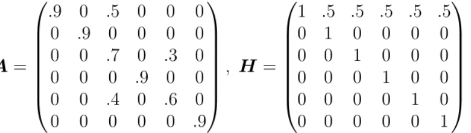
we assume that the true coefficient matricesAand H are sparse. More specifically,
the true values ofAand H are
A= .9 0 .5 0 0 0 0 .9 0 0 0 0 0 0 .7 0 .3 0 0 0 0 .9 0 0 0 0 .4 0 .6 0 0 0 0 0 0 .9 , H = 1 .5 .5 .5 .5 .5 0 1 0 0 0 0 0 0 1 0 0 0 0 0 0 1 0 0 0 0 0 0 1 0 0 0 0 0 0 1 . (3.1)
In our simulation exercise we investigate the differences between the posterior
me-dian and the true value of A and the free off-diagonal elements of H by means of
root mean square errors (RMSE). As competing models, we include a simple BVAR coupled with a Minnesota prior where the hyperparameter of the Minnesota prior is chosen by maximizing the marginal likelihood over a grid of possible hyperparam-eters and a model estimated under a flat prior (i.e., estimated by maximum
likeli-hood). Since Griffin et al. (2010) emphasized the importance of the shrinkage
pa-rametersϑψ and ϑφ, we first evaluate the performance of our model with respect to
ϑψ ∈ {0.01,0.05,0.1,0.3,0.6,0.8,0.9,1,2,3}, while keepingϑφ= 0.1fixed.3 In the next
step, we choose the value ofϑψ that yields the minimum RMSE and investigate the
impact ofϑφ (evaluated over the same grid of possible values). All VARs used in the
simulation feature a single lag of the endogenous variables and no constant.
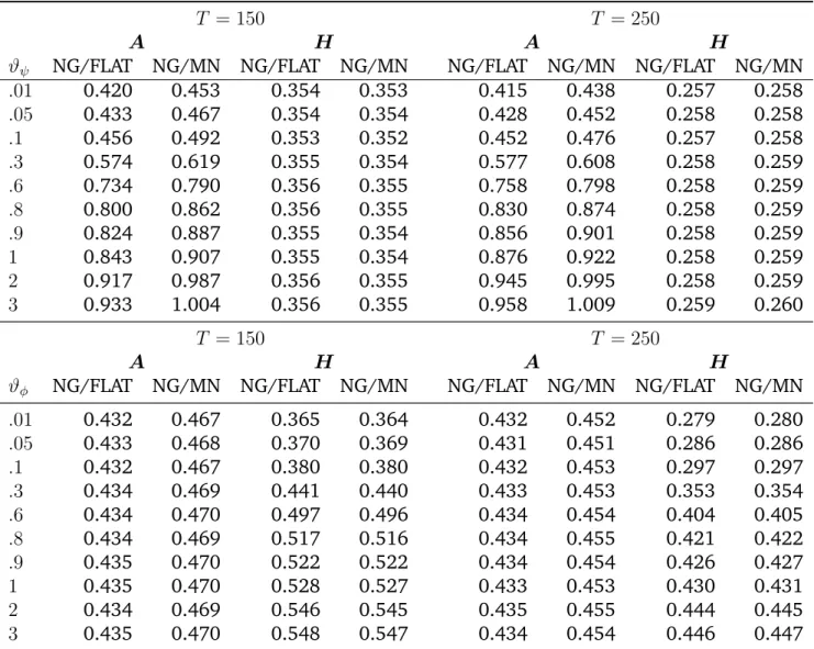
Table1depicts the findings of our simulation exercise. The first four columns
re-fer to the results obtained by simulatingT = 150observations from the VAR model
and the final four columns refer to a situation withT = 250 observations. The
fig-ures in the first two columns present the relative RMSEs of the Normal-Gamma VAR (NG) against a VAR estimated with a flat prior (FLAT) and relative to a VAR with a
Minnesota prior (MN) forA, while the numbers in column three and four depict the
results for the free off-diagonal elements inH. Numbers smaller than unity indicate
outperformance of the NG-VAR relative to the other models.
3This value is based on integrating outϑ
T = 150 T = 250
A H A H
ϑψ NG/FLAT NG/MN NG/FLAT NG/MN NG/FLAT NG/MN NG/FLAT NG/MN
.01 0.420 0.453 0.354 0.353 0.415 0.438 0.257 0.258 .05 0.433 0.467 0.354 0.354 0.428 0.452 0.258 0.258 .1 0.456 0.492 0.353 0.352 0.452 0.476 0.257 0.258 .3 0.574 0.619 0.355 0.354 0.577 0.608 0.258 0.259 .6 0.734 0.790 0.356 0.355 0.758 0.798 0.258 0.259 .8 0.800 0.862 0.356 0.355 0.830 0.874 0.258 0.259 .9 0.824 0.887 0.355 0.354 0.856 0.901 0.258 0.259 1 0.843 0.907 0.355 0.354 0.876 0.922 0.258 0.259 2 0.917 0.987 0.356 0.355 0.945 0.995 0.258 0.259 3 0.933 1.004 0.356 0.355 0.958 1.009 0.259 0.260 T = 150 T = 250 A H A H
ϑφ NG/FLAT NG/MN NG/FLAT NG/MN NG/FLAT NG/MN NG/FLAT NG/MN
.01 0.432 0.467 0.365 0.364 0.432 0.452 0.279 0.280 .05 0.433 0.468 0.370 0.369 0.431 0.451 0.286 0.286 .1 0.432 0.467 0.380 0.380 0.432 0.453 0.297 0.297 .3 0.434 0.469 0.441 0.440 0.433 0.453 0.353 0.354 .6 0.434 0.470 0.497 0.496 0.434 0.454 0.404 0.405 .8 0.434 0.469 0.517 0.516 0.434 0.455 0.421 0.422 .9 0.435 0.470 0.522 0.522 0.434 0.454 0.426 0.427 1 0.435 0.470 0.528 0.527 0.433 0.453 0.430 0.431 2 0.434 0.469 0.546 0.545 0.435 0.455 0.444 0.445 3 0.435 0.470 0.548 0.547 0.434 0.454 0.446 0.447
Notes:The figures refer to the relative RMSE of the vector autoregressive model coupled with a Normal-Gamma prior (NG) against either a VAR estimated with maximum likelihood, i.e., a flat prior (FLAT), or with a Minnesota prior (MN). The first part of the Table corresponds toT = 150 and the second part toT = 250. Results are shown for the autoregressive coefficientsAand the free off-diagonal elements inH. Results based on 10,000 posterior draws out of a chain of 20,000 draws and 150 replications of the simulation exercise.
The upper part of Table1suggests that the specific value ofϑψ proves to be quite
influential in terms of improving the precision of parameter estimates forA. Smaller
values are typically associated with lower RMSEs, indicating that the shrinkage in-duced through the prior is not becoming excessively large, even for relatively low
values ofϑψ. Note that both the BVAR with the Minnesota prior and the flat prior VAR
are outperformed by large margins. While the parameter estimates of the flat prior VAR model are characterized by a large amount of non-zero values, even if the true parameters equal zero, the Minnesota prior tends to excessively shrink the parameter matrix, effectively pushing estimates for parameters that are non-zero towards zero. This leads to inferior performance and larger RMSEs.
The results for Adirectly carry over to the estimates of the free off-diagonal
ele-ments ofH. Here it can be seen that the NG prior strongly improves the accuracy of
the estimates, outperforming the estimate obtained from a flat prior VAR by roughly 60%. The accuracy gains are comparable when the model is benchmarked against the Minnesota prior, suggesting that in terms of estimating the covariance matrix, the Minnesota prior and the VAR coupled with a flat prior both perform relatively poor as compared to the NG-VAR.
Comparing the results betweenT = 150and T = 250suggests that there are no
discernible differences in terms of the performance of the NG-VAR. This rather sur-prising finding could be due to the fact that our simulation design mirrors a situation where the number of parameters is moderate relative to the length of the data set. We conjecture that our model improves even more if the number of parameters is
increased relative to the length of the dataset.4
Finally, the upper part of Table1 suggests that varying ϑψ tends to be important
for the estimates of A, the impact on the estimates of H is negligible. This finding
also holds true in the case where we varyϑφ.
To gain further insights on where the accuracy gains stem from,Fig. 1depicts the
posterior distributions of thehijs along with the actual value (in black), the posterior
median (in orange) and the ML estimate (in blue). In addition, we impose the prior
described in the previous section onϑφandϑψ.
4For instance, if we increase the number of lagged endogenous variables the outperformance of the NG-VAR is even more pronounced. The specific results are available upon request.
0.5
0.5 0
0.5 0 0
0.5 0 0 0
0.5 0 0 0 0
Notes: Posterior distribution of the free elements of H. The red line corresponds to the actual value, the orange line to the posterior median and the blue line to the estimate obtained by using a flat prior. The numbers below the figure are the actual values.
Fig. 1: Posterior distribution of H
As can be seen from the figure, the NG-VAR successfully shrinks the covariances towards zero. The standard VAR model produces estimates that are often non-zero, even if the true parameter equals zero. Note that in the case of non-zero covariances, the NG-VAR does not push too strongly towards zero, providing enough flexibility in the presence of strong global shrinkage.
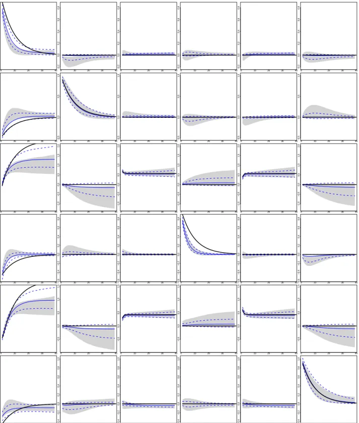
The impulse response functions (IRF) for the NG-VAR along with the impulses
obtained from a flat prior VAR are shown inFig. 2. The dashed blue lines represent
of the NG-VAR impulse response functions. For comparison, the gray shaded areas correspond to the 16th and 84th credible sets obtained from a flat prior VAR. The solid black line denotes the true value of the simulated response.
An interesting case arises if the simulated response of a given variable is zero. Here, inference under the flat prior can be quite misleading. For example in the
first row, first column ofFig. 1the flat prior indicates responses that are significantly
different from zero (i.e., zero is not included in the gray shaded area). The same applies to the response shown in the sixth row, second column. By contrast, the NG-VAR, although not perfectly, shrinks these responses towards zero.
More generally, credible sets for impulse responses based on the NG-VAR are much tighter compared to the ones related to the flat prior VAR. For example, responses in the first column show much tighter credible sets and responses under the flat prior are sometimes way off the simulated responses. In very few cases, the simulated response lies outside the credible set of the NG-VAR (e.g., row 4 and column 4). Even for these cases the NG-VAR improves upon the flat prior VAR and the associated median response is closer to the simulated response compared to the one generated by the flat prior VAR.
0 10 20 30 40 −0.2 0.0 0.2 0.4 0.6 0.8 0 10 20 30 40 −0.2 0.0 0.2 0.4 0.6 0.8 0 10 20 30 40 −0.2 0.0 0.2 0.4 0.6 0.8 0 10 20 30 40 −0.2 0.0 0.2 0.4 0.6 0.8 0 10 20 30 40 −0.2 0.0 0.2 0.4 0.6 0.8 0 10 20 30 40 −0.2 0.0 0.2 0.4 0.6 0.8 0 10 20 30 40 −0.5 0.0 0.5 1.0 0 10 20 30 40 −0.5 0.0 0.5 1.0 0 10 20 30 40 −0.5 0.0 0.5 1.0 0 10 20 30 40 −0.5 0.0 0.5 1.0 0 10 20 30 40 −0.5 0.0 0.5 1.0 0 10 20 30 40 −0.5 0.0 0.5 1.0 0 10 20 30 40 −1.0 −0.5 0.0 0.5 1.0 1.5 2.0 0 10 20 30 40 −1.0 −0.5 0.0 0.5 1.0 1.5 2.0 0 10 20 30 40 −1.0 −0.5 0.0 0.5 1.0 1.5 2.0 0 10 20 30 40 −1.0 −0.5 0.0 0.5 1.0 1.5 2.0 0 10 20 30 40 −1.0 −0.5 0.0 0.5 1.0 1.5 2.0 0 10 20 30 40 −1.0 −0.5 0.0 0.5 1.0 1.5 2.0 0 10 20 30 40 −0.6 −0.4 −0.2 0.0 0.2 0.4 0.6 0.8 0 10 20 30 40 −0.6 −0.4 −0.2 0.0 0.2 0.4 0.6 0.8 0 10 20 30 40 −0.6 −0.4 −0.2 0.0 0.2 0.4 0.6 0.8 0 10 20 30 40 −0.6 −0.4 −0.2 0.0 0.2 0.4 0.6 0.8 0 10 20 30 40 −0.6 −0.4 −0.2 0.0 0.2 0.4 0.6 0.8 0 10 20 30 40 −0.6 −0.4 −0.2 0.0 0.2 0.4 0.6 0.8 0 10 20 30 40 −0.5 0.0 0.5 1.0 1.5 0 10 20 30 40 −0.5 0.0 0.5 1.0 1.5 0 10 20 30 40 −0.5 0.0 0.5 1.0 1.5 0 10 20 30 40 −0.5 0.0 0.5 1.0 1.5 0 10 20 30 40 −0.5 0.0 0.5 1.0 1.5 0 10 20 30 40 −0.5 0.0 0.5 1.0 1.5 0 10 20 30 40 −0.4 −0.2 0.0 0.2 0.4 0.6 0.8 1.0 0 10 20 30 40 −0.4 −0.2 0.0 0.2 0.4 0.6 0.8 1.0 0 10 20 30 40 −0.4 −0.2 0.0 0.2 0.4 0.6 0.8 1.0 0 10 20 30 40 −0.4 −0.2 0.0 0.2 0.4 0.6 0.8 1.0 0 10 20 30 40 −0.4 −0.2 0.0 0.2 0.4 0.6 0.8 1.0 0 10 20 30 40 −0.4 −0.2 0.0 0.2 0.4 0.6 0.8 1.0
Notes: Posterior distribution of impulse responses of the VAR with NG prior (16th and 84th credible sets in dashed blue, median in solid blue) and a flat prior VAR (the shaded area represents the 16th and 84th credible interval). The solid black line corresponds to the true value of the simulated impulse responses. The rows represent the responses of variables one to six to the six orthogonalized shocks (in the columns). The numbers below the figure are the actual values. Results based on 5,000 posterior draws out of a chain of 15,000 posterior draws.
4 Application: Modeling US macroeconomy
This section applies the NG-VAR to a US macroeconomic dataset. The following sub-section provides a brief overview of the data used and the corresponding transforma-tions. In addition, information on the specification of the model and the competitors are provided. The second subsection presents the results of the forecasting exercise. 4.1 Data overview and model specification
We extend the data used in Smets and Wouters (2003) and Geweke and Amisano
(2012) to span the period from 1947Q2 to 2014Q4. Data are on quarterly basis and
comprise the log differences of investment, real GDP, wages, consumer prices and the Federal Funds Rate (FFR). The time period covered includes spikes associated with recessions, in particular so in the aftermath of World War II, around 1980 when US Fed chairman Paul Volcker started fighting inflation by aggressively, and in the af-termath of the global financial crisis. In light of the quarterly frequency of our data
we include p = 4 lags of the endogenous variables for all models considered. As
competitors, we include a Bayesian VAR with a Minnesota prior where the hyperpa-rameters are selected by maximizing the marginal likelihood over a grid of possible
values (Carriero et al., 2015). For the Minnesota prior we set the prior mean equal
to zero for all coefficients, because our data are assumed to be stationary. Since the
Bayesian LASSO is nested within our approach if we restrict ϑψ = ϑφ = 1, we also
include it as a possible competing model (labeled LASSO). Finally, we include a flat prior VAR and a random walk without drift to asses how much the VAR structure improves predictions relative to a no-change forecast.
4.2 Forecasting results
In this section we provide results of the forecasting exercise. We evaluate both point forecasts and density forecasts by means of the RMSE and log predictive scores
(LPS)5, respectively. Forecasts are evaluated over a long hold-out sample spanning
the period from 1981Q1 to 2014Q1 and for the one-step and four-steps-ahead fore-cast horizon. We use a recursive forefore-casting design that consequently expands the initial estimation window until the end of the sample is reached.
5For a general discussion on the properties of the log predictive score, seeGeweke and Amisano (2010).
Sum of log predictive scores (LPS) relative to the random walk
One-step ahead Four-steps ahead
GDP Inflation Wages Fed Funds Overall GDP Inflation Wages Fed Funds Overall Normal-Gamma 17.53 8.70 2.00 14.05 35.44 5.30 1.73 2.02 10.97 15.60
LASSO 17.46 7.23 -3.09 8.79 23.66 6.60 1.82 -1.81 5.66 7.47 Minnesota 15.14 2.80 -7.80 9.31 13.92 5.58 -2.59 -3.75 6.50 2.69 Flat 13.38 2.48 -11.79 9.76 8.58 5.90 -4.51 -7.32 5.20 -1.15
Average root mean square forecast errors (RMSE) relative to the random walk One-step ahead Four-steps ahead GDP Inflation Wages Fed Funds GDP Inflation Wages Fed Funds Normal-Gamma 0.93 1.11 1.00 0.99 0.93 1.06 0.98 0.88
LASSO 0.95 1.24 1.01 1.03 0.96 1.17 1.00 0.90
Minnesota 0.96 1.30 1.04 1.02 0.96 1.19 1.01 0.91
Flat 1.03 1.40 1.06 1.02 0.99 1.35 1.03 0.95
Notes:NG stands for a vector autoregressive model coupled with a Normal-Gamma prior, LASSO for a VAR model with a double exponential prior, Minnesota for a VAR with a standard Minnesota prior and Flat refers to a flat prior VAR. GDP refers to real GDP per capita, Wages to real per capita wages, inflation to GDP inflation and Fed Funds to the federal funds rate. The bold figures indicate the best performing model for a given variable and time horizon.
Table 2: Out-of-sample performance relative to the random walk model in terms of the sum of log predictive scores (LPS) and the root mean square error (RMSE): 1981:Q1 to 2014:Q4
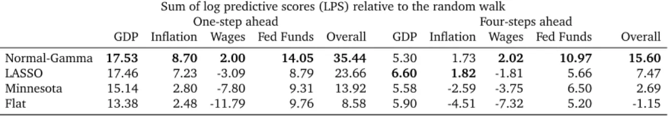
Table2summarizes the results. The top panel shows the differences of the sum of
log predictive scores over the hold-out sample with respect to the cumulative LPS of a simple random walk benchmark model. Positive values indicate superior forecasting accuracy compared to the naive benchmark. For all variables considered, we see that the Normal-Gamma model outperforms its competitors systematically at the one-step-ahead forecast horizon and in almost all cases four steps one-step-ahead. In terms of overall predictive power, the LPS metric attributes the Normal-Gamma approach the best forecast performance at both horizons.
A very similar picture arises when assessing forecast quality by means of the RMSE. Albeit the naive model is hard to beat at the one-step ahead forecast hori-zon, the Normal-Gamma framework yields improvements in two out of four variables and for almost all variables at the four step ahead forecast horizon. Consistent with the findings based on LPS, the closest competitor to the Normal-Gamma prior turns out to be the LASSO prior, whereas the widely used Minnesota prior and a flat prior VAR perform worst.
While the accuracy improvements in terms of point predictions are rather muted, the pronounced outperformance in terms of LPS suggests that accuracy gains stem from higher moments of the predictive density. This is mainly due to the fact that the NG-VAR and the LASSO specification also provide additional shrinkage on the covariances of the system, reducing estimation uncertainty and ultimately leading to more precise density predictions.
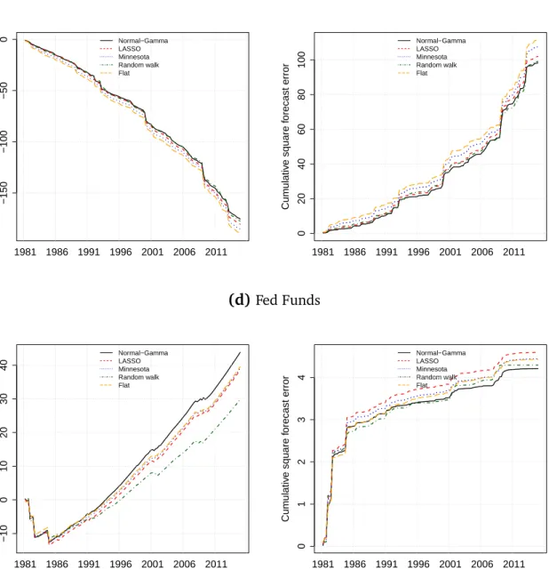
To investigate this issue further, Fig. 3 evaluates the forecast performance over time for the one-step-ahead forecast horizon. The left panel depicts the evolution of the cumulative LPS over time while the right panel shows the evolution of the cumu-lative sum of squared forecast errors over time. Here, the priors yield a very similar forecasting performance with the quality of forecasts deteriorating during times of well-known episodes of economic crises. For example, for all variables a considerable decrease in the LPS score is witnessed around 2008, mirrored in a sharp increase in the RMSE. Forecast performance also deteriorates around 1990, a period that was characterized by the first Gulf war and a related oil price shock, and around 2000, a time frame that featured the burst of the dot-com bubble. While the Normal-Gamma prior ranges always among the top-performing priors throughout the hold-out sam-ple, it does a particularly good job in forecasting the Federal Funds rate and inflation.
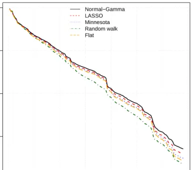
Last, Fig. 4 shows the LPS evaluated for the joint predictive likelihood for the
four variables at the one-step-ahead forecast horizon. This joint predictive likelihood
is obtained by integrating out the other variables in yt not further investigated in
the present forecasting comparison.6 Here it becomes evident that the naive model
and the flat prior VAR perform worst, and the difference in LPS scores relative to the Normal-Gamma prior even widens from the beginning of the 1990s. That is, the benefits of the Normal-Gamma prior are particularly evident in the most recent period of the hold-out sample where forecast gains of the Normal-Gamma prior are even more pronounced compared to its strongest competitor, the LASSO prior.
Cumulative log predictive likelihood Cumulative sum of squared forecast errors (a)GDP −150 −100 −50 0 Cum ulativ e log predictiv e score Normal−Gamma LASSO Minnesota Random walk Flat 1981 1986 1991 1996 2001 2006 2011 0 20 40 60 Cum ulativ e square f orecast error Normal−Gamma LASSO Minnesota Random walk Flat 1981 1986 1991 1996 2001 2006 2011 (b)Inflation −40 −30 −20 −10 0 Cum ulativ e log predictiv e score Normal−Gamma LASSO Minnesota Random walk Flat 1981 1986 1991 1996 2001 2006 2011 0 2 4 6 8 10 12 Cum ulativ e square f orecast error Normal−Gamma LASSO Minnesota Random walk Flat 1981 1986 1991 1996 2001 2006 2011
Notes: Cumulative log predictive scores and cumulative sum of squared forecast errors over the hold-out sample (1981Q1 to 2014Q4). Results based on 5,000 posterior draws out of a chain of 15,000 posterior draws.
Cumulative log predictive likelihood Cumulative sum of squared forecast errors (c)Wages −150 −100 −50 0 Cum ulativ e log predictiv e score Normal−Gamma LASSO Minnesota Random walk Flat 1981 1986 1991 1996 2001 2006 2011 0 20 40 60 80 100 Cum ulativ e square f orecast error Normal−Gamma LASSO Minnesota Random walk Flat 1981 1986 1991 1996 2001 2006 2011 (d)Fed Funds −10 0 10 20 30 40 Cum ulativ e log predictiv e score Normal−Gamma LASSO Minnesota Random walk Flat 1981 1986 1991 1996 2001 2006 2011 0 1 2 3 4 Cum ulativ e square f orecast error Normal−Gamma LASSO Minnesota Random walk Flat 1981 1986 1991 1996 2001 2006 2011
Notes: Cumulative log predictive scores and cumulative sum of squared forecast errors over the hold-out sample (1981Q1 to 2014Q4). Results based on 5,000 posterior draws out of a chain of 15,000 posterior draws.
Fig. 3: Evolution of the one-step ahead cumulative predictive likelihood along with the corresponding cumulative sum of squared forecast errors: (a) GDP, (b) real wages, (c) consumer price inflation, and (d) federal funds rate.
−300 −200 −100 0 Cum ulativ e log predictiv e score Normal−Gamma LASSO Minnesota Random walk Flat 1981 1986 1991 1996 2001 2006 2011
Notes: Cumulative log joint predictive scores over the hold-out sample (1981Q1 to 2014Q4). Re-sults based on 5,000 posterior draws out of a chain of 15,000 posterior draws.
Fig. 4: Evolution of the one-step ahead cumulative joint predictive likelihood. 4.3 Dynamic responses of selected macroeconomic quantities
In this subsection we examine the response generated by the NG-VAR and a flat prior VAR to a monetary policy shock.
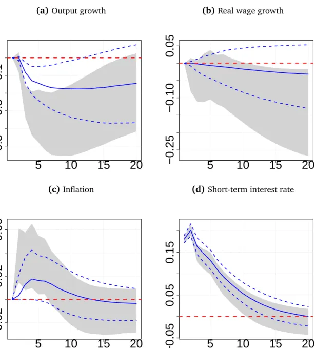
Figure 5 depicts the responses of output, real wages, inflation and interest rates
to a one standard deviation monetary policy shock in the US. We use a recursive ordering with the short-term interest rate ordered last (the ordering is consumption, investment, real GDP growth, hours worked, inflation, real wages and the short-term
interest rate). Similar toFig. 2, the dashed blue lines depict 16th and 84th credible
intervals and the blue solid line is the posterior median of impulse responses of the NG-VAR. Moreover, the gray shaded areas again represent the 16th and 84th credible sets of impulse responses for a flat prior VAR.
Figure 5(a) displays the dynamic response of output growth to a contractionary
monetary policy shock. In line with the literature, real GDP growth decreases signifi-cantly in the medium run, with output reactions turning insignificant after around 12 quarters. Comparing the responses of the flat prior VAR, the NG-VAR generates more
(a)Output growth
5
10
15
20
−0.5
−0.3
−0.1
(b)Real wage growth
5
10
15
20
−0.25
−0.10
0.05
(c)Inflation5
10
15
20
−0.02
0.02
0.06
(d) Short-term interest rate
5
10
15
20
−0.05
0.05
0.15
Notes: The dashed blue lines represent the 16th and 84th credible sets and the blue line denotes the median of impulse responses from the NG-VAR. The gray shaded represent the 16th and 84th credible interval of impulse responses of a flat prior VAR.
Fig. 5: Impulse responses of selected macroeconomic variables to a monetary policy shock
modest effects on output growth. In addition, the shape of the impulses suggests that the effect of monetary policy is somewhat longer lasting under a flat prior.
Turning to real wage growth, shown in Fig. 5(b), we find that under a flat prior VAR model, real wages tend to decline significantly and persistently so. By contrast, responses of the NG-VAR indicate that the effect on wage growth is close to zero and estimated with a lot of uncertainty. Modest reactions of wage growth to a monetary
policy shock have been found inChristiano et al.(2005) and are consistent with New
Keynesian models of the business cycle that incorporate nominal rigidities into the modeling framework.
Finally, Figs. 5 (c) and (d) present the responses of inflation and short-term
in-terest rates. Note that while both specifications produce a price puzzle, i.e., inflation acceleration in response to contractionary monetary policy, median effects are much smaller based on the NG-VAR. Moreover and looking at the credible sets, the positive response of inflation is barely significant under the NG-VAR but highly so under the flat prior VAR. The responses of interest rates appear to be quite similar for both pri-ors, with the effect on interest rates being slightly more persistent under the NG-VAR. 5 Extending the basic Normal-Gamma prior
In this section we relax the assumption of a single global shrinkage parameterλψ and
introduce three modifications of the Normal-Gamma prior setup of Section 2. 5.1 Three modifications
We modify the Normal-Gamma prior by introducing the following generalizations 1. The first modification introduces equation-specific shrinkage parameters and
thus shrinks each row of A towards a zero matrix. This implies that distinct
parametersλψj andϑψj forj = 1, . . . , mare introduced to effectively allow for a different degree of sparsity across equations. This is predicated by the fact that some variables may be better represented by small-scale models.
2. In the second modification we introduce k shrinkage parameters λψi, ϑψi (i =
1, . . . , k)that shrink certain columns ofAtowards zero. Thus, if the researcher
believes that some elements ofxttend to be unimportant to predictyt, then the
corresponding columns ofAare pushed towards a zero vector.
3. Finally, we introducemadditional shrinkage parameters that shrink the columns
related toalllagged endogenous variables. Hence, if we exclude theith element
of yt−1, yit−1, we also exclude all plags of yit. This implies that if variable iin yt−1 appears to be irrelevant to predictyt, we do not only excludeyit−1 but also
The first two modifications of the Normal-Gamma prior have recently been applied inKastner(2016) in a factor stochastic volatility framework to obtain a sparse repre-sentation of the factor loadings.
The conditional posterior distributions outlined in Section 2.3 still apply with some minor modifications that are derived in a straightforward fashion. Note that
apart from obvious alterations to the posterior moments inEq. (2.12)and Eq. (2.14)
to account for different λψis, the product and sum in Eqs. (2.16) and (2.17) have
to be modified to include only the relevant ψjs. More information can be found in
Appendix A.
5.2 Forecasting evidence
In this subsection we assess whether these modifications pay off in terms of forecast accuracy. Apart from the introduced generalizations, the setting is exactly the same as the one presented in Subsection 4.2.
Table3displays the results across the different alterations of the Normal-Gamma
prior. Normal-Gamma again presents the results of our baseline Normal-Gamma prior with a single global shrinkage parameter while Normal-Gamma row-wise is the model based on equation-specific shrinkage parameters and column-wise presents the
find-ings based on shrinking each column of Xt towards zero with a distinct
parame-ters. Finally, block-wise corresponds to the specification that introducesmadditional
shrinkage parameters to effectively exclude certain lagged elements of yt entirely
fromXt.
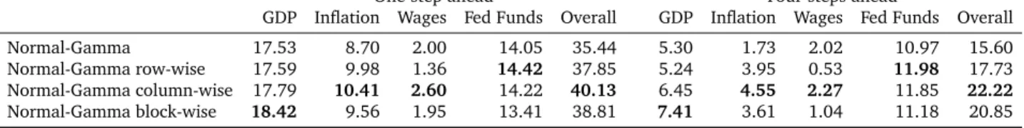
Our findings suggest that the performance of the baseline prior can still be im-proved considerably in terms of density predictions. The column-wise specification, which constitutes the most flexible prior framework along the variants discussed, ex-hibits a strong forecasting performance across all variables and for both time horizons considered. Note that the single best performing specification for GDP predictions proves to be the block-wise specification, improving upon the second strongest spec-ification considerably. For all other variables, the block-wise specspec-ification tends to perform slightly worse.
Sum of log predictive scores (LPS) relative to the random walk
One-step ahead Four-steps ahead
GDP Inflation Wages Fed Funds Overall GDP Inflation Wages Fed Funds Overall Normal-Gamma 17.53 8.70 2.00 14.05 35.44 5.30 1.73 2.02 10.97 15.60 Normal-Gamma row-wise 17.59 9.98 1.36 14.42 37.85 5.24 3.95 0.53 11.98 17.73 Normal-Gamma column-wise 17.79 10.41 2.60 14.22 40.13 6.45 4.55 2.27 11.85 22.22
Normal-Gamma block-wise 18.42 9.56 1.95 13.41 38.81 7.41 3.61 1.04 11.18 20.85 Average root mean square forecast errors (RMSE) relative to the random walk
One-step ahead Four-steps ahead GDP Inflation Wages Fed Funds GDP Inflation Wages Fed Funds
Normal-Gamma 0.93 1.11 1.00 0.99 0.93 1.06 0.98 0.88
Normal-Gamma row-wise 0.93 1.11 1.00 0.99 0.93 1.06 0.98 0.88
Normal-Gamma column-wise 0.94 1.11 1.00 0.99 0.92 1.06 0.98 0.88
Normal-Gamma block-wise 0.94 1.13 1.00 1.00 0.93 1.07 0.99 0.89
Notes:NG stands for a vector autoregressive model coupled with a Normal-Gamma prior, Normal-Gamma row-wise is the alteration of the Normal-Gamma prior that estimates an equation-specific shrinkage hyperparameter, Normal-Gamma column-wise introduces additional shrinkage parameters for each column ofXtand Normal-Gamma block-wise refers to the prior that includes certain lagged elements ofytand the lags thereof. GDP refers to real GDP per capita growth, Wages to real per capita wage growth, inflation to CPI inflation and Fed Funds to the federal funds rate. The bold figures indicate the best performing model for a given variable and time horizon.
Table 3: Out-of-sample performance of different variants of the NG-VAR relative to the random walk model in terms of the sum of log predictive scores (LPS) and the root mean square error (RMSE): 1981:Q1 to 2014:Q4
For some variables, we see that the additional flexibility slightly improves density predictions. This finding, however, does not carry over to point predictions.
Inspec-tion of the lower part of Table3reveals that the accuracy of point forecasts is basically
the same across the different variants of the Normal-Gamma prior, suggesting that ad-ditional shrinkage parameters exhibit performance-enhancing effects on higher order moments of the predictive density, as opposed to mere mean predictions.
6 Closing remarks
In this paper we generalize the shrinkage prior put forward inGriffin et al.(2010) to
the VAR case. This framework induces global shrinkage by pushing the full coefficient matrix of the model towards zero a priori. Imposing a set of Gamma priors results into fat-tailed prior on the coefficients. This ensures that the global shrinkage factor does not push coefficients too strongly towards zero and allows for a great deal of flexibility.
We evaluate the merits of the Normal-Gamma prior for the VAR case by means of a simple simulation exercise and an out-of-sample forecast competition. Our findings show that the precision of the estimates for the autoregressive coefficients and the covariances originating from the NG-VAR systematically outperform estimates stem-ming from competing models like a typical Bayesian VAR with a Minnesota prior and a flat prior VAR. This holds also true in case the quantity of interest are impulse
re-sponse functions. Here, the NG-VAR produces tighter credible sets than a flat prior VAR and the median response is always close to the simulated values. In some cases, the VAR with a diffuse prior even indicates significant non-zero responses albeit the simulated response is zero. This is not the case when using the NG-VAR.
In a real data application, we examine the usefulness of the NG-VAR by evaluating forecasts and impulse response functions for a medium-VAR with US data put forth in
Smets and Wouters(2003) and extended inGeweke and Amisano(2012). The results reveal the NG-VAR forecasts outperforming its competitors systematically at the one-step-ahead forecast horizon and in almost all cases four steps ahead. Looking at the responses to a contractionary monetary policy shock, we find negative and tightly estimated effects on output growth, and a rather persistent rise in the short-term interest rate. Responses of inflation and real wage growth are accompanied by wide credible sets. These results are well in line with existing literature and demonstrate the usefulness of the NG-VAR approach not only in terms of forecasting but also for structural analysis.
Finally, we introduce three extensions of the Normal-Gamma prior adding more flexibility to the baseline specification. Our findings suggest that the modified Normal-Gamma priors excel in density forecasts, while improvements in point predictions are modest.
References
Ba´nbura M, Giannone D and Reichlin L (2010) Large Bayesian vector
auto-regressions. Journal of Applied Econometrics25(1), 71–92
Bhattacharya A, Pati D, Pillai NS and Dunson DB (2015) Dirichlet–Laplace priors for
optimal shrinkage.Journal of the American Statistical Association110(512), 1479–
1490
Carriero A, Clark TE and Marcellino M (2015) Bayesian VARs: specification choices
and forecast accuracy. Journal of Applied Econometrics30(1), 46–73
Carriero A, Kapetanios G and Marcellino M (2009) Forecasting exchange rates with a
large Bayesian VAR. International Journal of Forecasting25(2), 400–417
Carriero A, Kapetanios G and Marcellino M (2012) Forecasting government bond
yields with large Bayesian vector autoregressions. Journal of Banking & Finance
36(7), 2026–2047
Christiano LJ, Eichenbaum M and Evans CL (2005) Nominal rigidities and the
dy-namic effects of a shock to monetary policy. Journal of political Economy 113(1),
1–45
Doan TR, Litterman BR and Sims CA (1984) Forecasting and conditional projection
using realistic prior distributions. Econometric Reviews3(1), 1–100
Gefang D (2014) Bayesian doubly adaptive elastic-net Lasso for VAR shrinkage.
In-ternational Journal of Forecasting30(1), 1–11
George EI and McCulloch RE (1993) Variable selection via Gibbs sampling. Journal
of the American Statistical Association88(423), 881–889
George EI, Sun D and Ni S (2008) Bayesian stochastic search for VAR model
restric-tions. Journal of Econometrics142(1), 553–580
Geweke J and Amisano G (2010) Comparing and evaluating Bayesian predictive
dis-tributions of asset returns. International Journal of Forecasting26(2), 216–230
Geweke J and Amisano G (2012) Prediction with misspecified models. The American
Economic Review102(3), 482–486
Giannone D, Lenza M, Momferatou D and Onorante L (2014) Short-term inflation
projections: A Bayesian vector autoregressive approach. International journal of
forecasting30(3), 635–644
Giannone D, Lenza M and Primiceri GE (2015) Prior selection for vector
autoregres-sions. Review of Economics and Statistics97(2), 436–451
Griffin JE, Brown PJ et al. (2010) Inference with normal-gamma prior distributions
in regression problems. Bayesian Analysis5(1), 171–188
Kadiyala KR, Karlsson S et al. (1997) Numerical Methods for Estimation and Inference
in Bayesian VAR-Models. Journal of Applied Econometrics12(2), 99–132
Karlsson S (2013) Forecasting with Bayesian vector autoregressions. Handbook of
Economic Forecasting2, 791–897
Dy-namic Covariance Estimation in High-Dimensional Time Series. Mimeo
Koop GM (2013) Forecasting with medium and large Bayesian VARs. Journal of
Ap-plied Econometrics28(2), 177–203
Litterman R (1979) Techniques of forecasting using vector autoregressions. Technical report, Federal Reserve Bank of Minneapolis
Litterman R (1986) Forecasting with Bayesian vector autoregressions – Five years of
experience. Journal of Business and Economic Statistics4(1), 25–38
Park T and Casella G (2008) The Bayesian Lasso. Journal of the American Statistical
Association103(482), 681–686
Polson NG and Scott JG (2010) Shrink globally, act locally: Sparse Bayesian
regular-ization and prediction. Bayesian Statistics9, 501–538
Pourahmadi M (1999) Joint mean-covariance models with applications to
longitudi-nal data: Unconstrained parameterisation. Biometrika86(3), 677–690
Sims CA (1993) A nine-variable probabilistic macroeconomic forecasting model. In
Business Cycles, Indicators and Forecasting. University of Chicago Press, 179–212
Sims CA and Zha T (1998) Bayesian methods for dynamic multivariate models.
In-ternational Economic Review39(4), 949–968
Smets F and Wouters R (2003) An estimated dynamic stochastic general equilibrium
model of the euro area. Journal of the European economic association1(5), 1123–
1175
Smith M and Kohn R (2002) Parsimonious covariance matrix estimation for
Appendix A Derivations
In this section we derive the relevant posterior quantities for the baseline Normal-Gamma prior and the extensions presented in Section 5.
A.1 Derivations related to the baseline Normal-Gamma prior
To deriveEq. (2.14), note that due to the hierarchical nature of the model, the
con-ditional posterior ofψi is independent from the data. Combining the likelihood with
the prior yields
p(ψi|ϑψ, λ 2 ψ, αi)∝ψ −1/2 α exp −α 2 i 2ψi ×ψ(ϑψ−1) i exp −ϑψλ 2 ψψi 2 (A.1) ∝ψ(ϑψ−0.5)−1 i exp −(α 2 i ψi +ϑψλ2ψψi)/2 (A.2) where we exploit the scaling property of the Gamma distribution to rewrite the prior inEq. (2.5)as
αi|ψi ∼ N(0, ψi), ψi ∼ G(ϑψ, ϑψλ2ψ/2). (A.3)
Equation (A.2) is the kernel of the GIG distribution described in Eq. (2.14).
Equation (2.17) is derived by combining the Gamma likelihood with the prior and
simplifying yields p(λψ|ψ, ϑψ)∝λ (kϑψ+cψ0)−1 ψ ×exp (cψ1+ ϑψ 2 mk j=1 ψj)λψ , (A.4)
which is the kernel of a Gamma density with shape parameter equal tokϑψ+cψ0 and
rate parameter given bycψ1+
ϑψ
2 mk
j=1ψj.
The derivation ofEq. (2.24)closely resembles the derivation ofEq. (2.14). Finally,
the derivation ofEq. (2.26)is analogous to the derivation ofEq. (2.17).
A.2 Derivations related to the three extensions in Section 5
As noted in Section 5, the relevant conditional posterior distributions outlined in Section 2 can still be used with only minor alterations.
The generalization ofEq. (2.12)associated with the first modification (row-wise) is given by [Vα]ii= 2/λ2 ψ1ψi ifi∈ A (1) 1 ={1, . . . , k} 2/λ2 ψ2ψi ifi∈ A (1) 2 ={k+ 1, . . . ,2k} .. . 2/λ2 ψmψi ifi∈ A (1) m ={(m−1)k+ 1, . . . , mk}. (A.5)
For the column-wise specification, the corresponding variant ofEq. (2.12)is
[Vα]ii= 2/λ2 ψ1ψi ifi∈ A (2) 1 ={1,1 +k, . . . ,1 + (m−1)k} 2/λ2 ψ2ψi ifi∈ A (2) 2 ={2,2 +k, . . . ,2 + (m−1)k} .. . 2/λ2 ψkψi ifi∈ A (2) k ={k,2k, . . . , mk}. (A.6)
Finally, for the third variant we specify the prior variance such that
[Vα]ii= 2/λ2 ψ1ψi ifi∈ A (3) 1 ={1,1 +m,1 + 2m, . . . ,1 + (p−1)m} 2/λ2 ψ2ψi ifi∈ A (3) 2 ={2,2 +m,2 + 2m, . . . ,2 + (p−1)m} .. . 2/λ2ψmψi ifi∈ A (3) m ={m,2m, . . . , k}. (A.7)
Under Eqs. (A.5) to (A.7), the conditional posterior ofAremains the same.
The modified counterpart ofEq. (2.14)is given by
ψi|ϑψ, λ2ψ, αi ∼ GIG(ϑψ − 1 2, ϑψjλ 2 ψj, α 2 i) (A.8)
where we choose the appropriate parametersλψj andϑψjifibelongs to the
appropri-ate setA(sn).
The acceptance probability in2.16is modified to take into account that we sample
differentϑψj, min 1,p(ϑ ∗ ψj) p(ϑψj) (ϑ∗ψjλ 2 ψj/2) kϑ∗ ψj (ϑψjλ2ψj/2) kϑψj Γ(ϑ∗ψj) Γ(ϑψj) j∈A(sn) ψj ϑ∗ψj−ϑψj , (A.9) for variantsn = 1,2,3.
Similarly, we adaptEq. (2.17)as λ2ψj|ϑψj,ψ∼ G cψ0+ϑψjq (n) j , cψ0+ϑψ/2 j∈A(sn) ψj . (A.10)
Here, we letqj(n)= #(A(sn))denote the cardinality ofA (n) s .
Steps 4 and 5 of the MCMC algorithm presented in Section 2 have to be modified
to draw distinctλ2
ψj and ϑψj for each variant of the prior. These steps are