UNIVERSITY OF LYON DOCTORAL SCHOOL OF COMPUTER SCIENCES AND MATHEMATICS P H D T H E S I S. Specialty : Computer Science. Author

(1)

UNIVERSITY OF LYON

DOCTORAL SCHOOL OF COMPUTER SCIENCES

AND MATHEMATICS

P H D T H E S I S

Specialty : Computer Science

Author

S´ergio

Rodrigues de Morais

on November 16, 2009

Bayesian Network Structure Learning

with Applications in Feature Selection

Jury :

Reviewers : Pr. Philippe Leray - University of Nantes

Pr. Florence D’Alch´e-Buc - University of Evry-Val d’Essonne

Examinators : PhD. DavidGarcia - Pˆole Europ´een de Plasturgie PhD. EmmanuelMazer - GRAVIR Laboratory

Thesis Advisors : Pr. Alexandre Aussem - UCBL, University of Lyon Pr. Jo¨elFavrel - INSA, University of Lyon

(2)

I would like to dedicate this thesis to my loving parents, my brother and my sister ...

(3)

Acknowledgements

I will forever be thankful to my PhD advisor, Professor Alexandre Aussem. His scientific advice and insightful discussions were essential for this work. Alexandre has been supportive and has given me the freedom to pursue my own proposals without objection. The most important, he has believed in me and given me opportunities that nobody would have... Thanks Alex!

I also thank my collaborators, specially David Garcia and Philippe Le Bot. Their enthusiasm and professionalism are contagious. Their questions and advices were of great significance for my work. Thank you for your patience and help.

I am also very grateful to Jo¨el Favrel, who was one of my two PhD advisors. He was a role model for a scientist, mentor, and teacher. Thank you for your advices and kindness.

I would like to acknowledge the ”Ligue contre le Cancer, Comité du Rhône, France”, which supported the work of chapter 6. The dataset used in this chapter was kindly supplied by the International Agency for Research on Cancer (Lyon - France). I would also like to acknowl-edge Sophie Rome and the ”Institut des Sciences Complexes” (Lyon - France), who supported and helped in the work presented in chap-ter 7. Finally, I would like to acknowledge André Tchernof and the

”Centre de recherche en endocrinologie moléculaire et oncologique et génomique humaine” (Québec - Canada), who supported and gave great assistance to the work presented in chapter 8.

(4)

Abstract

The study developed in this thesis focuses on constraint-based meth-ods for identifying the Bayesian networks structure from data. Novel algorithms and approaches are proposed with the aim of improving Bayesian network structure learning with applications to feature sub-set selection, probabilistic classification in the presence of missing val-ues and detection of the mechanism of missing data. Extensive empir-ical experiments were carried out on synthetic and real-world datasets in order to compare the methods proposed in this thesis with other state-of-the-art methods. The applications presented include extract-ing the relevant risk factors that are statistically associated with the Nasopharyngeal carcinoma, a robust analysis of type 2 diabetes from a dataset consisting of 22,283 genes and only 143 samples and a graph-ical representation of the statistgraph-ical dependencies between 34 clingraph-ical variables among 150 obese women with various degrees of obesity in order to better understand the pathophysiology of visceral obesity and provide guidance for its clinical management.

Keywords: Bayesian networks, feature subset selection, missing data mechanism, classification, pattern recognition.

(5)

Contents

1 Introduction 1 1.1 An Overview . . . 1 1.2 Author’s Contributions . . . 4 1.3 Applications . . . 5 1.4 Outline . . . 6

2 Background about Bayesian networks and structure learning 8 2.1 Introduction . . . 8

2.2 Some principles of Bayesian networks . . . 10

2.2.1 Markov condition and d-separation . . . 11

2.2.2 Markov equivalence . . . 15

2.2.3 Embedded Faithfulness . . . 17

2.2.4 Markov blankets and boundaries . . . 18

2.3 Constraint-based structure learning . . . 19

2.3.1 Soundness of constraint-based algorithms . . . 19

2.3.2 G likelihood-ratio conditional independence test . . . 22

2.3.3 Fisher’s Z test . . . 23

2.4 Existence of a perfect map . . . 25

2.4.1 Conditional independence models . . . 26

2.4.2 Graphical independence models . . . 27

2.4.3 Algebraic independence models . . . 28

(6)

STRUCTURE LEARNING

31

3 Local Bayesian network structure search 32

3.1 Introduction . . . 32

3.2 Preliminaries . . . 34

3.2.1 Conditional Independence Test . . . 35

3.2.2 Pitfalls and related work . . . 36

3.3 HPC: the Hybrid Parents and Children algorithm . . . 41

3.4 HPC correctness under faithfulness condition . . . 46

3.5 Experimental validation . . . 49

3.5.1 Accuracy . . . 50

3.5.2 Scalability . . . 51

3.6 MBOR: an extension of HPC for feature selection . . . 53

3.7 Discussion and conclusions . . . 56

4 Conservative feature selection with missing data 60 4.1 Introduction . . . 60

4.2 Preliminaries . . . 62

4.2.1 Dealing with missing values . . . 62

4.2.2 Deletion process . . . 63

4.3 A conservative Markov blanket . . . 64

4.4 A conservative independence test . . . 65

4.4.1 Extension to conditional G-tests . . . 68

4.5 Experimental evaluation . . . 68

4.5.1 Limits of the conservative test . . . 70

4.5.2 Ramoni and Sebastiani’s benchmark . . . 71

4.5.2.1 Procedure used to remove data . . . 73

4.5.3 Results of the empirical experiments . . . 76

4.6 Discussion and Conclusions . . . 76

5 Exploiting data missingness through Bayesian network modeling 78 5.1 Introduction . . . 78

5.2 Related work . . . 80

(7)

APPLICATIONS

94

6 Analysis of nasopharyngeal carcinoma risk factors 95 6.1 Introduction . . . 95

6.2 Graph construction with inclusion of domain knowledge . . . 97

6.3 Graph-based analysis and related work . . . 98

6.4 Predictive performance . . . 101

6.5 Model calibration . . . 103

6.6 Detection of the missing mechanisms . . . 104

7 Robust gene selection from microarray data 112 7.1 Introduction . . . 112

7.2 Robust feature subset selection . . . 113

7.3 Ensemble FSS by consensus ranking . . . 114

7.4 Experiments . . . 115

7.4.1 Robustness versus classification accuracy . . . 115

7.4.2 Ensemble FSS technique on Diabetes data . . . 116

8 Analysis of lifestyle and metabolic predictors of visceral obesity with Bayesian networks 122 8.1 Introduction . . . 122

8.2 Simulation experiments withHPC . . . 124

8.3 Results on biological data . . . 125

(8)

List of Figures

2.1 Toy example of causal network presented in the WCCI2008 Causation and

Prediction Challenge.. . . 9

2.2 Three Markov equivalent DAGs. There are no other DAGs Markov equivalent to them. . . 15

2.3 The marginal distribution of V, S, L and F cannot satisfy the faithfulness condition with any DAG. . . 18

3.1 Toy problem about PC learning: 6 ∃Z∈PCT, so that,X ⊥GT|Z. . . 38

3.2 Divide-and-conquer algorithms can be lessdata-efficient than incremental al-gorithms. . . 40

3.3 HPC empirical evaluation in terms of scalability.. . . 51

3.4 HPC empirical evaluation in terms of Euclidean distance from perfect preci-sion and recall.. . . 57

3.5 HPC empirical evaluation in terms of the number of false positives. . . 58

3.6 HPC empirical evaluation in terms of the number of false negatives. . . 59

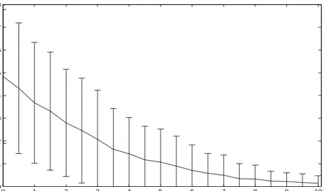
4.1 GreedyGmax’s p-value as a function of the ratio of missing data. . . 70

4.2 Subgraph taken from the benchmark ALARM displaying the MB of the vari-ableSHUNT. . . 72

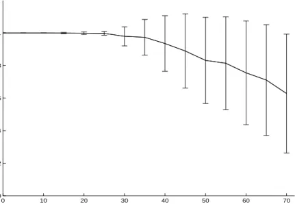
4.3 GreedyGmax’s p-value as a function of the ratio of missing data when testing on variables of the benchmark ALARM. . . 73

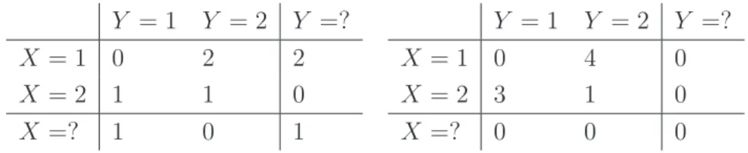
4.4 Original BN benchmark used by [Ramoni & Sebastiani (2001)]. . . 73

4.5 MCAR made from the original BN benchmark used by [Ramoni & Sebastiani (2001)]. . . 74

(10)

LIST OF FIGURES

4.6 MAR made from the original BN benchmark used by [Ramoni & Sebastiani

(2001)]. . . 75

4.7 NMAR (IM) made from the original BN benchmark used by [Ramoni & Se-bastiani (2001)]. . . 75

5.1 Toy examples of missing completely at random (MCAR). . . 79

5.2 Toy examples of missing at random (MAR). . . 80

5.3 Toy examples of not missing at random (NMAR/IM). . . 80

5.4 Probability tables used to vary the missing data ratio of the DAG shown in Figure 5.3 . . . 83

5.5 Average accuracy in detecting the mechanism NMAR (IM) of toy problem shown in Figure 5.3. . . 84

5.6 Graphical representation of the MCAR, MAR and NMAR (IM) used for em-pirical experiments. . . 88

5.7 Bayesian network used for generating data from the congressional voting records dataset. . . 90

5.8 Empirical evaluation ofGMB on a congressional voting reports dataset. . . . 91

5.9 Empirical evaluation ofGMB for MCAR, MAR and IM (NMAR). . . 93

6.1 Local BN graph skeleton around variable NPC. . . 107

6.2 Local PDAG of Figure 6.1 . . . 108

6.3 The ROC curves obtained by 10-fold cross-validation with a Naive Bayes clas-sifier. . . 110

6.4 Model calibration. Top: Markov boundary. Bottom: all variables.. . . 110

6.5 NPC graph with dummy missingness variables shown in dotted line. . . 111

7.1 Robustness vs MB size for the benchmarksGenes andPigs . . . 119

7.2 Comparative accuracy for the benchmarksGenes and Pigs. . . 120

7.3 MBOR outputs for a microarray data . . . 121

8.1 Bootstrap-based validation for the algorithmHPC on datasets from the bench-markINSULIN. . . 125

8.2 BN learned from 34 risk factors related to lifestyle, adiposity, body fat distri-bution, blood lipid profile and adipocyte sizes. . . 132

(11)

Chapter 1

Introduction

1.1

An Overview

A Bayesian networks (BN) is a graphical structure for representing the probabilis-tic relationships among a large number of features (or variables 1_{) and for doing} probabilistic inference with those features. The graphical nature of Bayesian net-works gives a very intuitive grasp of the relationships among the features. For example, a Bayesian network could represent the probabilistic relationships be-tween diseases and symptoms. Given symptoms, the network can be used to com-pute the probabilities of the presence of various diseases. Bayesian networks are used for modeling knowledge in computational biology and bioinformatics (gene regulatory networks, protein structure, gene expression analysis), medicine, docu-ment classification, information retrieval, image processing, data fusion, decision support systems, engineering, gaming and law. The term ”Bayesian networks” was coined by Judea Pearl to emphasize three aspects [Pearl (1986)]:

1. The often subjective nature of the input information.

2. The reliance on Bayes’s conditioning as the basis for updating information. 3. The distinction between causal and evidential modes of reasoning, which underscores Thomas Bayes’ posthumously published paper of 1763 [Bayes (1763)].

(12)

1.1 An Overview

There are numerous representations available for data analysis, including rule bases, decision trees, and artificial neural networks; and there are many tech-niques for data analysis such as density estimation, classification, regression, and clustering. So what do Bayesian networks have to offer? There are at least three answers:

1. Bayesian networks can readily handle incomplete data sets. For example, consider a classification or regression problem where two of the explanatory or input variables are strongly anti-correlated. This correlation is not a problem for standard supervised learning techniques, provided all inputs are measured in every case. When one of the inputs is not observed, however, most models will produce an inaccurate prediction, because they do not encode the dependencies between the input variable. Bayesian networks offer a natural way to encode such dependencies.

2. Bayesian networks help in the process of learning about causal relation-ships. Learning about causal relationships are important for at least two reasons. The process is useful when we are trying to gain understanding about a problem domain, for example, during exploratory data analysis. In addition, knowledge of causal relationships allows us to make predictions in the presence of interventions. For example, a marketing analyst may want to know whether or not it is worthwhile to increase exposure of a particular advertisement in order to increase the sales of a product. To answer this question, the analyst would like to determine whether or not the advertisement is a cause for increased sales, and to what degree. 3. Bayesian networks in conjunction with Bayesian statistical techniques

fa-cilitate the combination of domain knowledge and data. Anyone who has performed a real-world analysis knows the importance of prior or domain knowledge, especially when data is scarce or expensive. The fact that some commercial systems (i.e., expert systems) can be built from prior knowledge alone is a testament to the power of prior knowledge. Bayesian networks have a causal semantics that makes the encoding of causal prior knowl-edge particularly straightforward. In addition, Bayesian networks encode

(13)

1.1 An Overview

the strength of causal relationships with probabilities. Consequently, prior knowledge and data can be combined with well-studied techniques from Bayesian statistics.

Learning a Bayesian network from data requires identifying both the model structure G and the corresponding set of model parameter values. However, the study developed in this thesis focuses only on methods for identifying the Bayesian networks structure from data. The problem of learning the most probable a posteriori BN from data is worst-case NP-hard [Chickering (2002); Chickering

et al.(2004)] and the recent explosion of high dimensional datasets poses a serious challenge to existing BN structure learning algorithms. Two types of BN structure learning methods have been proposed so far: constraint-based (CB) and score-and-search methods. While score-score-and-search methods are efficient for learning the whole BN structure, the ability to scale up to hundreds of thousands of variables is a key advantage of CB methods over score-and-search methods. All the proposals of this thesis focus on improving constraint-based methods.

Several CB algorithms have been proposed recently for local BN structure learning [Fuet al.(2008); Nilsson et al. (2007a); Peña (2008); Peñaet al.(2007); Tsamardinos & Brown (2008); Tsamardinoset al.(2006)]. They search for condi-tional independence relationships among the variables on a dataset and construct a local structure around the target node without having to construct the whole BN first, hence their scalability. These algorithms are appropriate for situations where the sample size is large enough with respect to the network degree. That is, the number of parents and children (PC set) of each node in the network is relatively small with respect to the number of instances in the dataset. However, they are plagued with a severe problem: the number of false negatives increases swiftly as the size of the PC set increases. This well known problem is common to all CB methods and has led several authors to reduce, as much as possible, the size of the conditioning sets with a view to enhancing the data-efficiency of their methods [Fu et al.(2008); Peña et al.(2007); Tsamardinos et al.(2006)].

(14)

1.2 Author’s Contributions

1.2

Author’s Contributions

Main contributions to the field of constraint-based Bayesian network structure learning made by the author include:

1. A novel structure learning algorithm called Hybrid Parents and Children

(HPC) [Aussem et al. (2009b)]. HPC was proven to be correct under the faithfulness condition. Extensive empirical experiments were provided on public synthetic and real-world datasets of various sample sizes to assess

HPC’s accuracy and scalability. It was shown that significant improvements were obtained. In addition the number of calls to the independence test (and hence theeffective complexity) is onlyO(n1.09_{) in practice on the eight BN} benchmarks that we considered and O(n1.21_{) on a real drug design dataset} characterized by almost 140,000 features.

2. An extension of HPC designed for the specific aim of features selection for probabilistic classification. Such extension is calledMBOR and was already applied in [Aussemet al.(2009c); de Morais & Aussem (2008a,b)] with very promising results after extensive empirical experiments on synthetic and real-world datasets. MBOR searches the Markov boundary of a target as a solution for the problem of features selection and was shown to scale up to hundreds of thousands of variables. As the algorithm HPC, MBOR was also proven to be correct under the faithfulness condition.

3. A novel conservative features selection method for handling incomplete datasets [Aussem & de Morais (2008)]. The method is conservative in the sense that it selects the minimal subset of features that renders the rest of the features independent of the target (the class variable) without making any assumption about the mechanism of missing data. The idea is that, when no information about the pattern of missing data is available, an in-complete dataset contains the set of all possible estimates. This conservative test addresses the main shortcoming of CB methods with missing data: the difficulty of performing an independence test when some entries are missing without making any assumption about the missing data mechanism.

(15)

1.3 Applications

4. A new graphical approach for exploiting data missingness in Bayesian net-work modeling [de Morais & Aussem (2009a)]. The novel approach makes use of Bayesian networks for explicitly representing the information about the absence of data. This work focused on two different, but not inde-pendent aims: first, to help detecting the missing data mechanisms, and second, to improve accuracy in classification when working with missing data. The missingness information is taken into account in the structure of the Bayesian network that will represent the joint probability distribution of all the variables, including new dummy variables that were artificially created for representing missingness.

1.3

Applications

The main applications of the methods presented in this thesis to real-world prob-lems made by the author include:

1. Application of the algorithm HPC for extracting the relevant risk factors that are statistically associated with the Nasopharyngeal Carcinoma (NPC) [Aussem et al. (2009a)]. Experiments for detecting the missing data mech-anisms present in this dataset were also carried out. The dataset was ob-tained from a case-control epidemiologic study performed by the Interna-tional Agency for Research on Cancer in the Maghreb (north Africa). It consists of 1289 subjects (664 cases of NPC and 625 controls) and 150 nominal variables. In this study, special emphasis is placed on integrating domain knowledge and statistical data analysis. Once the graph skeleton is constructed from data, it is afterwards directed by the domain expert ac-cording to his causal interpretation and additional latent variable are added to the graph for sake of clarity, coherence and conciseness. The graphical representation provides a statistical profile of the recruited population, and meanwhile help identifying the important risk factors involved in NPC. 2. Application of the algorithm MBOR on a microarray dataset in order to

provide a robust analysis of type 2 diabetes [Aussem et al. (2009c)]. The dataset used in this study consists of 22,283 genes and only 143 samples. It

(16)

1.4 Outline

was obtained in collaboration with INSERM U870/INRA 1235 laboratory and represents a compilation of different microarray data published during the last five years on the skeletal muscle from patients suffering from type 2 diabetes, obesity or from healthy subjects. Multiple runs of MBOR on re-samples of the microarray data are combined, using ensemble techniques, to yield more robust results. Genes were aggregated into a consensus genes rank and the top ranked features were analyzed by biologists. It was shown that the findings presented in this study are in nice agreement with the genes that were associated with an increased risk of diabetes in the recent medical literature.

3. The algorithm HPC was applied for representing the statistical dependen-cies between 34 clinical variables among 150 obese women with various degrees of obesity. Features affecting obesity are of high current interest. Clinical data, such as patient history, lifestyle parameters and basic or even more elaborate laboratory analyses (e.g., adiposity, body fat distribution, blood lipid profile and adipocyte sizes) form a complex set of inter-related variables that may help better understand the pathophysiology of visceral obesity and provide guidance for its clinical management. In the work presented in this chapter bootstrapping method was used to generate more robust network structures. Statistical significance of edge strengths are eval-uated using this approach. If an edge has a confidence above the threshold, it is included in the consensus network. This study made thorough use of integration of physiological expertise into the graph structure.

1.4

Outline

This thesis is divided into 9 chapters. A great effort was made in order to provide self contain chapters. For this reason some redundant information can be seen from one chapter to another. However, the brief background provided in chapter 2 is necessary for everyone who is not familiar to Bayesian networks. Chapter 2 provides the important background about the principal concepts of Bayesian networks and constraint-based learning. In chapter 3, the algorithms HPC and

(17)

1.4 Outline

MBOR are introduced. Furthermore, this chapter also presents the parallel ap-proach for both algorithms HPC and MBOR and a thorough discussion about the main problems that plague CB Bayesian networks structure learning, includ-ing the problem of almost-deterministic relationships among variables. Chapter 4 introduces a novel conservative features selection method for handling incomplete datasets. A different approach is presented in chapter 5 which exploits data miss-ingness in Bayesian network modeling. The last chapters of this thesis contain several applications to real-world problems. In chapter 6 the algorithm HPC was applied for extracting the relevant risk factors that are statistically associated with the Nasopharyngeal Carcinoma. In chapter 7 the algorithm MBOR (Chap-ter 3) is applied on a microarray dataset in order to provide a robust analysis of type 2 diabetes. A graphical representation for helping identifying the most important predictors of visceral obesity was achieved in chapter 8 by applying the algorithm HPC on a dataset containing 34 clinical variables among 150 obese women with various degrees of obesity. Finally, chapter 9 presents a summary and discusses future work.

(18)

Chapter 2

Background about Bayesian

networks and structure learning

2.1

Introduction

Bayesian networks (BN) are probabilistic graphical models that offer a coher-ent and intuitive represcoher-entation of uncertain domain knowledge. Formally, BN are directed acyclic graphs (DAG) modeling probabilistic conditional indepen-dences among variables. The graphical part of BN reflects the structure of a problem, while local interactions among neighboring variables are quantified by conditional probability distributions. One of the main advantages of BN over other artificial intelligence (AI) schemes for reasoning under uncertainty is that they readily combine expert judgment with knowledge extracted from the data within the probabilistic framework. Another advantage is that they represent graphically the (possibly causal) independence relationships that may exist in a very parsimonious manner [Brown & Tsamardinos (2008)]. Formally, a BN is a tuple < G, P >, where G =< U,E > is a directed acyclic graph with nodes representing the random variablesUandP a joint probability distribution onU. In addition, GandP must satisfy the Markov condition: every variable,Xi ∈U,

is independent of any subset of its non-descendant variables conditioned on the set of its parents, denoted by PaG_i.

The analysis of the Bayesian network structure can give very important in-formation for understanding a problem at hand. For instance, let us consider

(19)

2.1 Introduction

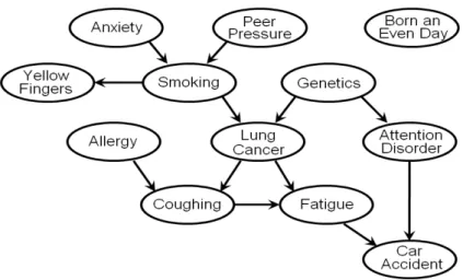
Figure 2.1: Toy example of causal network presented in the WCCI2008 Causation and Pre-diction Challenge.

the causal network presented in figure 2.1. This network was presented as a toy example of causal network in theWCCI2008 Causation and Prediction Challenge

[Guyon et al. (2008)]. When data is generated from a causal network, then such causal network very often coincides with the structure of a Bayesian network that represents the joint probability distribution of the variables in the problem. Clearly, the causal network of figure 2.1 is acyclic, therefore it is called a ”causal DAG”. However, such DAG must satisfy the Markov condition in order to be a Bayesian network. The concept of causality is something rather controversial, but when one consider that an effect is a future consequence of a past cause, then the Markov condition is observed from a causal DAG. It means that when the empirical data is generated from a causal DAG G by a stochastic process, then G and P satisfy the Markov condition. In other words, if the value of each variable Xi is chosen at random with some probability P(Xi|PaGi), based solely

on the values of PaG

i, then the overal distribution P of the generated instances

x1, x2, ..., xn and the DAG Gwill satisfy the Markov condition [Pearl (2000)].

A lot of information can be taken from the Bayesian network that coincides with the causal DAG presented in figure 2.1. For instance, it is clear that Smok-ing is directly associated with Lung Cancer. One can also see that even if Yellow Fingers is associated withLung Cancer it is not a direct association, but it passes

(20)

2.2 Some principles of Bayesian networks

through Smoking. It is clear thatBorn an Even Day has nothing to do withLung Cancer. Interestingly Car Accident could be even more predictive in relation to

Lung Cancer than Smoking because there are three information paths between

Lung Cancer and Car Accident. Nonetheless, for a physician it would be much more important to discover that Smoking has a direct impact to developingLung Cancer, than thatCar Accident is predictive. One can see thatAllergyis indepen-dent of Lung Cancer when there is no information about the values of the other variables, but when it is known that a patient is frequently Coughing, then the fact of knowing that the same patient has no Allergy can increase the probability of this patient having Lung Cancer... However, the structure of such a Bayesian network is not known beforehand when a dataset containing observational data is the only available piece of information. The Bayesian network structure search is the main aim of what is presented in this thesis. This chapter recalls some concepts of Bayesian networks and structure learning that are important for the comprehension of what is discussed in the sequel of this thesis. More information about Bayesian networks can be found for instance in [Neapolitan (2004); Pearl (2000)]. The contents of the next two sections were mostly taken from [Neapoli-tan (2004)]. A thorough discussion on Bayesian networks can also be found in [Fran¸cois (2006); Na¨ım et al.(2004)].

2.2

Some principles of Bayesian networks

As it was already stated in the last section a BN is a tuple < G, P >, where

G =< U,E > is a directed acyclic graph (DAG) with nodes representing the random variables U, arcs E the connections between the random variables and

P a joint probability distribution on U. In addition, G and P must satisfy the Markov condition: every variable, Xi ∈ U, is independent of any subset of its

non-descendant variables conditioned on the set of its parents, denoted by PaG_i. From the Markov condition, it is easy to prove [Neapolitan (2004)] that the joint probability distribution P on the variables on U can be factored as follows :

P(U) = P(X1, . . . , Xn) = n

Y

i=1

(21)

Equation 2.1 allows a parsimonious decomposition of the joint distributionP. It enables us to reduce the problem of determining a huge number of probability numbers to that of determining relatively few. Such decomposition is possible because a BN structure Gentails a set of conditional independence assumptions. They can all be identified by the d-separation criterion [Pearl (2000)]. We discuss this important concept next, but first we need to review some graph theory.

Suppose we have a DAG G=<U,E>. We call a chain between two nodes (X, Y)∈Ua set of connections that create a path inGbetween the two nodesX

and Y. For example, [Yellow Fingers,Smoking,Lung Cancer,Coughing,Allergy] and [Allergy, Coughing, Lung Cancer, Smoking, Yellow Fingers] represent the same chain between ’Yellow Fingers’ and ’Allergy’ in the DAG of figure 2.1. We often denote chains by showning undirected lines between the nodes in the chain. If we want to show the direction of the edges, we use arrows. A chain containing two nodes is called a link. Given the directed edge X → Y, we say the tail of the edge is X and thehead of the edge is Y. We also say the following:

• A chain X → W → Y is a head-to-tail meeting, the edges meet head-to-tail atW, and W is a head-to-tail node on the chain.

• A chain X ← W →Y is a tail-to-tail meeting, the edges meet tail-to-tail atW, and W is a tail-to-tail node on the chain.

• A chainX →W ←Y is ahead-to-head meeting, the edges meet head-to-head at W, and W is a head-to-head node on the chain.

• A chainX−W−Y, such thatX andY are not adjacent, is anuncoupled meeting.

2.2.1

Markov condition and d-separation

Consider three disjoint sets of variables, X, Y and Z, which are represented as nodes in a directed acyclic graph G. To test whether X is independent of Y givenZ in any distribution compatible withG, we need to test whether the nodes corresponding to variables Z block (d-separate) all chains between nodes in X

(22)

and nodes in Y. Blocking is to be interpreted as stopping the flow of informa-tion (or of dependence) between the variables that are connected by such chains. Next we develop the concept of d-separation, and show the following: (1) The Markov condition entails that all d-separations are conditional independences, and (2) every conditional independence entailed by the Markov condition is iden-tified by d-separation. That is, if <G, P > satisfies the Markov condition, every d-separation in G is a conditional independence in P. Furthermore, every condi-tional independence, which is common to all probability distributions satisfying the Markov condition with G, is identified by d-separation.

Definition 1 Let G=<U, P > be a DAG, A⊆ U, X and Y be distinct nodes in (U\A), and ρ be a chain between X and Y. Then ρ is blocked by A if one of the following holds:

• There is a node Z ∈ A on the chain ρ, and the edges incident to Z on ρ

meet head-to-tail at Z.

• There is a node Z ∈ A on the chain ρ, and the edges incident to Z on ρ

meet tail-to-tail at Z.

• There is a node Z on the chain ρ such that Z and all of Z’s descendants are not in A and the edges incident to Z on ρ meet head-to-head at Z. We say the chain is blocked at any node in A where one of the above meetings takes place. There may be more than one such node. The chain is called active

given A if it is not blocked by A.

Definition 2 Let G=<U, P > be a DAG, A⊆ U, X and Y be distinct nodes in (U\A). We say X and Y ared-separated byA in Gif every chain between

X and Y is blocked by A.

It is not hard to see that every chain betweenX andY is blocked byAif and only if every simple chain between X and Y is blocked by A.

Definition 3 Let G =< U, P > be a DAG, A, B and C be mutually disjoint subsets of U. We say A and B are d-separated by C in G if for every X ∈A

and Y ∈B, X and Y are d-separated by C. We right IG(A,B|C). If C=∅, we

(23)

We writeIG(A,B|C) because d-separation identifies all and only those

condi-tional independences entailed by the Markov condition forG. The three following lemmas are need to prove this.

Lemma 1 Let P be a probability distribution of the variables in U and G =<

U,E> be a DAG. Then <G, P > satisfies the Markov condition if and only if, for every three mutually disjoint subsets A,B,C ∈ U, whenever A and B are d-separated by C, Aand Bare conditionally independent in P given C. That is,

<G, P > satisfies the Markov condition if and only if

IG(A,B|C)⇒IP(A,B|C).

Proof. The proof can be found in [Neapolitan (2004)]. ¤

According to lemma 1, if A and B are d-separated by C in G, the Markov condition entails IP(A,B|C). For this reason, if < G, P > satisfies the Markov

condition, we say G is an independent map (I-map) of P. The question that rises now is if the converse of what was stated by lemma 1 is also true. The next two lemmas prove this. First we have a definition.

Definition 4 Let U be a set of random variables, andA1, B1, C1, A2, B2, and

C2 be subsets of U. We say conditional independence IP(A1,B1|C1) is

equiva-lent to conditional independence IP(A2,B2|C2) if for every probability

distribu-tion P of U, IP(A1,B1|C1) holds if and only if IP(A2,B2|C2) holds.

Lemma 2 Any conditional independence entailed by a DAG, based on the Markov condition, is equivalent to a conditional independence among disjoint sets of random variables.

Due to the preceding lemma, we need only discuss disjoint sets of random variables when investigating conditional independences entailed by the Markov condition. The next lemma states that the only such conditional independences are those that correspond to d-separations:

Lemma 3 Let G =< U,E > be a DAG, and P be the set of all probability distributions P such that < G, P > satisfies the Markov condition. Then for every three mutually disjoint subsets A,B,C∈U,

(24)

IP(A,B|C) for all P ∈P ⇒IG(A,B|C). Proof. The proof can be found in [Geiger & Pearl (1990)]. ¤

Definition 5 We say conditional independence IP(A,B|C) is identified by

d-separation in G if one of the following holds:

• IG(A,B|C).

• A,BandCare not mutually disjoint,A’,B’andC’are mutually disjoint,

IP(A,B|C) and IP(A’,B’|C’) are equivalent, and we have IG(A’,B’|C’).

Theorem 1 Based on the Markov condition, a DAGGentails all and only those conditional independences that are identified by d-separation in G.

Proof. The proof follows immediately from the lemmas 1, 2 and 3. ¤

One must be careful to interpret theorem 1 correctly. A particular distribu-tion P, that satisfies the Markov condition with G, may have conditional inde-pendences that are not identified by d-separation. The next definition is about the situation when the converse of theorem 1 is also true.

Definition 6 Suppose we have a joint probability distribution P of the random variables in some setUand a DAGG=<U,E>. We say that<G, P >satisfies the faithfulness conditionif, based on the Markov condition, Gentails all and only conditional independences in P. That is, the following two conditions holds:

• <G, P > satisfies the Markov condition. This means G entails only

condi-tional independences in P.

• All conditional independences in P are entailed by G, based on the Markov condition.

When<G, P >satisfies the faithfulness condition, we sayP andGare

faith-ful to each other, and we say that G is a perfect map (P-map) of P. When

<G, P > does not satisfy the faithfulness condition, we say they are unfaithful

(25)

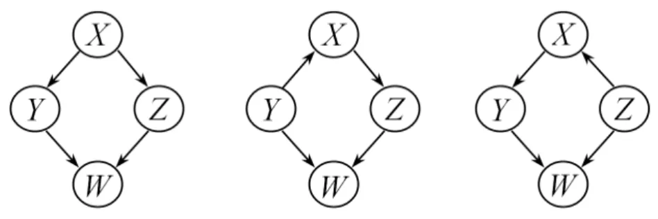
Figure 2.2: Three Markov equivalent DAGs. There are no other DAGs Markov equivalent to them.

2.2.2

Markov equivalence

Many DAGs are equivalent in the sense that they have the same d-separations. For example, each of the DAGs in figure 2.2 has the d-separations IG(Y, Z|X), IG(X, W|Y, Z) and these are the only d-separations each has. After stating a

formal definition of this equivalence, we give a theorem showing how it relates to probability distributions. Finally, we establish a criterion for recognizing this equivalence.

Definition 7 Let G1 =<U,E1 > and G2 =<U,E1 > be two DAGs containing

the same set of nodes U. Then G1 and G2 are called Markov equivalent if for

every three mutually disjoint subsets A,B,C ∈ U, A and B are d-separated by

C in G1 if and only if A and B are d-separated by C in G2. That is

IG1(A,B|C)⇔IG2(A,B|C)

Although the previous definition relates only to graph properties, its applica-tion is in probability, due to the following theorem:

Theorem 2 Two DAGs are Markov equivalent if and only if, based on the Markov condition, they entail the same conditional independences.

Proof. The proof follows immediately from theorem 1. ¤

Corollary 1 Let G1 =< U,E1 > and G2 =< U,E1 > be two DAGs containing

(26)

only if for every probability distribution P of U, (G1, P) satisfies the Markov

condition if and only if (G2, P) satisfies the Markov condition.

Proof. The proof follows immediately from theorems 1, 2. ¤

Next we present a theorem that shows how to identify Markov equivalence. Its proof requires the following three lemmas:

Lemma 4 Let G =< U,E > be a DAG, and X, Y ∈ U. Then X and Y are adjacent in G if and only if they are not d-separated by any set V⊆(U\X, Y).

Lemma 5 Suppose we have a DAG G =< U,E > and an uncoupled meeting

X−Z −Y. Then the following are equivalent:

• X−Z−Y is a head-to-head meeting.

• There exists a set not containing Z that d-separates X and Y.

• All sets containing Z do not d-separate X and Y.

Lemma 6 If G1 and G2 are Markov equivalent, then X and Y are adjacent in

G1 if and only if they are adjacent in G2. That is, Markov equivalent DAGs have

the same links (edges without regard for directions).

We now give the theorem that identifies Markov equivalence. This theorem was first stated in [Pearl et al. (1989)].

Theorem 3 Two DAGsG1 andG2 are Markov equivalent if and only if they have

the same links (edges without regard for direction) and the same set of uncoupled head-to-head meetings.

Theorem 3 gives us a simple way to represent a Markov equivalence class with a simple graph. That is, we can represent a Markov equivalence class with a graph that has the same links and the same uncoupled head-to-head meetings

(27)

as the DAGs in the class. Any assignment of directions to the undirected edges in this graph, that does no create a new uncoupled head-to-head meeting or a directed cycle, yields a member of the equivalence class. Often there are edges other than uncoupled head-to-head meetings which must be oriented the same in Markov equivalent DAGs. For example, if all uncoupled meeting X →Y −Z is not head-to-head, then all the DAGs in the equivalence class must have Y −Z

oriented as Y →Z. So we define aDAG patternfor a Markov equivalence class to be the graph that has the same links as the DAGs in the equivalence class and has oriented all and only the edges common to all of the DAGs in the equivalence class. The directed links in a DAG pattern are called compelled edges.

2.2.3

Embedded Faithfulness

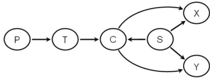
The distribution P(v, s, l, f) in figure 2.3 (b) does not admit a faithful DAG rep-resentation. However, it is the marginal of a distribution, namely P(v, s, c, l, f), which does. This is an example of embedded faithfulness, which is defined as follows:

Definition 8 Let P be a joint probability distribution of the variables inVwhere

V⊆U, and letG=<U,E> be a DAG. We say <G, P > satisfies the embed-ded faithfulness condition if the following two conditions holds:

• Based on the Markov condition, Gentails only conditional independences in

P for subsets including only elements of V.

• All conditional independences in P are entailed by G, based on the Markov condition.

When < G, P > satisfies the embedded faithfulness condition, we say P is

embedded faithfullyinG. Notice that faithfulness is a special case of embedded faithfulness in which U=V.

Theorem 4 Let P be a joint probability distribution of the variables in U with

V ⊆ U, and G =< U,E >. If < G, P > satisfies the faithfulness condition, and P0 _{is the marginal distribution of} _V_{, then} _< _G_{, P}0 _> _{satisfies the embedded}

faithfulness condition.

(28)

Figure 2.3: The marginal distribution of V, S, L and F cannot satisfy the faithfulness condition with any DAG.

Theorem 5 Let P be a joint probability distribution of the variables in V with

V ⊆ U, and G =< U,E >. Then < G, P > satisfies the embedded faithfulness condition if and only if all and only conditional independences in P are identified by d-separation in G restricted to elements of V.

2.2.4

Markov blankets and boundaries

A Bayesian network can have a large number of nodes, and the probability of a given node can be affected by instantiating a distant node. However, it turns out that the instantiation of a set of close nodes can shield a node from the effect of all other nodes. The following definition and theorem show this:

Definition 9 Let U be a set of random variables, P be their joint probability distribution, and X ∈ U. Then a Markov blanket MX of X is any set of

variables such that X is conditionally independent of all the other variables given

MX. That is,

IP(X,U\(MX ∪X)|MX)

Theorem 6 Suppose < G, P > satisfies the Markov condition. Then, for each variable X, the set of all parents of X, children of X and spouses of X is a Markov blanket of X.

(29)

2.3 Constraint-based structure learning

Definition 10 Let U be a set of random variables, P be their joint probability distribution, andX ∈U. Then a Markov boundary MBX of X is any Markov

blanket of X such that none of its proper subsets is a Markov blanket of X.

Theorem 7 Suppose < G, P > satisfies the faithfulness condition. Then, for each variable X, the set of all parents of X, children of X and spouses of X is the unique Markov boundary of X.

Theorem 7 holds for all probability distributions including ones that are not strictly positive. When a probability distribution is not strictly positive, there is not necessarily a unique Markov boundary. The final theorem presented in this section holds for strictly positive distributions.

Theorem 8 Suppose P is a strictly positive probability distribution of the vari-able in U. Then for eachX ∈U there is a unique Markov boundary of X.

Proof. The proof can be found in [Pearl (1988)]. ¤

2.3

Constraint-based structure learning

The problem of learning the most probable a posteriori BN from data is worst-case NP-hard [Chickering (2002); Chickering et al. (2004)] and the recent ex-plosion of high dimensional datasets poses a serious challenge to existing BN structure learning algorithms. Two types of BN structure learning methods have been proposed so far: score-and-search (a basic example is shown in algorithm 1) and constraint-based (a basic example is shown in algorithm 2) methods. While score-and-search methods are efficient for learning the full BN structure, the ability to scale up to hundreds of thousands of variables is a key advantage of constraint-based methods over score-and-search methods. The study presented in this thesis is focused on constraint-based approaches.

2.3.1

Soundness of constraint-based algorithms

Constraint-Based (CB for short) learning methods systematically check the data for conditional independence relationships. Typically, the algorithms run a χ2

(30)

Algorithm 1 DAG Pattern search: a basic score-and-search algorithm

Require: D: dataset; U: set of random variables.

Ensure: A DAG pattern (gp) that approximates maximizingscore(D, gp). 1: E← ∅

2: gp←(U,E) 3: repeat

4: if [any DAG pattern in the neighborhood of our current DAG pattern increases

score(D, gp)]then

5: modifyE according to the one that increases score(D, gp) the most 6: end if

7: until [score(D, gp) is not increased anymore]

independence test when the dataset is discrete and a Fisher’s Z-test when it is continuous in order to decide on dependence or independence, that is, upon the rejection or acceptance of the null hypothesis of conditional independence. A structure learning algorithm from data is said to be correct (or sound) if it returns the correct DAG pattern (or a DAG in the correct equivalence class) under the assumptions that the independence tests are reliable and that the learning dataset is a sample from a distribution P faithful to a DAG G, The (ideal) assumption that the independence tests are reliable means that they decide (in)dependence if and only if the (in)dependence holds in P. Based on what was just stated we next prove the soundness of algorithm 2.

Lemma 7 If the set of all conditional independences in Uadmit a faithful DAG representation, the algorithm 2 creates a link betweenX andY if and only if there is a link between X and Y in the DAG pattern gp containing the d-separations in this set.

Proof. The algorithm 2 produces a link if and only if X and Y are not d-separated by any subset of U, which, owing to Lemma 4, is the case if and only if X and Y are adjacent in gp. ¤

Lemma 8 If the set of all conditional independences in Uadmit a faithful DAG representation, then any directed edge created by the algorithm 2 is a directed edge in the DAG pattern containing the d-separations in this set.

(31)

Algorithm 2 DAG Pattern search: a basic constraint-based algorithm

Require: D: dataset; U: set of random variables.

Ensure: DAG pattern (gp) such thatIG(X, Y|Z)⇒IP(X, Y|Z). Step 1:

1: for all[pair of nodes X, Y ∈U]do

2: search for a subsetS_XY ⊆U such that I(X, Y|S_XY); 3: if [no such set can be found]then

4: create the link X−Y ingp; 5: end if

6: end for

Step 2:

7: for all[uncoupled meeting X−Z−Y]do 8: if [Z 6∈S_XY]then

9: orient X−Z−Y asX→Z ←Y; 10: end if

11: end for

Step 3:

12: for all[uncoupled meeting X→Z−Y]do 13: orient Z−Y asZ→Y;

14: end for

Step 4:

15: for all[link X−Y such that there is a path fromX toY]do 16: orient X−Y asX→Y;

17: end for

Step 5:

18: for all[uncoupled meetingX−Z−Y such thatX →W,Y →W andZ−W]do 19: orient Z−W asZ →W;

(32)

Proof. We consider the directed edges created in each step in turns:

Step 2: The fact that such edges must be directed follows from Lemma 5.

Step 3: If the uncoupled meetingX →Z−Y were X →Z ←Y, Z would not be in any set that d-separates X and Y due to Lemma 5, which means we would have created the orientation X → Z ← Y in Step 2. Therefore, X → Z −Y

must be X →Z →Y.

Step 4: If X−Y were X ←Y, we would have a directed cycle. Therefore, it must be X →Y.

Step 5: IfZ−W were Z ←W, then X−Z−Y would have to be X →Z ←Y

because otherwise we would have a directed cycle. But if this were the case, we would have created the orientation X → Z ← Y in Step 2. So Z −W must be

Z →W. ¤

Lemma 9 If the set of all conditional independences in U admit a faithful DAG representation, all the directed edges, in the DAG pattern containing the d-separations in this set, are directed by the algorithm 2.

Proof. The proof can be found in [Meek (1995)]. ¤

Theorem 9 If the set of all conditional independences in U admit a faithful DAG representation, the algorithm 2 creates the DAG pattern containing the d-separations in this set.

Proof. The proof follows from Lemmas 7, 8 and 9. ¤

2.3.2

G

likelihood-ratio conditional independence test

Statistical tests are needed in order to verify the conditional independence

I(X, Y|Z) from data. One of the most used statistical tests of conditional inde-pendence between two categorical variables is the G likelihood-ratio conditional independence test. In this thesis it is used to determine IP(X, Y|Z) from data

(33)

2.3 Constraint-based structure learning G= 2 m X i=1 p X j=1 q X k=1 n(i, j, k) ln n(i, j, k)n(·,·, k) n(i,·, k)n(·, j, k). (2.2)

where ln denotes the natural logarithm, n(i, j, k) is the number of times si-multaneously X = xi, Y = yj and Z =zk in the sample, that is, the value of the cell (i, j, k) in the contingency table. The sum is again taken over all non-empty cells. Given the null hypothesis of independence, the distribution of G is approximately that of chi-squared, with the same number of degrees of freedom as in the corresponding chi-squared test. The G-test returns a p-value, denoted as p, which is the probability of the error of assuming that the two variables are dependent when in fact they are not. We conclude independence if and only if p

is greater than a certain confidence threshold α.

A practical consideration regarding the reliability of a conditional indepen-dence test is the size of the conditioning set as measured by the number of vari-ables in the set, which in turn determines the number of values that the varivari-ables in the set may jointly take. Large conditioning sets produce sparse contingency tables and unreliable tests. This is why it is difficult to learn the neighborhood of a node having a large degree with CB methods. The number of possible configura-tions of the variables grows exponentially with the size of the conditioning set. In the experiments done in this thesis, the test is deemed unreliable if the number of instances is less than ten times the number of degrees of freedom as imple-mented inBNT Structure Learning Package for Matlab (http://banquiseasi.insa-rouen.fr/projects/bnt-slp/). Notice that there is no universal criterion: [Pe˜na

et al. (2007); Tsamardinos et al. (2006)] consider a test to be reliable when the number of instances is at least five times the number of degrees of freedom in the test, and when less than 20% of the contingency tables has less than 5 counts in [Bromberg et al. (2006)]. The exact criterion has little impact of the qualitative results though.

2.3.3

Fisher’s

Z

test

In the case of Gaussian Bayesian networks conditional independence can be tested by verifying if the partial correlation coefficient is zero. Suppose we are testing

(34)

whether the partial correlation coefficient ρ of Xi and Xj given S is zero. The

so-called Fisher’s Z is given by

Z = 1 2 p M − |S| −3 µ ln1 +R 1−R ¶ , (2.3)

whereM is the size of the sample, and R is a random variable whose value is the sample partial correlation coefficient of Xi and Xj given S. If we let

ζ = 1 2 p M − |S| −3 µ ln1 +ρ 1−ρ ¶ , (2.4)

then asymptotically Z−ζ has the standard normal distribution.

Suppose we wish to test the hypothesis that the partial correlation coefficient of Xi and Xj given S is ρ0 against the alternative hypothesis that is not. We

compute the value r of R, then the value z of Z, and let

ζ0 ₌ 1 2 p M− |S| −3 µ ln1 +ρ0 1−ρ0 ¶ . (2.5)

To test that the partial correlation coefficient is zero, we let ρ0 _{= 0 in}

expres-sion 2.5, which means that ζ0 _{= 0. For example, suppose we are testing whether} IP(X1, X2|X3), and the sample partial correlation coefficient of X1 and X2 given

X3 is 0.097 in a sample of size 20. Then

z = 1 2 √ 20−1−3¡ln1+0.097 1−0.097 ¢ = 0.389 and |z−ζ0_|₌_|0_.₃₈₉₋_0|_{= 0}_.₃₈₉

From a table for the standard normal distribution, if U has the standard normal distribution, then

P(|U|>0.389)≈0.7,

which means that we can reject the conditional independence for all and only significant levels greater than 0.7. For example, we could not reject it at a signif-icance level of 0.05.

(35)

2.4 Existence of a perfect map

2.4

Existence of a perfect map

The contents of this section is a synthesis of the study developed in [de Waal (2009)]. Definition 6 states when a probability distribution P and a DAG G

are faithful to each other. That is, when G is a perfect map (P-map) of P. The soundness of constraint-based algorithms is based on the assumption that there exists a DAG G such that G is a P-map of the probability distribution P. For every graphical independence model that is represented by d-separation in a directed acyclic graph, there exists an isomorphic probabilistic independence model, i.e. it has exactly the same independence statements. The reverse does not hold, as there exist probability distributions for which there are no perfect maps.

Probabilistic models in artificial intelligence are typically built on the semi-graphoids axioms of independence. These axioms are exploited explicitly in graphical models, where independence is captured by topological properties, such as separation of vertices in an undirected graph or d-separation in a directed graph. A graphical representation with directed graphs for use in a decision support system has the advantage that it allows an intuitive interpretation by domain experts in terms of influences between the variables. Ideally the prob-abilistic model should be isomorphic with the graphical model, and vice versa. That is, the graphical and the probabilistic model should be faithful to each other. A set of necessary conditions for directed graph isomorphism is given in [Pearl (1988)]. However, there is no known set of sufficient conditions.

In [Pearl (1988)] an example was provided of an independence model not iso-morphic with a directed graphical model, that can be made isoiso-morphic by the introduction of an auxiliary variable. The isomorphism is then established in [Pearl (1988)] by conditioning on the auxiliary variable. A different approach is presented in [de Waal (2009)], where the model is extended with auxiliary vari-ables to a directed graph isomorph and then only the marginal over the original variables of this extended model is taken. The model with auxiliary variables can then be considered as a latent perfect map. [de Waal (2009)] shown that it is possible to establish isomorphism in this manner, but that an infinite number of auxiliary variables may be needed to accomplish this. Both approaches are not

(36)

discussed in this thesis (see [de Waal (2009); Pearl (1988)] for more information). However, we judge important some brief review about independence models in order to better understand the applicability and limitations of the approaches presented in this thesis. Next we provide some preliminaries on probabilistic independence models as defined by conditional independence for probability dis-tributions, graphical independence models as defined by d-separation in directed acyclic graphs, and algebraic independence models that capture the properties that probabilistic and graphical models have in common.

2.4.1

Conditional independence models

Let us consider a finite set of distinct symbols V = {V1, ..., VN}, called the

at-tributes or variables names. With each variable Vi we associate a finite domain

set Vi, which is the set of possible values the variable can take. We define the

domain of V as V=V1×...×VN, the Cartesian product of the domains of the

individual variables.

Aprobability measureoverVis defined by the domainsVi, i= 1, ..., N (sample

space), and a probability mapping P : V → [0,1] (probability function) that satisfies the three basic axioms of probability theory described by theorem 10. The conditions in this theorem were labeled theaxioms of probability theory by A.N. Kolmogorov in 1933.

Theorem 10 Let Ω be a sample space and P be a probability function. Then the pair (Ω, P) is called a probability space and the three following con-ditions are observed:

• P(Ω) = 1.

• 0≤P(E)≤1 for every E⊆Ω.

• For E and F⊆Ω such that E∩F=∅, P(E∪F) = P(E) +P(F).

Proof. The proof can be found in [Kolmogorov (1950)]. ¤

For any subsetX={Vi1, ..., Vik} ⊂V, for some K ≥1, we define the domain

(37)

marginal mapping overX, denoted byPX, as the probability measure PX over

X, defined by

PX(x) =P{P(x, y)|y∈(×Vi,∀i|Vi 6∈X)}

for x∈X. By definition PV ≡P, P∅ _≡ _{1, and (}_PX₎Y _{= (}_PY₎X ₌_PX∩Y_,

for X,Y∈V.

We denote the set of ordered triplets (X,Y|Z) for disjoint subsetsX,YandZ ofVasI(V). For any ternary relationIonVwe shall use the notationI(X,Y|Z) to indicate (X,Y|Z) ∈ I. For simplicity of notation we will often write XY to denote the union X∪Y, for X,Y ⊂V. To avoid complicated notation we also allow Xy to denote X∪y, for X⊂V and y∈V.

Definition 11 (Conditional independence). Let X, Y and Z be disjoint subsets of V, with domains X, Y and Z, respectively. The sets X and Y are defined to be conditionally independent under P given Z, if for every x ∈ X,

y ∈Y and z ∈Z, we have

PXYZ(x, y, z).PZ(z) =PXZ(x, z).PYZ(y, z)

Definition 12 Let V be a set of variables and P a probability measure over

V. The probabilistic independence model IP of P is defined as the ternary

relation IP on Vfor which IP(X,Y|Z) if and only if X and Y are conditionally

independent under P given Z.

If no ambiguity can arise we may omit the reference to the probability measure and just refer to the probabilistic independence model.

2.4.2

Graphical independence models

The standard concepts of d-separation in directed acyclic graphs have already been thoroughly discussed in section 2.2. Here we just give some additional Comments. Definition 1 states when a chain ρis blocked in a DAGG by a setZ. We refer to the first two conditions in Definition 1 as blocking by presence, and the last conditions as blocking by absence. We sometimes refer to head-to-head nodeZ in the last condition as aconverging orcolliding nodeon the

(38)

chain. While the concept of blocking is defined for a single chain, the d-separation criterion applies to the set of all chains in G, as it is stated by definition 2. Definition 13 Let G= (V,E) be a DAG. The graphical independence model IG

defined by G is a ternary relation on V such that IG(X,Y|Z) if and only if Z

d-separates Xand Yin G.

2.4.3

Algebraic independence models

Both a probabilistic independence model on a set of variables V and a graphical independence model on a DAGG= (V,E) define a ternary relation onV. In fact we can capture this in an algebraic construction of an independence model. Definition 14 An algebraic independence model on a set V is a ternary relation on V.

Probabilistic and graphical independence models satisfy a set of axioms of independence. We use these axioms to define a special class within the set of algebraic independence models.

Definition 15 A ternary relation I on V is a semi-graphoid independence model, or semi-graphoid for short, if it satisfies the following four axioms:

• symmetry: I(X,Y|Z)⇒I(Y,X|Z),

• decomposition: I(X,YW|Z)⇒I(X,Y|Z)∧I(X,W|Z),

• weak union: I(X,YW|Z)⇒I(X,Y|ZW),

• contraction: I(X,Y|Z)∧I(X,W|ZY)⇒I(X,YW|Z). For all disjoint sets of variables W,X,Y,Z∈V.

The axioms convey the idea that learning irrelevant information does not alter the relevance relationships among the other variables discerned. They were first introduced in [Dawid (1979)] for probabilistic conditional independence. The properties were later recognized in artificial intelligence as properties of separation

(39)

in graphs [Pearl (1988); Pearl & Paz (1987)], and are since known as the semi-graphoid axioms.

In the formulation that we have used so far we can allowXandYto be empty, which leads to the so called trivial independence axiom: I(X,∅|Z). This axiom trivially holds for both probabilistic independence and graphical independence.

An axiomatic representation allows us to derive qualitative statements about conditional independence that may not be immediate from a numerical repre-sentation of probabilities. It also enables a parsimonious specification of an in-dependence model, since it is sufficient to enumerate the so-called dominating independence statements, from which all other statements can be derived by ap-plication of the axioms [Studen´y (1998)].

2.4.4

Graph-Isomorph

Probabilistic independence models and graphical independence models both sat-isfy the semi-graphoid axioms, so it is interesting to investigate whether they have equal modelling power. Can any probabilistic independence model be rep-resented by a graphical model, and vice versa? For this we introduce the notions of DAG-isomorph.

Definition 16 An independence modelIonV, is said to be aDAG-isomorph, if there exists a graph G= (V,E) that is a perfect map for I.

Since a graphical independence model satisfies the semi-graphoid axioms, a DAG-isomorph has to be a semi-graphoid itself. Being a semi-graphoid is not a sufficient condition for DAG-isomorphism, however. It seems that there does not exist a sufficient set of conditions, although Pearl presents a set of necessary conditions in [Pearl (1988)].

Some results from literature describe the modelling powers of the types of independence models presented in the previous sections. Geiger and Pearl show that for every DAG graphical model there exists a probability model for which that particular DAG is a perfect map [Geiger & Pearl (1990)]. The reverse does not hold, there exist probability models for which there is no DAG perfect map [Pearl (1988)].

(40)

Studen´y shows in [Studen´y (1989)] that the semi-graphoid axioms are not complete for probabilistic independence models. He derives a new axiom for probabilistic independence models