Job Scheduling for Multi-User MapReduce Clusters
Matei Zaharia
Dhruba Borthakur
Joydeep Sen Sarma
Khaled Elmeleegy
Scott Shenker
Ion Stoica
Electrical Engineering and Computer Sciences
University of California at Berkeley
Technical Report No. UCB/EECS-2009-55
http://www.eecs.berkeley.edu/Pubs/TechRpts/2009/EECS-2009-55.html
April 30, 2009
Copyright 2009, by the author(s).
All rights reserved.
Permission to make digital or hard copies of all or part of this work for
personal or classroom use is granted without fee provided that copies are
not made or distributed for profit or commercial advantage and that copies
bear this notice and the full citation on the first page. To copy otherwise, to
republish, to post on servers or to redistribute to lists, requires prior specific
permission.
Acknowledgement
We would like to thank the Hadoop teams at Yahoo! and Facebook for the
discussions based on practical experience that guided this work. We are
also grateful to Joe Hellerstein and Hans Zeller for their pointers to related
work in database systems. This research was supported by California
MICRO, California Discovery, the Natural Sciences and Engineering
Research Council of Canada, as well as the following Berkeley Reliable
Adaptive Distributed systems lab sponsors: Sun Microsystems, Google,
Microsoft, HP, Cisco, Facebook and Amazon.
Job Scheduling for Multi-User MapReduce Clusters
Matei Zaharia
†Dhruba Borthakur
‡Joydeep Sen Sarma
‡Khaled Elmeleegy
∗Scott Shenker
†Ion Stoica
† †University of California, Berkeley
‡Facebook Inc
∗Yahoo! Research
[email protected] {dhruba,jssarma}@facebook.com [email protected] {istoica,shenker}@cs.berkeley.edu
Abstract
Sharing a MapReduce cluster between users is attractive because it enables statistical multiplexing (lowering costs) and allows users to share a common large data set. How-ever, we find that traditional scheduling algorithms can perform very poorly in MapReduce due to two aspects of the MapReduce setting: the need for data locality (run-ning computation where the data is) and the dependence between map and reduce tasks. We illustrate these prob-lems through our experience designing a fair scheduler for MapReduce at Facebook, which runs a 600-node multi-user data warehouse on Hadoop. We developed two simple techniques, delay scheduling and copy-compute splitting, which improve throughput and response times by factors of 2 to 10. Although we focus on multi-user workloads, our techniques can also raise throughput in a single-user, FIFO workload by a factor of 2.
1
Introduction
MapReduce and its open-source implementation Hadoop [2] were originally optimized for large batch jobs such as web index construction. However, another use case has recently emerged: sharing a MapReduce cluster between multiple users, which run a mix of long batch jobs and short interactive queries over a common data set. Sharing enablesstatistical multiplexing, leading to lower costs over building private clusters for each group. Sharing a cluster also leads to data consolidation (colocation of disparate data sets). This avoids costly replication of data across private clusters, and lets an organization run unanticipated queries across disjoint datasets efficiently.
Our work was originally motivated by the MapReduce workload at Facebook, a major web destination that runs a data warehouse on Hadoop. Event logs from Facebook’s website are imported into a Hadoop cluster every hour, where they are used for a variety of applications, including analyzing usage patterns to improve site design, detecting spam, data mining and ad optimization. The warehouse runs on 600 machines and stores 500 TB of compressed data, which is growing at a rate 2 TB per day. In addition to “production” jobs that must run periodically, there are many experimental jobs, ranging from multi-hour machine learning computations to 1-2 minute ad-hoc queries sub-mitted through a SQL interface to Hadoop called Hive [3].
The system runs 3200 MapReduce jobs per day and has been used by over 50 Facebook engineers.
As Facebook began building its data warehouse, it found the data consolidation provided by a shared cluster highly beneficial. For example, an engineer working on spam de-tection could look for patterns in arbitrary data sources, like friend lists and ad clicks, to identify spammers. How-ever, when enough groups began using Hadoop, job re-sponse times started to suffer due to Hadoop’s FIFO sched-uler. This was unacceptable for production jobs and made interactive queries impossible, greatly reducing the utility of the system. Some groups within Facebook considered building private clusters for their workloads, but this was too expensive to be justified for many applications.
To address this problem, we have designed and imple-mented a fair scheduler for Hadoop. Our scheduler gives each user the illusion of owning a private Hadoop cluster, letting users start jobs within seconds and run interactive queries, while utilizing an underlying shared cluster effi-ciently. During the development process, we have uncov-ered several scheduling challenges in the MapReduce set-ting that we address in this paper. We found that exisset-ting scheduling algorithms can behave very poorly in MapRe-duce, degrading throughput and response time by factors of 2-10, due to two aspects of the setting: data locality (the need to run computations near the data) and interdepen-dence between map and reduce tasks. We developed two simple, robust algorithms to overcome these problems: de-lay scheduling and copy-compute splitting. Our techniques provide 2-10x gains in throughput and response time in a multi-user workload, but can also increase throughput in asingle-user, FIFOworkload by a factor of 2. While we present our results in the MapReduce setting, they gener-alize to any data flow based cluster computing system, like Dryad [20]. The locality and interdependence issues we address are inherent in large-scale data-parallel computing. There are two aspects that differentiate scheduling in MapReduce from traditional cluster scheduling [12]. The first aspect is the need fordata locality, i.e., placing tasks on nodes that contain their input data. Locality is crucial for performance because the network bisection bandwidth in a large cluster is much lower than the aggregate band-width of the disks in the machines [16]. Traditional clus-ter schedulers that give each user a fixed set of machines,
like Torque [12], significantly degrade performance, be-cause files in Hadoop are distributed across all nodes as in GFS [19]. Grid schedulers like Condor [22] support lo-cality constraints, but only at the level of geographic sites, not of machines, because they run CPU-intensive appli-cations rather than data-intensive workloads like MapRe-duce. Even with a granular fair scheduler, we found that lo-cality suffered in two situations: concurrent jobs and small jobs. We address this problem through a technique called delay scheduling that can double throughput.
The second aspect of MapReduce that causes problems is the dependence between map and reduce tasks: Re-duce tasks cannot finish until all the map tasks in their job are done. This interdependence, not present in tradi-tional cluster scheduling models, can lead to underutiliza-tion and starvaunderutiliza-tion: a long-running job that acquires reduce slots on many machines will not release them until its map phase finishes, starving other jobs while underutilizing the reserved slots. We propose a simple technique called copy-compute splittingto address this problem, leading in 2-10x gains in throughput and response time. The reduce/map de-pendence also creates other dynamics not present in other settings: for example, even with well-behaved jobs, fair sharing in MapReduce can take longer to finish a batch of jobs than FIFO; this is not true environments, such as packet scheduling, where fair sharing is work conserving. Yet another issue is that intermediate results produced by the map phase cannot be deleted until the job ends, con-suming disk space. We explore these issues in Section 7.
Although we motivate our work with the Facebook case study, the problems we address are by no means con-strained to a data warehousing workload. Our contacts at another major web company using Hadoop confirm that the biggest complaint users have about the research clus-ters there is long queueing delays. Our work is also rel-evant to the several academic Hadoop clusters that have been announced. One such cluster is already using our fair scheduler on 2000 nodes. In general, effective scheduling is more important in data-intensive cluster computing than in other settings because the resource being shared (a clus-ter) is very expensive and because data is hard to move (so data consolidation provides significant value).
The rest of this paper is organized as follows. Section 2 provides background on Hadoop and problems with previ-ous scheduling solutions for Hadoop, including a Torque-based scheduler. Section 3 presents our fair scheduler. Section 4 describes data locality problems and our delay scheduling technique to address them. Section 5 describes problems caused by reduce/map interdependence and our copy-compute splitting technique to mitigate them. We evaluate our algorithms in Section 6. Section 7 discusses scheduling tradeoffs in MapReduce and general lessons for job scheduling in cluster programming systems. We survey related work in Section 8 and conclude in Section 9.
Figure 1: Data flow in MapReduce. Figure from [4].
2
Background
Hadoop’s implementation of MapReduce resembles that of Google [16]. Hadoop runs on top of a distributed file sys-tem, HDFS, which stores three replicas of each block like GFS [19]. Users submitjobsconsisting of a map function and a reduce function. Hadoop breaks each job into mul-tiple tasks. First, map tasks process each block of input (typically 64 MB) and produceintermediate results, which are key-value pairs. These are saved to disk. Next, re-duce tasksfetch the list of intermediate results associated with each key and run it through the user’s reduce func-tion, which produces output. Each reducer is responsible for a different portion of the key space. Figure 1 illustrates a MapReduce computation.
Job scheduling in Hadoop is performed by a master node, which distributes work to a number ofslaves. Tasks are assigned in response toheartbeats(status messages) re-ceived from the slaves every few seconds. Each slave has a fixed number ofmap slotsandreduce slotsfor tasks. Typi-cally, Hadoop tasks are single-threaded, so there is one slot per core. Although the slot model can sometimes under-utilize resources (e.g., when there are no reduces to run), it makes managing memory and CPU on the slaves easy. For example, reduces tend to use more memory than maps, so it is useful to limit their number. Hadoop is moving towards more dynamic load management for slaves, such as taking into account tasks’ memory requirements [5]. In this pa-per, we focus on scheduling problems above the slave level. The issues we identify and the techniques we develop are independent of slave load management mechanism.
2.1 Previous Scheduling Solutions for Hadoop
Hadoop’s built-in scheduler runs jobs in FIFO order, with five priority levels. When a task slot becomes free, the scheduler scans through jobs in order of priority and submit time to find one with a task of the required type1. For maps, the scheduler uses a locality optimization as in Google’s 1With memory-aware load management [5], there is also a check that
MapReduce [16]: after selecting a job, the scheduler picks the map task in the job with data closest to the slave (on the same node if possible, otherwise on the same rack, or fi-nally on a remote rack). Fifi-nally, Hadoop usesbackup tasks to mitigate slow nodes as in [16], but backup scheduling is orthogonal to the problems we study in this paper.
The disadvantage of FIFO scheduling is poor response times for short jobs in the presence of large jobs. The first solution to this problem in Hadoop was Hadoop On Demand (HOD) [6], which provisions private MapReduce clusters over a large physical cluster using Torque [12]. HOD lets users share a common filesystem (running on all nodes) while owning private MapReduce clusters on their allocated nodes. However, HOD had two problems:
• Poor Locality:Each private cluster runs on a fixed set of nodes, but HDFS files are divided across all nodes. As a result, some maps must read data over the net-work, degrading throughput and response time. One trick to address this is to make each HOD cluster have at least one node per rack, letting data be read over rack switches [10], but this is not enough if rack bandwidth is less than the bandwidth of the disks on each slave. • Poor Utilization: Because each private cluster has a
static size, some nodes in the physical cluster may be idle. This is suboptimal because Hadoop jobs are “elastic,” unlike traditional HPC jobs, in that they can change how many nodes they are running on over time. Idle nodes could thus go towards speeding up jobs.
3
The FAIR Scheduler Design
To address the problems with HOD, we developed a fair scheduler, simply called FAIR, for Hadoop at slot-level granularity. Our scheduler has two main goals:
• Isolation: Give each user (job) the illusion of owning (running) a private cluster.
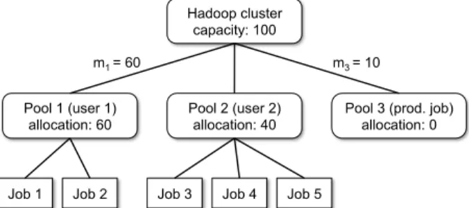
• Statistical Multiplexing: Redistribute capacity un-used by some users (jobs) to other users (jobs). FAIR uses a two-level hierarchy. At the top level, FAIR allocates task slots across “pools”, and at the second level, each pool allocates its slots among multiple jobs in the pool. Figure 2 shows an example hierarchy. While in our design and implementation we used a two level hier-archy, FAIR can be easily generalized to more levels.
FAIR uses a version of max-min fairness [8] with min-imum guarantees to allocate slots across pools. Each pool i is given a minimum share (number of slots) mi, which
can be zero. The scheduler ensures that each pool will re-ceive its minimum share as long as it has enough demand, and the sum over the minimum shares of all pools does not exceed the system capacity. When a pool is not using its full minimum share, other pools are allowed to use its slots. In practice, we create one pool per user and special pools for production jobs. This gives users (pools) perfor-mance at least as good as they would have had in a private
Hadoop cluster capacity: 100 Pool 2 (user 2) allocation: 40 Pool 1 (user 1) allocation: 60
Pool 3 (prod. job) allocation: 0
Job 1 Job 2 Job 3 Job 4 Job 5
m1 = 60 m3 = 10
Figure 2: Example of allocations in our scheduler. Pools 1 and 3 have minimum shares of 60, and 10 slots, respectively. Because Pool 3 is not using its share, its slots are given to Pool 2.
Hadoop cluster equal in size to their minimum share, but often higher due to statistical multiplexing.
FAIR uses the same scheduling algorithm to allocate slots among jobs in the same pool, although other schedul-ing disciplines, such as FIFO and multi-level queueschedul-ing, could be used.
3.1 Slot Allocation Algorithm
We formally describe FAIR in Appendix 10. Here, we give one example to give the reader a notion of how it works.
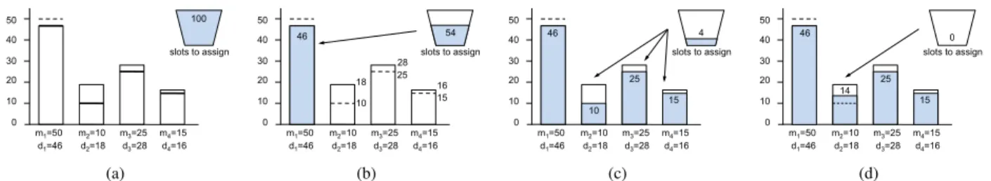
Figure 3 illustrates an example where we allocate 100 slots among four pools with the following minimum shares mi and demands di: (m1=50,d1=46), (m1=10,d1= 18),(m1=25,d1=28), (m4=15,d4=16). We visual-ize each pool as a bucket, the svisual-ize of which represents the pool’s demand. Each bucket also has a mark represent-ing its minimum share. If pool’s minimum share is larger than its demand, the bucket has no mark. The allocation reduces to pouring water into the buckets, where the total volume of water represents the number of slots in the sys-tem. FAIR operates in three phases. In the first phase, it fills each unmarked bucket, i.e., it satisfies the demand of each bucket whose minimum share is larger than its demand. In the second phase, it fills all remaining buckets up to their marks. With this step, the isolation property is enforced as each bucket has received either its minimum share, or its demand has been satisfied. In the third phase, FAIR im-plements statistical multiplexing by pouring the remaining water evenly into unfilled buckets, starting with the bucket with the least water and continuing until all buckets are full or the water runs out. The final shares of the pools are 46 for pool 1, 14 for pool 2, 25 for pool 3 and 15 for pool 4, which is as close as possible to fair while meeting mini-mum guarantees.
3.2 Slot Reassignment
As described above, at all times, FAIR aims to allocate the entire capacity of the clusters among pools that have jobs. A key question is how to reassign the slots when demand changes. Consider a system with 100 slots and two pools which use 50 slots each. When a third pool becomes ac-tive, assume FAIR needs to reallocate the slots such that each pool gets roughly 33 slots. There are three ways to
m1=50 d1=46 m2=10 d2=18 m3=25 d3=28 m4=15 d4=16 10 20 30 40 50 0 100 slots to assign (a) m1=50 d1=46 m2=10 d2=18 m3=25 d3=28 m4=15 d4=16 10 20 30 40 50 0 slots to assign 46 54 10 25 16 18 28 15 (b) m1=50 d1=46 m2=10 d2=18 m3=25 d3=28 m4=15 d4=16 10 20 30 40 50 0 4 slots to assign 46 10 25 15 (c) m1=50 d1=46 m2=10 d2=18 m3=25 d3=28 m4=15 d4=16 10 20 30 40 50 0 0 slots to assign 46 14 25 15 (d)
Figure 3: Slot allocation example. Figure (a) shows pool demands (as boxes) and minimum shares (as dashed lines). The algorithm proceeds in three phases: fill buckets whose minimum share is more than their demand (b), fill remaining buckets up to their minimum share (c), and distribute remaining slots starting at the emptiest bucket (d).
free slots for the new job: (1) kill tasks of other pools’ jobs, (2) wait for tasks to finish, or (3) preempt tasks (and resume them later). Killing a task allows FAIR to imme-diately re-assign the slot, but it wastes the work performed by the task. In contrast, waiting for the task to finish delays slot reassignment. Task preemption enables immediate re-assignment and avoids wasting work, but it is complex to implement, as Hadoop tasks run arbitrary user code. FAIR uses a combination of approaches (1) and (2).
When a new job starts, FAIR starts allocating slots to it as other jobs’ tasks finish. Since MapReduce tasks are typically short (15-30s for maps and a few minutes for reduces), a job will achieve its fair share (as computed by FAIR) quite fast. For example, if tasks are one minute long, then every minute, we can reassign every slot in the cluster. Furthermore, if the new job only needs 10% of the slots, it gets them in 6 seconds on average. This makes launch delays in our shared cluster comparable to delays in private clusters.
However, there can be cases in which jobs do have long tasks, either due to bugs or due to non-parallelizable computations. To ensure that each job gets its share in those cases, FAIR uses two timeouts, one for guaranteeing the minimum share (Tmin), and another one for
guarantee-ing the fair share (Tf air), whereTmin<Tf air. If a newly
started job does not get its minimum share beforeTmin
ex-pires, FAIR kills other pools’ tasks and re-allocates them to the job. Then, if the job has not achieved its fair share by Tf air, FAIR kills more tasks. When selecting tasks to kill,
we pick the most recently launched tasks in over-scheduled jobs to minimize wasted computation, and we never bring a job below its fair share. Hadoop jobs tolerate losing tasks, so a killed task is treated as if it never started. While killing tasks lowers throughput, it lets us meet our goal of giving each user the illusion of a private cluster. User isolation outweighs the loss in throughput.
3.3 Obstacles to Fair Sharing
After deploying an initial version of FAIR, we identified two aspects of MapReduce which have a negative impact on the performance (throughput, in particular) of FAIR. Since these aspects are not present in the tradiotional HPC scheduling we discuss them in detail:
• Data Locality: MapReduce achieves its efficiency by running tasks on the nodes that contain their input data, but we found that a strict implementation of fair shar-ing can break locality. This problem also happens with strict implementations of other scheduling disciplines, including FIFO in Hadoop’s default scheduler.
• Reduce/Map Interdependence:Because reduce tasks
must wait for their job’s maps to finish before they can complete, they may occupy a slot for a long time, starv-ing other jobs. This also leads to underutilization of the slot if the waiting reduces have little data to copy. The next two sections explain and address these problems.
4
Data Locality
The first aspect of MapReduce that poses scheduling chal-lenges is the need to place computation near the data. This increases throughput because network bisection bandwidth is much smaller in a large cluster than the total bandwidth of the cluster’s disks. Running on a node that contains the data (node localityis most efficient, but when this is not possible, running on the same rack (rack locality) provides better performance than being off-rack. Rack interconnects are usually 1 Gbps, whereas bandwidth per node at an ag-gregation switch can be 10x lower. Rack bandwidth may still be less than the total bandwidth of the disks on each node, however. For example, Facebook’s nodes have 4 disks, with a bandwidth of 50-60 MB/s each or 2 Gbps in total, while its rack links are 1 Gbps.
We describe two locality problems observed at Face-book, followed by a technique called delay scheduling to address them. We analyze delay scheduling in Section 4.3 and explain a refinement, IO-rate biasing, for handling hotspots.
4.1 Locality Problems
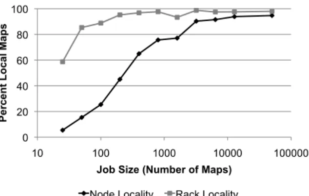
The first locality problem we saw was in small jobs. Fig-ure 4 shows locality for jobs of different sizes (number of maps) running in production at Facebook over a month. Each point represents a bin of sizes. The first point is for jobs with 1 to 25 maps, which only achieve 5% node local-ity and 59% rack locallocal-ity. In fact,58%of jobs at Facebook fall into this bin, because small jobs are common for ad-hoc queries and hourly reports in a data warehouse.
head-of-0 20 40 60 80 100 10 100 1000 10000 100000
Percent Local Maps
Job Size (Number of Maps) Node Locality Rack Locality
Figure 4: Data locality vs. job size in production at Facebook.
0 10 20 30 40 50 60 70 80 90 100 0 2 4 6 8 10 12 14 16 18 20
Expected Node Locality (%)
Number of Concurrent Jobs
Figure 5: Expected effect of sticky slots in 100-node cluster.
line scheduling. At any time, there is a single job that must be scheduled next according to fair sharing: the job farthest below its fair share. Any slave that requests a task is given one from this job. However, if the head-of-line job is small, the probability that blocks of its input are available on the slave requesting a task is low. For example, a job with data on 10% of nodes achieves 10% locality. This problem is present in all current Hadoop schedulers, including the FIFO scheduler, because they all give tasks to the first job in some ordering (by submit time, fair share, etc).
A related problem,sticky slots, happens even with large jobs if fair sharing is used. Suppose, for example, that there are 10 jobs in a 100-node cluster with one slot per node, and each is running 10 tasks. Suppose Job 1 finishes a task on node X. Node X sends a heartbeat requesting a new task. At this point, Job 1 has 9 tasks running while all other jobs have 10. Therefore, Job 1 is assigned the slot on node X again. Consequently, in steady state,jobs never leave their original slots. This leads to poor locality as in HOD, because input files are distributed across the cluster. Locality can be low even with few jobs. Figure 5 shows expected locality in a 100-node cluster with 3-way block replication and one slot per node as a function of number of concurrent jobs. Even with 5 jobs, locality is below 50%.
Sticky slots do not occur in Hadoop due to a bug in how Hadoop counts running tasks. Hadoop tasks enter a “com-mit pending” state after finishing their work, where they request permission to rename their output to its final file-name. The job object in the master counts a task in this
state as running, whereas the slave object doesn’t. There-fore another job can be given the task’s slot. While this is bug (breaking fairness), it has limited impact on through-put and response time. Nonetheless, we explain sticky slots to warn other system designers of the problem. In Section 6, we show that sticky slots lower throughput by 2x in a modified version of Hadoop without this bug.
4.2 Our Solution: Delay Scheduling
The problems we presented stem from a lack ofchoicein the scheduler: following a strict queueing order forces a job with no local data to be scheduled. We address them through a simple technique called delay scheduling. When a node requests a task, if the head-of-line job cannot launch a local task, we skip this job and look at subsequent jobs. However, if a job has been skipped long enough, we let it launch non-local tasks, avoiding starvation. In our sched-uler, we use two wait times: jobs waitT1 seconds before being allowed to launch non-local tasks on the same rack andT2more seconds before being allowed to launch off-rack. We found that settingT1andT2as low as 15 seconds can bring locality from 2% to 80% even in a pathological workload with very small jobs and can double throughput. Formal pseudocode for delay scheduling is as follows: Algorithm 1Delay Scheduling
Maintain three variables for each job j, initialized asj.level=
0, j.wait=0, andj.skipped=f alse.
ifa heartbeat is received from nodenthen
for each jobjwithj.skipped=true, increasej.waitby the time since last heartbeat and setj.skipped=f alse
ifnhas a free map slotthen
sort jobs in by distance below min and fair share
for jin jobsdo
ifjhas a node-local tasktfornthen
set j.wait=0 andj.level=0 returntton
else if jhas rack-local tasktonnand (j.level≥1 or
j.wait≥T1)then
set j.wait=0 andj.level=1 returntton
else if j.level=2 or (j.level=1 and j.wait≥T2) or
(j.level=0 andj.wait≥T1+T2)then
set j.wait=0 andj.level=2 returntton
else
set j.skipped=true
end if end for end if end if
Each job begins at a locality level of 0, where it can only launch node-local tasks. If it waits at leastT1 seconds, it goes to locality level 1 and may launch rack-local tasks. If it waits a furtherT2seconds, it goes to level 2 and may launch off-rack tasks. It is straightforward to add more
lo-cality levels for clusters with more than a two-level net-work hierarchy. Finally, if a job ever launches a “more local” task than the level it is on, it goes back to a previous level. This ensures that a job that gets unlucky early in its life will not always keep launching non-local tasks.
Delay scheduling performs well even with values ofT1 andT2as small as 15 seconds. This happens because map tasks tend to be short (10-20s). Even if each map is 60s long, in 15 seconds, we have a chance to launch tasks on 25% of the slots in the cluster, assuming tasks finish uni-formly throughout time. Because nodes have multiple map slots (5 at Facebook) and each block has multiple replicas (usually 3), the chance of launching on a localnodeis high. For example, with 5 slots per node and 3 replicas, there are 15 slots in which a task can run. The probability of at least one of them freeing up in 15s is 1−(3/4)15=98.6%.
4.3 Analysis
We analyzed delay scheduling from two perspectives: min-imizing response times and maxmin-imizing throughput. Our goal was to determine how the algorithm behaves as a func-tion of the values of the delays,T1 andT2. Through this analysis, we also derived a refinement called IO-rate bias-ing for handlbias-ing hotspots more efficiently.
4.3.1 Response Time Perspective
We used a simple mathematical model to determine how waits should be set if the only goal is to provide the best response time for a given job. In this model, we assume that competing map tasks don’t affect each other’s band-width – perhaps because the bulk of the bandband-width in the cluster is used by reduce tasks, or because the job is small (which is 10-15s of response time matter). Instead, a non-local map just takesDseconds longer to run than a local map. Ddepends on the task; it might be 0 for CPU-bound jobs. We model the arrival of task requests at the master as a Poisson process where requests from nodes with local data arrive at a rate of one everytseconds. This is a good approximation if there are enough slots with local data re-gardless of the distribution of task lengths, by the Law of Rare Events. Suppose that we set the wait time for launch-ing tasks locally tow. We calculated the expected gain in a task’s response time from delay scheduling, as opposed to launching it on the first request received, to be:
E(gain) = (1−e−w/t)(D−t) (1) A first implication of this result is that delay scheduling is worthwhile ifD>t. Intuitively, waiting is worthwhile if the delay from running non-locally is less than the expected wait for a local slot. This happens because 1−e−w/t is
always positive, so the sign of the gain is determined by D−t. Waiting might not be worthwhile in two conditions: ifDis low (e.g. the job is not IO-bound) or iftis high (the job has few maps left or the cluster is running long tasks).
A second implication is that when D>t, the optimal wait time is infinity. This is because 1−e−w/t approaches
1 aswincreases. This result might seem counterintuitive, but it follows from the Poisson nature of our task request arrival model: if waiting used to be worthwhile because D>t and we have waited some time and not received a local task request, thenDis still greater thant so waiting is still worthwhile. In practice, infinite delays do not make sense, but we see that expected gain grows withwand lev-els out fast (for example, ifw=2tthen 1−e−w/t=0.86). Therefore, delays can be set to bound worst-case response time, rather than needing to be carefully tuned.
In conclusion, a scheduler optimizing only for response time should launch CPU-bound right away but use delay scheduling for IO-bound jobs, except maybe towards the end of the job when only a few tasks are left to run.
4.3.2 Throughput Perspective
From the point of view of throughput, if there are many jobs running and load across nodes is balanced, it is always worthwhile to skip jobs that cannot launch local tasks – a job further in the queue will have a task to launch. How-ever, there is a problem if there’s a “hotspot” node that many jobs want to run on: this node becomes a bottleneck, while other nodes are left idle. Setting the wait thresholds to any reasonably small value will prevent this, because the tasks waiting on the hotspot will be given to other nodes. If the tasks waiting on the hotspot have similar performance characteristics, there will be no impact on throughput.
A refinement can be made when the tasks waiting on the hotspot have different performance characteristics. In this case, it is best tolaunch CPU-intensive tasks non-locally, while running IO-bound tasks locally. We call this policy IO-rate biasing. IO-rate biasing helps because CPU-bound tasks read data at a lower rate than IO-bound tasks, and therefore, running them remotely places less load on the network than running IO-bound tasks remotely. For exam-ple, suppose that two types of tasks waiting on a hotspot node: IO-bound tasks from Job 1 that take 5s to process a 64 MB block, and CPU-bound tasks from Job 2 that take 25s to process a block. If the scheduler launches a task from Job 1 remotely, this task will try to read data over the network at 64MB/5s = 12.8 MB/s. If this bandwidth can’t be met, the task will run longer than 5s, decreasing over-all throughput (rate of task completion). Even if the 12.8 MB/s can be provided, this flow will compete with reduce traffic, decreasing throughput. On the other hand, if the scheduler runs the task from Job 2 remotely, the task only needs to read data at 64MB/25s = 2.56 MB/s, and still takes 25s if the network can provide this rate.
IO-rate biasing can be implemented by simply setting the wait timesT1 andT2for CPU-bound jobs lower than for IO-bound jobs in the delay scheduling algorithm. In Section 6, we show an experiment with where setting de-lays this way yields a 15% improvement in throughput.
We also note that the 3-way replication of blocks in Hadoop means that hotspots likely to arise only if many jobs access a small hot file. If each job access a different file or input files are large, then data will be distributed evenly throughout the cluster, and it is unlikely that all three replicas of a block are heavily loaded by a power of 2 choices argument. In the case where there is a hot file, another solution is to increase its replication level.
5
Reduce/Map Interdependence
In addition to locality, another aspect MapReduce that cre-ates scheduling challenges is the dependence between the map and reduce phases. Maps generate intermediate re-sultsthat are stored on disk. Each reducer copies its por-tion of the results of each map, and can only apply the user’s reduce function once it has results fromallmaps. This can lead to a “slot hoarding” problem where long jobs hold reduce slots for a long time, starving small jobs and underutilizing resources. We developed a solution called copy-compute splitting that divides reduces into copy and compute tasks with separate admission control. We also explain two other implications of the reduce/map depen-dence: its effect on batch response times (Section 5.3) and the problem disk space usage by intermediate results (Sec-tion 5.4). Although we explore these issues in MapReduce, they apply in any system where some tasks read input from multiple other tasks, such as Dryad.
5.1 Reduce Slot Hoarding Problem
The first reduce scheduling problem we saw occurs in fair sharing when there are large jobs running in the cluster. Hadoop normally launches reduce tasks for a job as soon as its first few maps finish, so that reduces can begin copying map outputs while the remaining maps are running. How-ever, in a large job with tens of thousands of map tasks, the map phase may take a long time to complete. The job will hold any reduce slots it receives during this until its maps finish. This means that if there are periods of low activity from other users, the large job will take over most or all of the reduce slots in the cluster, and if any new job gets sub-mitted later, that job will starve until the large job finishes. Figure 6 illustrates this problem.
This problem also affects throughput. In many large jobs, map outputs are small, because the maps are filter-ing a data set (e.g. selectfilter-ing records involvfilter-ing a particular advertiser from a log). Therefore, the reduce tasks occupy-ing slots are mostly idle until the maps finish. However, an entire reduce slot is allocated to these tasks, because their compute phases will be expensive once their copy phases end. The job effectively “reserved” slots for a future CPU-or memCPU-ory-intensive computation, but during the time that the slots are reserved, other jobs could have run CPU and memory intensive tasks in these slots.
It may appear that these problems could be solved by starting reduce tasks later or making them pausable.
How-0% 20% 40% 60% 80% 100% Map Slots T aken 0% 20% 40% 60% 80% 100% Reduce Slots T aken Time
Job 2 maps end Job 3 maps end Job 4 submitted
Job 2 reduces end Job 3 reduces end Job 4 can’t launch reduces
Job 4 maps end
Job 1 Job 2 Job 3 Job 4
Figure 6: Reduce slot hoarding example. The cluster starts with jobs 1, 2 and 3 running and sharing both map and reduce slots. As jobs 2 and 3 finish, job 1 acquires all slots in the cluster. When job 4 is submitted, it can take map slots (because maps finish constantly) but not reduce slots (because job 1’s reduces wait for
allits maps to finish).
ever, the implementation of reduce tasks in Hadoop can lower throughput even when asinglejob is running. The problem is that two operations with distinct resource quirements – an IO-intensive copy and a CPU-intensive re-duce – are bundled into a single task. At any time, a rere-duce slot is either using the network to copy map outputs or us-ing the CPU to apply the reduce function, but not both. This can degrade throughput in a single job with multiple waves of reduce tasks because there is a tendency for re-duce rere-duces to copy and compute in sync: When the job’s maps finish, the first wave of reduce tasks start computing nearly simultaneously, then they finish at roughly the same time and the next wave begins copying, and so on. At any time, all slots are copying or all slots are computing. The job would run faster by overlapping IO and CPU (continu-ing to copy while the first wave is comput(continu-ing).
5.2 Our Solution: Copy-Compute Splitting
Our proposed solution to these problems is to split reduce tasks into two logically distinct types of tasks,copy tasks andcompute tasks, with separate forms of admission con-trol.2 Copy tasks fetch and merge map outputs, an opera-tion which is normally network-IO-bound.3Compute tasks apply the user’s reduce function to the map outputs.
Copy-compute splitting could be implemented by hav-ing separate processes for copy and compute tasks, but this is complex because compute tasks need to read copy outputs efficiently (e.g. through shared memory). Instead, 2This idea was also proposed to us independently by a member of
another group submitting a paper on cluster scheduling to SOSP.
3They may also apply associative “combiner” operations [16] such as
we implemented it by adding an admission control step to Hadoop’s existing reducer processes before the compute phase starts. We call this Compute Phase Admission Con-trol (CPAC). When a reducer finishes copying data, it asks the slave daemon on its machine for permission to begin its compute phase. The slave limits the number of reducers computing at any time. This lets nodes run more reducers than they have compute resources for, but limit competi-tion for these resources. We also limit the number of copy-phase reducers each job can have on the node to its number of compute slots, letting other jobs use the other slots.
For example, a dual-core machine that would normally be configured with 2 reduce slots might allow 6 simulta-neous reducers, but only let 2 of them to be computing at each time. This machine would also limit the number of reduces that can be copying per job to 2. If a single large job is submitted to the cluster, the machine will only run two of its reducers while its maps are running. During this time, smaller jobs may use the other slots for both copying and computing. When the large job’s maps finish and its reducers begin computing, the job is allowed to launch two more reducers to overlap copying with computation.
In the general case, CPAC works as follows:
• Each slave has two limits:maxReducerstotal reducers may be running and maxComputingreducers may be computing at a time.maxComputingis set to the num-ber of reduce slots the node would have in unmodified Hadoop, whilemaxReducersis several times higher. • Each job can also only have maxComputing reduces
performing copies on each node.
Because CPAC reuses the existing reduce task code in Hadoop, it required only 50 lines of code to implement and performs as well as unmodified Hadoop when only a single job is running (with some caveats explained below).
Although we described CPAC in terms of task slots, any admission control mechanism can be used to determine when new copy and compute tasks may be launched. For example, a slave may look at working set sizes of currently running tasks to determine when to admit more reducers into the compute phase, or the master may look at net-work IO utilization on each slave to determine determine where and when to launch copy tasks. CPAC already ben-efits from Hadoop’s logic for preventing thrashing based on memory requirements for each task [5], because from Hadoop’s point of view, CPAC’s tasks are just reduce tasks. CPAC does have some limitations as presented. First, it is still possible to starve small jobs if there are enough long jobs running to fill all maxReducersslots on each node. This situation was not common at Facebook, and further-more, the preemption timeouts in our scheduler let starved jobs acquire task slots after several minutes by killing tasks from older jobs if the problem does occur. We plan to ad-dress this problem in our scheduler by allowing some re-duce slots on to be reserved for short jobs or production jobs. Another option is to allow pausing of copy tasks, but
while this is easy to implement (the reducer periodically asks the slave whether to pause), it complicates scheduling (e.g. when do we unpause a task vs. running a new task).
A second potential problem is that memory allocated to merging map outputs in each reducer needs to be smaller, so that tasks in their copy phase do not interfere with those computing. Hadoop already supports sorting map results on disk if there are too many of them, but CPAC may cause more reduce tasks to spill to disk. One solution that works for most jobs is to increase the number of reduce tasks, making each task smaller. This cannot be applied in jobs where some key in the intermediate results has a large number of values associated with it, since the values for the same key have to go through the same reduce task. For such jobs, it may be better to accumulate the results in memory in a single reducer and work on them there, for-going the overlapping of network IO and computation that would be achieved with CPAC. A memory-aware admis-sion control mechanism for slaves, like [5], handles this automatically. In addition, we let users of our scheduler manually cap the number of reduces a job runs per node.
5.3 Effect of Dependence on Batch Response Times
A counterintuitive consequence of the dependence between map and reduce tasks is that response time for a batch of jobs can be wprse with fair sharing than with FIFO, even with if copy-compute splitting is used. That is, given a fixed set of jobsSto run, it may take longer to runSwith fair sharing than with FIFO. This cannot happen in, for example, packet scheduling or CPU scheduling. This effect is relevant for example when an organization needs to build a set of reports every night in the least possible time.
As a simple example, suppose there are two jobs run-ning, each of which would take 100s to finish its maps and another 100s to finish its reduces. Suppose that the bulk of the time in reduces is spent in computation, not network IO. Then, if fair sharing is used, the two jobs will take 400s to finish: during the first 200s, both jobs will be running map tasks and competing for IO, while during the last 200s, both jobs will be running CPU-intensive reduce tasks. On the other hand, if FIFO is used, the jobs take only 300s to finish: Job 1 completes its maps in 100s, then starts its re-duces; during the next 100s, Job 1 runs reduces while Job 2 runs maps; and finally, in the last 100s, Job 2 runs reduces. Figure 7 illustrates this situation. FIFO achieves 33% bet-ter response time bypipeliningcomputations better: it lets the IO-intensive maps from Job 2 run concurrently with the CPU-intensive reduces from Job 1. The gain could be up to 2x with more than 2 concurrent jobs. This effect happens regardless of whether copy-compute splitting is used. We also show a 20% difference with real jobs in Section 6.
To explore this issue, we ran simulations of a 10-node MapReduce cluster to which 30 jobs of various sizes are submitted at random intervals. Our simulated nodes have one map slot and one reduce slot each. We generated job
Time (s) 0 100 200 300 400 Running Maps: Running Reduces: Job 1 Job 2
(a) Fair Sharing
Time (s) 0 100 200 300 400 Running Maps: Running Reduces: Job 1 Job 2 Active Maps: (b) FIFO
Figure 7: Fair Sharing vs FIFO in simple workload.
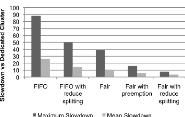
sizes using a Zipfian distribution, so that each job would have between 1 and 400 maps and a random number of re-duces between 1 andnumMaps/5. We created 20 submis-sion schedules and tested them with FIFO and fair sharing with and without copy-compute splitting, as well as fair sharing with task-killing (jobs may kill other jobs’ tasks when they are starved). Figure 8 shows response time of the workload as a whole under each scheduler. Figure 9 showsslowdownfor each job, which is defined as response time of a job in our simulation divided response time the job would achieve if it were running alone on a cluster with copy-compute splitting. There are several effects seen. Slowdowns with FIFO routinely reach 90x, showing the unsuitability of FIFO for multi-user workloads. Fair shar-ing, preemption and copy-compute splitting each cut slow-down in half. However, FIFO’s batch response time is al-ways best, even with copy-compute splitting.
5.4 Space Usage Concerns with Intermediate Data
The final complication caused by task interdependence is the issue of space used up by intermediate results on disk. Disk space is often a limited resource because in MapRe-duce there is motivation to keep as much data as possible on a cluster. For example, in a data warehouse, it is ben-eficial to keep as many months’ worth of data as possible. While many jobs use map tasks to filter a data set and thus have small map outputs, it is also possible to have maps that “explode” their input and create large amounts of in-termediate data. One example of such jobs at Facebook is map-side joins with small tables.
Hadoop already has safeguards ensure that a node’s disks won’t be filled up – the node will refuse to admit tasks that are expected to overflow its disk. However, it is possible to get “stuck” if two jobs are running concurrently and the disk becomes full before either finishes. To avoid such deadlocks, results from one job must be deleted un-til the other job completes. Any heuristic for selecting the victim job works as long as it allows some job in the cluster to monotonically make progress. Some possibilities are:
• Evict the job that was submitted latest.
0 0.2 0.4 0.6 0.8 1 1.2 FIFO FIFO + copy comp. split Fair Fair + killing tasks Fair + copy comp. split. Batch Response T ime Relative to FIFO
Figure 8: Batch response times in simulated workload.
0 10 20 30 40 50 60 70 80 90 100
FIFO FIFO with reduce splitting
Fair Fair with
preemption Fair with reduce splitting
Slowdown vs Dedicated Cluster
Maximum Slowdown Mean Slowdown
Figure 9: Averages of maximum and mean slowdowns in 20 sim-ulation runs.
• Evict the job with the least progress (% of tasks done). We note, however, that one heuristic that does not work is to evict the job using the most space. This can lead to a situation where new jobs coming into the cluster keep evicting old jobs, and no job ever finishes (for example, if there are 10 TB of free space and each job needs 10 TB, but new jobs enter just as each old job is about to finish).
Finally, we found that different scheduling disciplines can use very different amounts of intermediate space for a given workload. FIFO will use the least space because it runs jobs sequentially (its disk usage will be the maxi-mum of the required space for each job). Fair sharing may useNtimes more space than optimal whereNis the num-ber of entities sharing the cluster at a time. Shortest Re-maining Time First can useunboundedlyhigh amounts of space if the distribution of job sizes is long-tailed, because large jobs may be preempted by smaller jobs, which get preempted by even smaller jobs, and so forth for arbitrar-ily many levels. We explore tradeoffs between throughput, response time, and space usage further in Section 7.
6
Evaluation
We evaluate our scheduling techniques through mi-crobenchmarks showing the effect of particular compo-nents, and a macrobenchmark simulating a multi-user workload based on Facebook’s production workload.
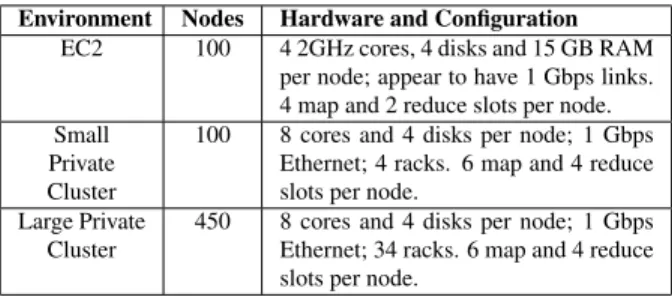
Our benchmarks were performed in three environments: Amazon’s Elastic Compute Cloud (EC2) [1], which is a commercial virtualized hosting environment, and private 100-node and 450-node clusters. On EC2, we used
“extra-Environment Nodes Hardware and Configuration
EC2 100 4 2GHz cores, 4 disks and 15 GB RAM per node; appear to have 1 Gbps links. 4 map and 2 reduce slots per node. Small
Private Cluster
100 8 cores and 4 disks per node; 1 Gbps Ethernet; 4 racks. 6 map and 4 reduce slots per node.
Large Private Cluster
450 8 cores and 4 disks per node; 1 Gbps Ethernet; 34 racks. 6 map and 4 reduce slots per node.
Table 1: Experimental environments.
large” VMs which appear to occupy a whole physical nodes. The first two environments are atypical of large MapReduce installations because they had fairly good bi-section bandwidth – the small private cluster spanned only 4 racks, and while topology information is not provided by EC2, tests revealed that nodes were able to send 1 Gbps to each other. Unfortunately, we only had access to the 450-node cluster for a limited time. We ran a recent version of Hadoop from SVN trunk, configured with a block size of 128 MB because this improved performance (Facebook uses this setting in production) and with task slots per node based on hardware capabilities. Table 1 details the hard-ware in each environment and the slot counts used.
For our workloads, we used a “loadgen” example job in Hadoop that is used in Hadoop’s included Gridmix bench-mark. Loadgen is a configurable job where the map tasks output some keepMap percentage of the input records, then the reduce tasks output akeepReducepercentage of the intermediate records. With keepMap=100% and keepReduce=100%, the job is equivalent to sort (which is the main component of Gridmix). WithkeepMap=0.1% andkeepReduce=100%, the job emulates a scan work-load where a small amount of records are aggregated (this is the second workload used in Gridmix). Making this into a map-only job emulates a “filter” job (select a subset of a large data set for further processing). We also extended loadgen to allow making mappers and reducers more CPU-intensive by performing some number of mathematical op-erations while processing each input record.
6.1 Macrobenchmark
We ran a multi-user benchmark on EC2 with job sizes and arrivals based on Facebook’s production work-load. The benchmark used loadgen jobs with random keepMap/keepReducevalues and random amounts of CPU work per record (maps took between 9s and 60s). We chose to create our own macrobenchmark instead of run-ning Hadoop’s Gridmix because, while Gridmix contains multiple jobs of multiple sizes, it does not simulate a multi-user workload (it runs all small jobs first, then all medium jobs, etc). Our benchmark, referred to as BM for short, consisted of 50 jobs of 9 sizes (numbers of maps). Table 2 shows the job size distribution at Facebook, which we grouped into 9 size bins. We picked a representative size
Bin #Maps % at Facebook Size in BM Jobs in BM
0 1-25 58% 16 29 1 25-50 9.6% 40 5 2 50-100 8.6% 80 4 3 100-200 8.4% 160 4 4 200-400 5.6% 320 3 5 400-800 4.3% 600 2 6 800-1600 2.5% 1200 1 7 1600-3200 1.3% 2400 1 8 >3200 1.7% 6400 1
Table 2: Job size distribution at Facebook and sizes and number of jobs chosen for each bin in our multi-user benchmark BM.
from each bin and submitted some number of jobs of this size to make it easier to average the performance of these jobs. For each job, we set number of reducers to 5% to 25% of the number of maps. Jobs were submitted roughly every 30s by a Poisson process, corresponding to the rate of submission at Facebook. The benchmarks ran for 30-40 minutes each (25 to submit the jobs and more to finish).
We generated three job submission schedules according to this model and compared five algorithms: FIFO and fair sharing with and without copy-compute splitting, as well as fair sharing with both copy-compute splitting and delay scheduling (all the techniques in our paper together).
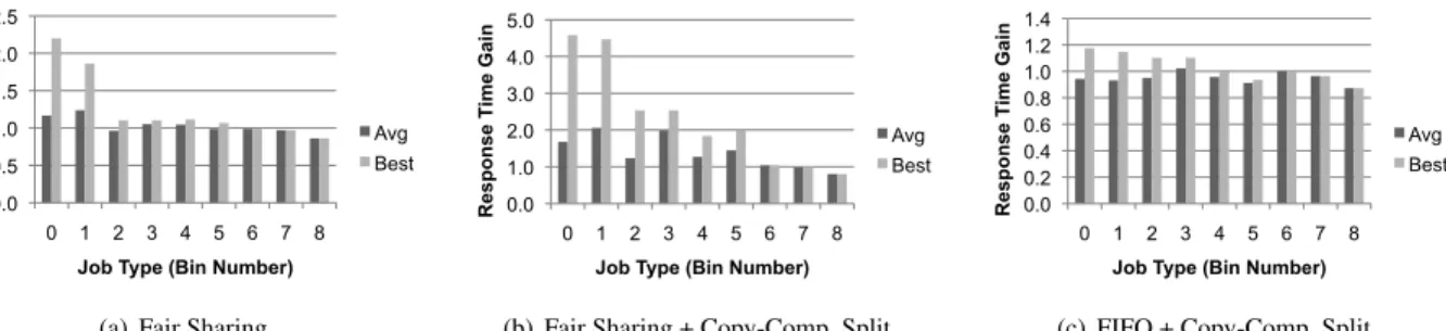
Figure 10 shows results from the “median” schedule where the average gain from our scheduling techniques was neither the lowest nor the highest. The figure shows average response time gain for each type (bin) of jobs over their response time in FIFO (e.g. a value of 2 means the job ran 2x faster than in FIFO), as well as the maximum gain for each bin (the gain of the job that improved the most). We see that fair sharing (figure (a)) can cut response times in half over FIFO small jobs, at the expense of long jobs taking slightly longer. However, some jobs are still de-layed due to reduce slot hoarding. Fair sharing with copy-compute splitting (figure (b)) provides gains of up to4.6x for small jobs, with the average gain for jobs in bins 0 and 1 being1.8-2x. Finally, FIFO with copy-compute splitting (figure (c)) yields some gains but less than fair sharing.
Adding delay scheduling does not change the response time of fair sharing with copy-compute splitting percep-tibly, so we do not show a graph for it. However, it in-creases locality to 99-100% from 15-95% as shown in Figure 11 (the values for FIFO, fair sharing, etc with-out delay scheduling were similar so we only show one set of bars). This would increase throughput in a more bandwidth-constrained environment than EC2.
In the other two schedules, average gains from fair shar-ing with copy-compute splittshar-ing for the type-0 jobs were5x and2.5x. Maximum gains were14xand10xrespectively.
6.2 Microbenchmarks
6.2.1 Delay Scheduling with Small Jobs
To test the effect of delay scheduling on locality and throughput in a small job workload, we generated a large
0.0 0.5 1.0 1.5 2.0 2.5 0 1 2 3 4 5 6 7 8 Response T ime Gain
Job Type (Bin Number)
Avg Best
(a) Fair Sharing
0.0 1.0 2.0 3.0 4.0 5.0 0 1 2 3 4 5 6 7 8 Response T ime Gain
Job Type (Bin Number)
Avg Best
(b) Fair Sharing + Copy-Comp. Split.
0.0 0.2 0.4 0.6 0.8 1.0 1.2 1.4 0 1 2 3 4 5 6 7 8 Response T ime Gain
Job Type (Bin Number)
Avg Best
(c) FIFO + Copy-Comp. Split.
Figure 10: Average and best response time gains (as a factor reduction in from FIFO) for jobs in each bin for various algorithms in multi-user benchmark. 0% 20% 40% 60% 80% 100% 0 1 2 3 4 5 6 7 8 Percent Locality Job Type
No Delay Scheduling With Delay Scheduling
Figure 11: Locality for each job bin in multi-user benchmark.
0 0.2 0.4 0.6 0.8 1
3 Maps 10 Maps 100 Maps
Normalized Running T
ime
Job Size (Number of Maps)
No Delay Scheduling With Delay Scheduling
Figure 12: Finish times in small-jobs experiment.
input set of random data and ran workloads against it in the Small Private Cluster. Each job was a map-only “scan” job which reads an input file and outputs 0.5% of the records in it, simulating “filtering” jobs common in parsing log data. We ran jobs with 3, 10 and 100 map tasks (i.e. input files of 384, 1280 or 12800 MB, since we used a block size of 128 MB). The benchmarks ran varying numbers of jobs based on the job size so as to take 10-20 minutes in total. We compared fair sharing and FIFO with and without with de-lay scheduling (T1=T2=15s). FIFO performed the same as fair sharing, so we only show two bars.
Figure 12 shows normalized running times of the work-load, while Table 3 shows locality achieved by each sched-uler. Delay scheduling increased throughput by1.2x for 3-map jobs,1.7xfor 10-map jobs, and 1.3xfor 100-map jobs, and raised data locality to at least 75% and rack lo-cality to at least 94%. The throughput gain is higher for 10-map jobs than for 100-map jobs because locality with 100-map jobs is fairly good even without delay schedul-ing. However, the gain for the smallest jobs (3 maps) is
Job Size Node/Rack Locality
with Standard Sched.
Node/Rack Locality with Delay Sched.
3 maps 2% / 50% 75% / 96%
10 maps 37% / 98% 99% / 100%
100 maps 84% / 99% 94% / 99%
Table 3: Locality in small-jobs experiment.
0 10 20 30 40 50
5 Jobs 10 Jobs 20 Jobs 50 Jobs
T
ime to Run W
orkload (min)
Without Delay Scheduling With Delay Scheduling
Figure 13: Finish times in sticky slots experiment.
lower than for 10-map jobs, because at small job sizes, job initialization becomes a bottleneck in Hadoop.
Interestingly, virtually all the gains in the 10-map and 100-map cases are due to moving from rack-local to node-local tasks; rack node-locality was good even without delay scheduling because our cluster contained only 4 racks and each file is replicated on 2 racks in Hadoop. We expect performance gains to be higher in a larger cluster.
6.2.2 Delay Scheduling with Sticky Slots
As explained in Section 4.1, sticky slots do not normally occur in Hadoop due to a counting bug. We tested a ver-sion of Hadoop with this bug fixed to quantify the effect of sticky slots. We ran this test in the EC2 environment. We generated a large 180-GB data set (2 GB per node), submit-ted between 5 and 50 concurrent scan jobs on it, and mea-sured the time to finish all jobs and the locality achieved. Figures 13 and 14 show the results with and without delay scheduling (withT1=10s). Delay scheduling improves by throughput by1.1xfor 10 concurrent jobs,1.6xfor 20 con-current jobs, and2xfor 50 concurrent jobs. It also brings locality from 90-27% to 99-100%.
0% 20% 40% 60% 80% 100%
5 Jobs 10 Jobs 20 Jobs 50 Jobs
Percent Local Maps
Without Delay Scheduling With Delay Scheduling
Figure 14: Node locality in sticky slots experiment.
6.2.3 Impact of Delay Scheduling on Response Time
We measured the response time of a small 16-map / 1-reduce job (scanning 2 GB and sending 0.1% of the data to the reduce task) with and without delay scheduling (10s) on EC2 to quantify the impact on response time. We ran the job eight times under each condition. Running alone, the job took32-37s, with a mean of35.4s. With delay schedul-ing, the job took32-38swith a mean again of35.4s. The difference in response time was not statistically significant, but locality improved from25%to100%.
6.2.4 IO-Rate Biasing
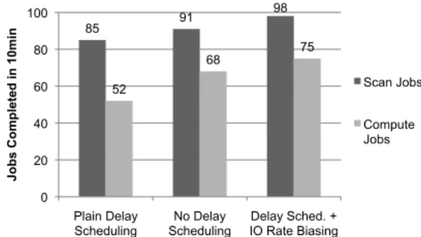
To evaluate IO-rate biasing, we generated a hotspot situa-tion on EC2 as follows. We created a 2 GB file with 3x replication as input. We then had 20 simulated “workers” submit jobs on this file for 10 minutes. Ten workers sub-mitted compute-intensive jobs which performed a number of mathematical operations after reading each input record, taking about 36s per map task, while ten others submitted IO-bound scan jobs as in the previous experiments, which take 9s per map task. Each worker repeatedly submitted a job and waited for it to finish. After 10 minutes, we counted total jobs completed. We tested this workload us-ing three algorithms (all under fair sharus-ing): untuned delay scheduling withT1=10s delay for both types of jobs, no delay scheduling, and delay scheduling with IO-rate bias-ing (T1=10s for scans and 0s for compute jobs).
Figure 15 shows the throughput for each algorithm. Un-tuned delay scheduling achieved the worst throughput and response times, because both compute and scan jobs would wait up to 10s to run on a contended data-local local slot, and then half the time a compute job would take the slot and hold it for 36s (whereas a scan job would only take 10s) – this is an environment where the throughput analy-sis at the start of Section 4.3.2 breaks down because there is a hotspot. Turning delay scheduling off led to better performance simply because tasks could get launched ear-lier. However, using delay scheduling with IO-rate bias-ing (delaybias-ing only the scan jobs) led to the best perfor-mance because the scans would almost always get data-local slots. Compute jobs also ran faster due to a combina-tion of less data being sent across the network and possibly
85 91 98 52 68 75 0 20 40 60 80 100 Plain Delay Scheduling No Delay Scheduling Delay Sched. + IO Rate Biasing
Jobs Completed in 10min
Scan Jobs Compute Jobs
Figure 15: Throughputs in IO-rate biasing experiment.
less CPU contention on the machines serving the blocks. The throughput gain with IO-rate biasing over no delay scheduling was8%for scans and10%for compute jobs, while the gain over untuned delay scheduling was15%for scans and44%for compute jobs.
6.2.5 Copy-Compute Splitting in Single Job
In addition to the experiments in Section 6.1 that mea-sure throughput gain from copy-compute splitting in a multi-user workload, we ran an experiment demonstrat-ing a gain in a sdemonstrat-ingle-user, sdemonstrat-ingle-job workload. Unfor-tunately, Hadoop’s copy tasks are fairly CPU-intensive because they perform large amounts of memory copies when merging map outputs, so there is little gain from copy-compute splitting unless the network bandwidth is very limited (copy tasks compete with compute tasks with CPU). The largest cluster we had access to was a 450-node cluster with nodes distributed on 34 racks. On this cluster, we ran a synthetic job with an identity map function and a compute-intensive reduce function. The job had 1.8 TB of input data, 14624 map tasks and 5000 reduce tasks. The reduces ran in three waves because the cluster was config-ured with 1800 reduce slots (four per node). The job took on average12.9minutes with standard reduce scheduling and11.8minutes with copy-compute splitting, a9%gain. We expect the gain to be higher in larger clusters (where bi-section bandwidth is more limited) or with a more efficient implementation of copy tasks.
6.2.6 Batch Response Time with Fair Sharing vs FIFO
We illustrate the throughput reduction for fair sharing over FIFO in MapReduce explained in Section 5.3 using a work-load with 5 jobs running either in FIFO or fair sharing on the EC2 environment. Each job read 100 GB of data. The job’s maps produced 200 GB of output total (i.e. doubling the size of their input), which was passed on to 190 reduce tasks. The reduce tasks outputted only a small result set but also performed expensive mathematical computations for each input record. We repeated the experiment three times. Fair Sharing took26.2±0.3minutes to complete the workload, while FIFO took 22.1±0.2minutes. This corresponds to19%higher throughput with FIFO.
7
Discussion
Underlying our work is a classic tradeoff between utiliza-tion and user isolautiliza-tion. In considering how to provision data-intensive computing infrastructure, there is a spec-trum between having a separate cluster per user, which pro-vides great isolation but poor utilization, and having a sin-gle FIFO cluster, which provides great utilization but no isolation. Our work enables a sweet spot on this spectrum – sharing a large cluster efficiently while giving each user response times equivalent to a small private cluster. This lets interactive queries and production jobs run on a shared cluster. Furthermore, the data consolidation in a shared cluster enables applications that would be impossible to run on smaller private clusters with partitioned data. To-gether, these factors let an organization extract more value from its data per dollar of computing infrastructure.
We identified two aspects of the data-intensive cluster computing setting that pose problems to sharing: data lo-cality and interdependent tasks. Although we worked in the setting of MapReduce, these problems are relevant in any cluster computing system that uses DAGs of processes to perform computations, such as Dryad [20]. Any such system needs to place tasks on nodes that contain their in-put, and risks experiencing the head-of-line scheduling and sticky slot problems we described. Similarly, tasks that must collect data from multiple other tasks before perform-ing a computation are common. Our delay schedulperform-ing and copy-compute splitting techniques can improve throughput and response time in any data flow based system.
We divide our discussion into three parts. Section 7.1 describes lessons for making cluster computing systems sharable. Section 7.2 analyzes tradeoffs between schedul-ing disciplines in MapReduce. Finally, we present other scheduling issues we considered at Facebook in Section 7.3.
7.1 Lessons For Multi-User Cluster Scheduling
Because of the significant benefits of shared clusters when there is shared data, we believe that cluster computing sys-tem designers should consider making multi-user support a primary goal. Our work shows that, as long as jobs are composed of small independent tasks, it is possible to iso-late users while utilizing a cluster efficiently. We identify four principles that help achieve this goal:
1. Make tasks smallin length and in resource consump-tion. Having short tasks lets new jobs start up quickly. Limiting resource use by each task (e.g. making tasks single-threaded and having multiple slots per node) fur-ther increases scheduling opportunities. This principle is similar to making time slices small in a cooperative multiprocessing OS. Interestingly, MapReduce initially used small independent tasks for fault tolerance, to vir-tualize where and when a task runs. This same virtual-izability lets us achieve high scheduler responsiveness.
2. Delimit tasks into pieces with orthogonal resource requirementsto have separate admission control for each piece. Using separate processes is not necessary; an admission control check as in CPAC can be enough.
3. When tasks must be long, make them preemptable.
For example, it would be possible to pause copy tasks to better control load on slaves. This is similar to mak-ing processes preemptable in a time-slicmak-ing OS. 4. Be ready to sacrifice some isolation for throughput,
as illustrated by delay scheduling.
7.2 Scheduling Tradeoffs in MapReduce
We explore MapReduce scheduling tradeoffs in Table 4 by comparing four scheduling disciplines along four axes. The disciplines we compare are FIFO, fair sharing, short-est job first, and multi-level queueing (separate queues for small and large jobs, with weighted fair sharing between the queues). The axes we compare on are average response time, batch response time (response time for a group of jobs submitted together), intermediate space, and user iso-lation (defined as the ability to provide worst-case per-formance comparable to owning a smaller private cluster regardless of user workload). Intermediate space is not usually considered in compute-oriented cluster scheduling problems but matters in MapReduce because there is an in-centive to store as much data as possible on a cluster. We summarize the three most interesting results:
1. Batch response times can suffer in disciplines other than FIFO because maps may finish later and therefore pipelining between map and reduce tasks decreases. For this reason, we plan to support FIFO and multi-level queueing within pools in our scheduler.
2. FIFO uses the least space (no more than needed by the largest job), as explained in Section 5.4, while disci-plines that must to let multiple jobs coexist need more space. Space usage is unboundedly bad with Shortest Job First because arbitrarily many jobs may stay in the system for an arbitrarily long time.
3. Only fair sharing provides isolation (even in multi-level queues, one user’s jobs may be delayed by other users). Even though fair sharing is suboptimal for response time and space usage, we found that user isolation trumps these concerns by creating an environment where users can launch jobs at any time without fear of interference. In fact, at Facebook, average job sizesdecreasedwhen we in-troduced fair sharing, because users preferred submitting small queries that sample a data set and return within min-utes to large jobs that scan the entire data set but take tens of minutes. In other words, user isolation increased “in-sight throughput” (useful analyses per second). One final benefit is that launching jobs right away lets users find bugs faster: without fair sharing, a user who submits a job a buggy map or reduce function will not find out until the job reaches the head of the queue and gets launched.
Discipline Batch Response Time Average Response Time Intermediate Space User Isolation
First In First Out best bad unless job sizes are similar best none Fair Sharing can suffer boundedly bad boundedly bad best
Shortest Job First can suffer bestbut starves long jobs unboundedly bad none
Multi-Level Queuing can suffer good boundedly bad some
Table 4: Tradeoffs between various scheduling disciplines in MapReduce.
7.3 Other Scheduling Issues
Through our work developing a job scheduler for Hadoop, we identified several scheduling concerns that we do not explore in this paper, but plan to study in future work: Code Locality: Running multiple tasks from a job on the same node is beneficial because it amortizes the cost of copying the job’s code to this node. Furthermore, Hadoop lets tasks from the same job reuse JVM instances, reducing startup costs. Fixing the Hadoop bug that prevents sticky slots from happening and using delay scheduling may im-prove code locality by letting a job run on a node until it exhausts its input data, then move on to other nodes. The issue of maximizing “code locality” is similar to affin-ity scheduling in multiprocessor operating systems, where we attempt to pin a thread to a processor for as long as possible; however, we expect that in the MapReduce set-ting, data locality will be the primary consideration in task placement, while code locality will be secondary.
Slave Load Management: When jobs with different
re-source requirements (especially memory needs) coexist, it would be beneficial to use a more elaborate mechanism for load management on slave nodes than task slots, as discussed in Section 2. Work in [5] allows Hadoop to avoid thrashing memory on a slave when some tasks have high requirements by using less than the full number of slots. However, another issue that can happen is starva-tionof memory-intensive jobs if jobs with smaller mem-ory requirements keep taking slots. Task-killing in our scheduler (Section 3.2) can be used to make room for the memory-intensive job, but we also plan to investigate a de-lay scheduling technique where a high-memory job picks a number of nodes to run on and waits for enough tasks on each of them to complete. In addition, we will need to change our fairness/accounting model so that a job taking up more memory counts as having filled more “slots”.
8
Related Work
Fair Sharing: A plethora of fair sharing algorithms have been developed in the networking and OS domains to pro-vide isolation and statistical multiplexing among flows and computation tasks [8, 13, 17, 24]. Many of these schedulers have been extend to the hierarchical setting, where each interior node in the hierarchy share bandwidth or CPU re-sources across its children [14, 18, 21, 23]. While these al-gorithms are sophisticated and scalable, they do not deal with data locality, as they share only one resource, and in general they ignore interdependencies between tasks/flows.
HPC: Schedulers for HPC clusters, like Torque [12], sup-port job priority and resource-consumption-aware schedul-ing. However, the HPC jobs they schedule run on a fixed number of machines which communicate through a mech-anism like MPI. MapReduce jobs are elastic, so we can change allocations over time. HPC jobs are also CPU-bound, so there is less need for node-level data locality. Grids: Grid schedulers like Condor [22] support locality constraints, but usually at the level of geographic sites, because the jobs are still more compute-intensive than MapReduce. Recent work in grid scheduling [15] also pro-poses replicating data to multiple geographic sites in re-sponse to jobs being launched. This is similar to increasing a file’s replication level in Hadoop.
Parallel Databases: Like MapReduce, parallel databases run data-intensive workloads on a distributed system. The main aspects differentiating MapReduce from these sys-tems are the scale and use of commodity hardware in MapReduce, and the MapReduce execution strategy of small independent tasks instead of long-running pipelined queries. The largest parallel databases, like Teradata, can run on up to 1024 dual-core nodes, but use external stor-age arrays and proprietary high-speed interconnects with high bisection bandwidth [9, 11]. This makes data local-ity less of a concern than in Hadoop (any node in Ter-adata can access any disk if the primary node assigned to that disks fails), but increases system costs. In con-trast, Hadoop can run on 10000-core clusters of commodity machines connected by Ethernet [2], but this necessitates careful management of data locality. In addition, paral-lel database queries are generally long-running processes that pipeline data between operators rather than short tasks like Hadoop’s, reducing opportunity for high-granularity scheduling. A single “monster query” can take up the en-tire system [9]. Admission control is used to avoid over-subscribing resources [7], which means that queries may need to wait in a queue to be executed. To avoid starving interactive queries, resources may be explicitly reserved for them [7], but this leads to underutilization when there are no interactive queries running. In contrast, our Hadoop scheduler can use all resources towards batch jobs and re-assign slots quickly when interactive jobs are submitted.
9
Conclusion
While MapReduce has proven a popular execution model for large batch jobs, recently, many organizations have started to share their MapReduce (Hadoop) clusters among
multiple users, which run a mix of batch and short in-teractive jobs. To enable this use model, we have pro-posed FAIR, a fair scheduler that provides isolation, guarantees a minimum share to each user (job), and achieves statistical multiplexing. During its initial deploy-ment, we have identified two aspects of MapReduce— data locality and task interdependence—which consider-ably hurt FAIR’s throughput. To address this issue we have developed two simple yet robust techniques: delay scheduling and copy-compute splitting. Using a wide ar-ray of experiments we have shown that FAIR achieves iso-lation, low response time, and high throughput.
10
Acknowledgements
We would like to thank the Hadoop teams at Yahoo! and Facebook for the discussions based on practical experience that guided this work. We are also grateful to Joe Heller-stein and Hans Zeller for their pointers to related work in database systems. This res
![Figure 1: Data flow in MapReduce. Figure from [4].](https://thumb-us.123doks.com/thumbv2/123dok_us/650096.2578402/4.918.468.818.79.325/figure-data-flow-mapreduce-figure.webp)