SFB
823
Nonparametric tests for
constant tail dependence with
an application to energy and
finance
Discussion Paper
Axel Bücher, Stefan Jäschke, Dominik Wied
Nonparametric tests for constant tail dependence with
an application to energy and finance
Axel B¨
ucher
aUniversit´e catholique de Louvain & Ruhr-Universit¨at Bochum
Stefan J¨
aschke
∗,bRWE Supply & Trading GmbH
Dominik Wied
cTechnische Universit¨at Dortmund
August 13, 2013
Abstract
The present paper proposes new tests for detecting structural breaks in the tail dependence of multivariate time series using the concept of tail copulas. To obtain asymptotic properties, we derive a new limit result for the sequential empirical tail copula process. Moreover, consistency of both the tests and a change-point estima-tor are proven. We analyze the finite sample behavior of the tests by Monte Carlo simulations. Finally, and crucial from a risk management perspective, we apply the new findings to datasets from energy and financial markets.
Keywords: Change-point detection, Multiplier bootstrap, Tail dependence, Weak convergence
JEL classification: C12, C14, C32, C58, G32
This work has been supported in part by the Collaborative Research CenterStatistical Modelling of
Nonlinear Dynamic Processes(SFB 823, projects A1 and A7) of the German Research Foundation (DFG)
and by the IAP research network Grant P7/06 of the Belgian government (Belgian Science Policy). ∗Corresponding author.
aUniversit´e catholique de Louvain, Institut de statistique, Voie du Roman Pays 20, 1348 Louvain-la-Neuve, Belgium, Email: [email protected].
bRWE Supply & Trading GmbH, Risk Valuation, Altenessener Str. 27, 45141 Essen, Germany, Email: [email protected].
cTechnische Universit¨at Dortmund, Fakult¨at Statistik, Vogelpothsweg 87, 44221 Dortmund, Germany, Email: [email protected].
1. Introduction
Modeling and estimating stochastic dependencies has attracted increasing atten-tion over the last decades in various fields of applicaatten-tions, including mathematical finance, actuarial science or hydrology, among others. Of particular interest, espe-cially in risk management, is a sensible quantitative description of the dependence between extreme events, commonly referred to as tail dependence; see for example Embrechts et al. (2003). A formal definition of this concept is given in Section 2 below.
In applications, tail dependence is often assessed by fitting a parametric copula family to the data and by subsequently extracting the tail behavior of that particu-lar copula. Examples can be found in Breymann et al. (2003) and Malevergne and Sornette (2003), among others. More robust methods are based on the assumption that the underlying copula is an extreme-value copula. The class of these copulas can be regarded as a nonparametric copula family indexed by a function on the unit simplex (Gudendorf and Segers, 2010). Since the copula is a rather general measure for stochastic dependence, the estimation techniques for both of the lat-ter approaches are usually based on the entire available dataset (see, for instance, Genest et al. (1995); Chen and Fan (2006) for parametric families or Genest and Segers (2009) for extreme-value copulas). However, due to the fact that the center of a distribution does not contain any information about the tail behavior, these techniques might in general yield biased estimates for the tail dependence. We refer to Frahm et al. (2005) for a more elaborated discussion of this issue. In order to circumvent the problem and to obtain estimators that are robust with respect to deviations in the center of the distribution, there are basically two important approaches: either one could extract the tail dependence from subsamples of block maximal data, for which extreme-value copulas provide a natural model (McNeil et al., 2005, Section 7.5.4), or one could rely on extreme-value techniques some of which are presented in Section 2 below. Applications of these procedures can be found in Breymann et al. (2003); Caillault and Gu´e´egan (2005); J¨aschke et al. (2012); J¨aschke (2012), among others.
Most of the aforementioned applications to time series data are based on the implicit assumption that the tail dependence remains constant over time. Whereas nonparametric testing for constancy of the whole dependence structure, as for in-stance measured by the copula, has recently drawn some attention in the literature (Remillard, 2010; Busetti and Harvey, 2011; Kr¨amer and van Kampen, 2011; van Kampen and Wied, 2012; Kojadinovic and Rohmer, 2012; B¨ucher and Ruppert, 2013), there does not seem to exist a unified approach to testing for constancy of the tail dependence. It is the main purpose of the present paper to fill this gap. Our proposed testing procedures are genuine extreme-value methods depending only on the tails of the data and are hence robust with respect to potential (non-)constancy of the dependence between the centers of the distributions. In particular, the pre-sented tests do not rely on the assumption of a constant copula throughout the sample period.
Our procedures are based on new limit results for the sequential empirical tail copula process, formally defined in Section 3.1. We derive its asymptotic distri-bution under the null hypothesis and propose several variants to approximate the required critical values. When restricting to the case of testing for constancy of the simple tail dependence coefficient, the limiting process can be easily transformed
into a Brownian bridge. In this case, the asymptotic critical values of the tests can be obtained by direct calculations or simulations. In the more complicated case of testing for constancy of the whole extremal dependence structure as measured by the tail copula, we propose a multiplier bootstrap procedure to obtain approximate asymptotic quantiles. The finite-sample performance of all proposals is assessed in a simulation study, which reveals accurate approximations of the nominal level and reasonable power properties.
We apply our methods to two real datasets. The first application revisits a recent investigation in J¨aschke (2012) on the tail dependence between WTI and Brent crude oil spot log-returns, which is based on the implicit assumption that the tail dependence remains constant over time. Our testing procedures show that this assumption cannot be rejected. The second application concerns the tail de-pendence between Dow Jones Industrial Average and the Nasdaq Composite time series around Black Monday on 19th of October 1987, it reveals a significant break in the tail dependence. However, our results do not show clear evidence for the hypothesis that this break takes place at the particular date of Black Monday.
The structure of the paper is as follows: in Section 2, we briefly summarize the concept of tail dependence and corresponding nonparametric estimation techniques. The new testing procedures for constancy of the tail dependence are introduced in Section 3. In particular, we derive the asymptotic distribution of the sequential empirical tail copula process, propose a multiplier bootstrap approximation of the latter and show consistency of various asymptotic tests. Additionally, we deal with the estimation of change-points in case the null hypothesis is rejected and pro-pose a data-adaptive way for the necessary parameter choice, common to inference methods in extreme-value theory. A comprehensive simulation study is presented in Section 4, followed by the two elaborate empirical applications in Section 5. All proofs are deferred to an Appendix.
2. The concept of tail dependence and its
nonparametric estimation
Let (X, Y) be a bivariate random vector with continuous marginal cumulative dis-tribution functions (c.d.f.s) F and G. Lower or upper tail dependence concerns the tendency that extremely small or extremely large outcomes ofX and Y occur simultaneously. Simple, widely used and intuitive scalar measures for these ten-dencies are provided by the well-established coefficients of tail dependence (TDC), defined as
λL= lim
t&0P{F(X)≤t|G(Y)≤t}, λU = limt%1P{F(X)≥t|G(Y)≥t} (1)
see for instance Joe (1997); Frahm et al. (2005), among others.
It is well-known that the joint c.d.f.Hof (X, Y) can be written in a unique way as
H(x, y) =C{F(x), G(y)}, x, y∈R, (2) where the copulaC is a c.d.f. on [0,1]2 with uniform marginals. Elementary
calcu-lations show that the conditional probabilities in (1) can be written as λL= lim t&0 C(t, t) t , λU = limt&0 C(t, t) t ,
whereC denotes the survival copula of (X, Y). Therefore, the coefficients of tail dependence can be regarded as directional derivatives ofC orC at the origin with direction (1,1). Considering different directions, we arrive at the so-called lower tail copulas, defined for any (x, y)∈E= [0,∞]2\ {(∞,∞)} by
ΛL(x, y) = lim t&0 C(xt, yt) t , ΛU(x, y) = limt&0 C(xt, yt) t , (3)
see Schmidt and Stadtm¨uller (2006). Note that the upper tail copula of (X, Y) is the lower tail copula of (−X,−Y), whence there is no conceptual difference between upper and lower tail dependence.
Several variants of tail copulas have been proposed in the literature on mul-tivariate extreme-value theory. For instance, L(x, y) = x+y−ΛU(x, y) denotes
the stable tail dependence function, see, e.g., de Haan and Ferreira (2006). The function A(t) = 1−ΛU(1−t, t), which is simply the restriction of L to the unit
sphere with respect to thek · k1-norm, is called Pickands dependence function, see
Pickands (1981). All these variants are one-to-one and are known to characterize the extremal dependence of X and Y, see de Haan and Ferreira (2006). In the present paper we restrict ourselves to the case of tail copulas.
Nonparametric estimation ofLand Λ has been addressed in Huang (1992); Drees and Huang (1998); Einmahl et al. (2006); de Haan and Ferreira (2006); B¨ucher and Dette (2011); Einmahl et al. (2012) for i.i.d. samples (Xi, Yi)i∈{1,...,n}. For instance, in the case of lower tail copulas, the considered estimators are slight variants, differing only up to a term of uniform order O(1/k), of the function
(x, y)7→ 1 k n X i=1 1Ri≤kx, Si ≤ky (4)
where Ri (resp. Si) denotes the rank of Xi (resp. Yi) among X1, . . . , Xn (resp.
Y1, . . . , Yn), and wherek =kn → ∞ denotes an intermediate sequence to be
cho-sen by the statistician. Under suitable assumptions on kn and on the speed of
convergence in (3) the estimators are known to be √kn-consistent. Additionally,
under certain smoothness conditions on Λ, the corresponding process√kn( ˆΛ−Λ)
converges to a Gaussian limit process.
3. Testing for constant tail dependence
3.1. Setting and test statistics Let (Xi, Yi)i∈{1,...,n} be an independent
sequence of bivariate random vectors with joint c.d.f.Hi and identical continuous
marginal c.d.f.s F and G, respectively. According to Sklar’s Theorem, see (2), we can decompose
where Ci(u, v) = P(Ui ≤u, Vi ≤v) with Ui =F(Xi) and Vi =G(Yi). We assume
that the corresponding lower tail copulas Λi(x, y) = lim
t→∞tCi(x/t, y/t) (5)
exist for all (x, y)∈E= [0,∞]2\ {(∞,∞)} and all i= 1, . . . , n.
The assumption of i.i.d. marginal time series may appear somewhat restrictive. Nonetheless, in the literature on testing for constant copulas, it can be considered as a common practice, see for instance Busetti and Harvey (2011); Remillard (2010); van Kampen and Wied (2012); Kojadinovic and Rohmer (2012). In Section 5, the role of (Xi, Yi) will be played by the unobservable, serially independent innovations
of popular time series models such as AR or GARCH processes. In these cases, we will apply the proposed tests to the observable, standardized residuals (obtained by univariate filtering) and consider these residuals asalmost i.i.d. Our extensive simulation study in Section 4 indicates that the additional estimation step does not influence the asymptotic behavior of our test statistics, i.e., the asymptotic distribution of the estimator based on residuals is the same as the one based on the unobservable, serially independent innovations. Note that this observation is supported by the results in Chen and Fan (2006); Remillard (2010); Chan et al. (2009), where it is shown that the asymptotic distributions of both semi- and non-parametric estimators in copula models are not influenced by marginal filtering.
It is our aim to develop tests for detecting changes in the tail dependence, i.e., to test for
H0Λ: there exists Λ>0 such that Λi ≡Λ for all i= 1, . . . , n
against alternatives involving the non-constancy of Λi. A special case of this null
hypothesis is given by considering the conventional lower tail dependence coefficient
λi = Λi(1,1). The corresponding null hypothesis reads as
H0λ : there exists λ >0 such thatλi=λfor all i= 1, . . . , n.
In order to motivate our test statistics, let us first recapitulate the empirical tail copula from Schmidt and Stadtm¨uller (2006) as the basic nonparametric esti-mator for Λ underH0Λ, see also (4) and the corresponding citations. Replacing the unknown copula in (5) by the empirical copula Cn, it is defined as
ˆ Λn(x, y) = n kCn kx n , ky n = 1 k n X i=1 1Uˆi ≤kx/n,Vˆi≤ky/n , (6)
where ( ˆUi,Vˆi) denotepseudo-observations from the copulaC, defined by
ˆ Ui = n n+ 1Fn(Xi), Vˆi = n n+ 1Gn(Yi),
withFnandGndenoting the marginal empirical c.d.f.s. Additionally,k=kn→ ∞,
k=o(n), represents a sequence of parameters discussed in detail below. The ratio
k/ncan be interpreted as the fraction of data that one considers asbeing in the tail and thus taken into account to estimate the tail dependence in Equation (6). Under suitable regularity conditions some of which are given in the subsequent Section 3.2, it is known that ˆΛn is
√
tail copula process (x, y)7→√k{Λˆn(x, y)−Λ(x, y)}converges weakly to a Gaussian
limit process.
Now, in order to test for H0Λ, it is natural to consider a suitable sequential version of ˆΛn. We define ˆ Λ◦n(s, x, y) = 1 k bnsc X i=1 1 ˆ Ui≤kx/n,Vˆi ≤ky/n
as the sequential empirical tail copula. Under H0Λ, ˆΛ◦n should be regarded as an estimator for Λ◦(s, x, y) = sΛ(x, y). Note that ˆΛ◦n(1, x, y) = ˆΛn(x, y). The crucial
quantity for all test procedures in this paper is now given by the corresponding sequential empirical tail copula process {Gn(s, x, y), s∈[0,1],(x, y)∈E} with
Gn(s, x, y) =
√
knΛˆ◦n(s, x, y)−sΛˆ◦n(1, x, y)o.
Some simple calculations show that, fors∈(0,1),Gn can be written as
Gn(s, x, y) = √ k{s(1−s)} 1 ks bnsc X i=1 1 ˆ Ui≤kx/n,Vˆi≤ky/n − 1 k(1−s) n X i=bnsc+1 1 ˆ Ui≤kx/n,Vˆi ≤ky/n .
Since ks ≈ bksc, ns ≈ bnsc and k/n ≈ bksc/bnsc for any s ∈ (0,1), the two summands in the brackets on the right-hand side can be interpreted as (slightly adapted) empirical tail copulas of the subsamples (X1, Y1), . . . ,(Xbnsc, Ybnsc) and (Xbnsc+1, Ybnsc+1), . . . ,(Xn, Yn), respectively, with corresponding sequence of
pa-rameters k0 = bksc and k00 = bk(1−s)c. Under H0Λ, one would expect that the difference between these two estimators converges to 0. Therefore, any statistic that can be interpreted as a distance betweenGnand the function being constantly equal
to 0 is a reasonable candidate for a test statistic for the null hypothesis. A simula-tion study similar to one presented in Secsimula-tion 4 showed that a Cram´er-von Mises functional yields to the best finite-sample performance, which is why we restrict ourselves to this case in the subsequent presentation. Consequently, in case of the simple null hypothesis H0λ, we propose the test statistic
Sn:={Λˆ◦n(1,1,1)}−1 Z 1
0
{Gn(s,1,1)}2ds (7)
and to reject the null hypothesis wheneverSnis larger than an appropriate critical value to be determined later on.
For the construction of a test for the null hypothesis H0Λ, we make use of the fact that, by homogeneity, the lower tail copula is uniquely determined by its values on the sphereS(c) ={x∈[0,∞)2:kxk=c}, wherek · kdenotes an arbitrary fixed norm on R2 and where c > 0 is an arbitrary fixed constant. The most popular
choice in bivariate extreme value theory is c = 1 together with the k · k1-norm resulting in the function B : [0,1]→ [0,1/2] : t 7→ B(t) = Λ(1−t, t). Note that
In order to test for overall constancy of Λi it is sufficient to test for constancy
of Λion some sphereS(c). In Section 3.5, we will propose a data-adaptive procedure
for the choice of the parameterk, which will suggest to use a sphere that contains the point (1,1). For that reason, we introduce the following test statistic
Tn:= Z 1 0 Z 1 0 {Gn(s,2−2t,2t)}2dtds,
whose support corresponds to the k · k1-norm and c = 2, and let H0Λ again be
rejected whenTn is larger than an appropriate critical value.
In order to determine the critical values, we will derive the asymptotic null distributions of the tests in the next subsection. For both statistics, they will rely on a limit result for the sequential empirical tail copula process.
3.2. Asymptotic null distributions LetB∞([0,1]×E) denote the space of
all functions f : [0,1]×E → R which are uniformly bounded on every compact subset of [0,1]×E (here and throughout, we understand E = [0,∞]2 \ {(∞,∞)}
as the one-point uncompactification of the compact set [0,∞]2), equipped with the
metric d(f, g) = ∞ X m=1 2−m(kf −gkSm∧1),
wherea∧b= min(a, b), where the sets Sm are defined as Sm= [0,1]×Tm with
Tm= [0, m]2∪({∞} ×[0, m])∪([0, m]× {∞})
and where k · kS denotes the sup-norm on a set S. Note that convergence with
respect todis equivalent to uniform convergence on each Sm.
In the following we are going to show weak convergence ofGn as an element of
the metric space (B∞([0,1]×E), d). Similar as in related references on the estimation
of tail copulas (see Section 2), we have to impose several regularity conditions. First, we need a second order condition quantifying the speed of convergence in (5) uniformly in iand (x, y).
Assumption 3.1. We haveΛi6≡0 and
Λi(x, y)−tCi(x/t, y/t) =O(B(t)), t→ ∞, (8)
uniformly on {(x, y) ∈ [0,1]2 : x +y = 1} (and hence uniformly on each Tm)
and uniformly in i ∈ N, where B : [0,∞) → [0,∞) denotes a function satisfying limt→∞B(t) = 0.
Second, the following conditions have to be imposed on the sequence k=kn. Assumption 3.2. For some α > 0, the non-decreasing sequence k = kn → ∞
satisfies the conditions (a) kn/n↓0, (b)
√
knB(n/kn) =o(1), (c) lim sup
n→∞ kbnδc/kn ≤δα
as ntends to infinity, where (c) has to hold for any δ∈(0,1).
Condition (a) is needed anyway to define a meaningful estimator. Condition (b) allows to control appearing bias terms in the non-sequential empirical tail copula
process, see also Schmidt and Stadtm¨uller (2006) and B¨ucher and Dette (2011). Finally, Condition (c), which can be regarded as very light, will allow to transfer the results from the non-sequential to the sequential setting.
With these assumptions we can now state the main result of our paper.
Proposition 3.3. Suppose that Assumptions 3.1 and 3.2 hold. Then, under H0Λ,
Gn GΛ in (B∞([0,1]×E), d),
whereGΛ(s, x, y) =BΛ(s, x, y)−sBΛ(1, x, y). Here,BΛis a tight centered Gaussian
process with continuous sample paths and with covariance structure
E[BΛ(s1, x1, y2)BΛ(s2, x2, y2)] = (s1∧s2)Λ(x1∧x2, y1∧y2).
As stated above, Assumption 3.2 (b) is needed to control bias terms occurring when estimating Λ by ˆΛn. As the processGndoes not involve the true tail copula Λ,
the assertion of Proposition 3.3 actually holds if (b) is replaced by a quite technical, but less restrictive assumption, see Remark A.2 in the appendix. However, as an application of the proposed test procedures in this paper will usually be followed by the application of estimation techniques relying on (b), we do not feel that imposing this condition is too restrictive.
Proposition 3.3 immediately yields the asymptotic null distributions ofSnandTn. Proposition 3.4. Suppose that Assumptions 3.1 and 3.2 hold. Then, under H0Λ,
Sn S = Z 1
0
{B(s)}2ds,
where B is a one-dimensional standard Brownian bridge, and Tn T = Z 1 0 Z 1 0 {GΛ(s,2−2t,2t)}2dtds,
where GΛ is defined in Proposition 3.3.
Note that, in fact, the weak convergence ofSncan be derived under a relaxation of H0Λ, as it suffices that Λi(x, y) 6≡ 0 exists and is constant in time in an open
neighborhood of (1,1). This is, however,a bit more than assumed in H0λ.
Since the limiting distribution for Sn in Proposition 3.4 is pivotal, we directly obtain an asymptotic levelα test for H0λ.
TDC-Test 1. Reject H0λ for Sn≥q1C−α, whereqC1−α denotes the (1−α)-quantile
of the Cram´er-von Mises distribution, the latter being defined as the distribution of the random variableR1
0{B(s)} 2ds.
In order to derive critical values for the test based on Tn, some more effort is needed. Its limiting distribution in Proposition 3.4 is not pivotal and cannot be easily transformed to a distribution which is independent of Λ. Therefore, we propose an appropriate bootstrap approximation for GΛ which will also allow for
the definition of an alternative test forH0λ.
Let B ∈ N be a large integer and let ξ1(1), . . . , ξ
(1)
n , . . . , ξ1(B), . . . , ξ
(B)
n be an
in-dependent sequence of n×B i.i.d. non-negative random variables with mean and variance 1 which are independent of the data (X1, Y1), . . . ,(Xn, Yn) and possess
let ¯ξn(b) = n−1Pni=1ξ
(b)
i denote the arithmetic mean of ξ
(b)
1 , . . . , ξ
(b)
n . Similar in
spirit as in B¨ucher and Dette (2011) we define, for any (s, x, y) ∈ [0,1]×E and
b∈ {1, . . . , B}, Gn,ξ(b)(s, x, y) =Bn,ξ(b)(s, x, y)−sBn,ξ(b)(1, x, y), where Bn,ξ(b)(s, x, y) = √ k{Λˆ◦n,ξ(b)(s, x, y)−Λˆ ◦ n(s, x, y)} and ˆ Λ◦n,ξ(b)(s, x, y) = 1 k bnsc X i=1 ξ(ib) ¯ ξ(nb) 1( ˆUi ≤kx/n,Vˆi ≤ky/n).
The following proposition states that, for large n, Gn,ξ(1), . . . ,Gn,ξ(B) can be
regarded asalmost independent copies of Gn. To prove the result, one additional
technical assumption on the sequenceknis required, which, again, can be regarded
as very light.
Assumption 3.5. There exists some p∈N such thatn/kpn=o(1).
Proposition 3.6. Suppose that Assumptions 3.1, 3.2 and 3.5 hold. Then, un-der H0Λ,
(Gn,Gn,ξ(1), . . . ,Gn,ξ(B)) (GΛ,G(1)Λ , . . . ,G
(B)
Λ )
in (B∞([0,1]×E), d)B+1, where G(1)Λ , . . . ,G(ΛB) are independent copies of GΛ.
For b= 1, . . . , B, define Sn,ξ(b) and Tn,ξ(b) by
Sn,ξ(b) = ˆλ−n1 Z 1 0 {Gn,ξ(b)(s,1,1)}2ds, Tn,ξ(b) = Z 1 0 Z 1 0 {Gn,ξ(b)(s,2−2t,2t)}2dtds,
where ˆλn= ˆΛn(1,1,1). We obtain the following tests forH0λ and H0Λ, respectively.
TDC-Test 2. Reject H0λ for Sn ≥ qˆSn,1−α, where ˆqSn,1−α denotes the (1−α )-sample quantile ofSn,ξ(1), . . . ,Sn,ξ(B).
TC-Test. Reject H0Λ forTn ≥qˆTn,1−α, where ˆqTn,1−α denotes the (1−α)-sample quantile ofTn,ξ(1), . . . ,Tn,ξ(B).
The final result of this subsection shows that all proposed tests in this paper asymptotically hold their level.
Corollary 3.7. Suppose that Assumptions 3.1 and 3.2 hold and that H0Λ is valid. Then TDC-Test 1 is an asymptotic level α test for H0λ. If, additionally, Assump-tion 3.5 holds, then TDC-Test 2 and TC-Test are asymptotic level α test for H0λ
and H0Λ, respectively, in the sense that, for any α∈(0,1), lim
B→∞nlim→∞P(Sn≥qˆSn,1−α) =α, Blim→∞nlim→∞P(Tn≥qˆTn,1−α) =α.
3.3. Asymptotics under a fixed alternative In the present subsection we
are going to show consistency of the proposed test statistics under fixed alternatives. We observe a triangular array of row-wise independent random vectors (Xi,n, Yi,n),
i = 1, . . . , n, such that Xi,n ∼ F and Yi,n ∼ G for all i and n and such that the
the index n wherever it does not cause any ambiguity. For the sake of a clear exposition, we first consider the following two simple alternatives forH0λ and H0Λ.
H1λ : there exists ¯s∈(0,1), λ(1) 6=λ(2) such that
λi=λ(1) fori= 1, . . . ,bn¯sc and λi =λ(2) fori=bn¯sc+ 1, . . . , n.
H1Λ: there exists ¯s∈(0,1),Λ(1) 6≡Λ(2) such that
Λi = Λ(1) fori= 1, . . . ,bns¯c and Λi= Λ(2) for i=bns¯c+ 1, . . . , n. Proposition 3.8. Suppose that Assumptions 3.1 and 3.2 hold.
(i) If H1λ andH1Λ are true, then
sup s∈[0,1] 1 √ kn Gn(s,1,1)−G(s) =oP(1)
where G(s) =s(1−s¯)(λ(1)−λ(2)) for s≤s¯and G(s) = ¯s(1−s)(λ(1)−λ(2)) for s >s¯. Moreover,Sn converges to infinity in probability.
(ii) If H1Λ is true, then
sup s∈[0,1],(x,y)∈Tm 1 √ kn Gn(s, x, y)−H(s, x, y) =oP(1)
for any m∈N, where H(s, x, y) =s(1−s¯){Λ(1)(x, y)−Λ(2)(x, y)} for s≤s¯
and H(s, x, y) = ¯s(1−s){Λ(1)(x, y)−Λ(2)(x, y)} for s > ¯s. Moreover, Tn
converges to infinity in probability.
As already mentioned after Proposition 3.4, it is not necessary to assume global constancy of the tail copulas in the respective subsamples in part (i) of Proposi-tion 3.8, constancy in a neighborhood of (1,1) is sufficient. Moreover, Proposi-tion 3.8 implies consistency of the proposed tests.
Corollary 3.9. Suppose that Assumptions 3.1 and 3.2 are satisfied. Then TDC-Test 1 is consistent for H1λ. If, additionally, Assumption 3.5 holds, then TDC-Test 2 and TC-TDC-Test are consistent for H1λ and H1Λ, respectively, in the sense that, for anyB ∈Nand α∈(0,1),
lim
n→∞P(Sn≥qˆSn,1−α) = 1, nlim→∞P(Tn≥qˆTn,1−α) = 1.
UnderH1λandH1Λ, consistent estimator for the change-point fraction ¯sare given by ˆsλ := argmaxs∈[0,1]|Gn(s,1,1)|and ˆsΛ:= argmaxs
[0,1]supt∈[0,1]|Gn(s,2−2t,2t)|,
respectively.
Proposition 3.10. Suppose that Assumptions 3.1 and 3.2 hold. (i) If H1λ andH1Λ are true, sˆλ→p ¯s.
(ii) If H1Λ is true, sˆΛ→p s¯.
Note that, if one of the alternatives H1λ orH1Λ holds, then the other one cannot hold with a different value for ¯s. Hence, the change-point ¯sin Proposition 3.10 (i) is well-defined.
Up to now, we have assumed the existence of at most one single break-point. An analog consistency result for the test can be obtained in the case of an arbitrary finite number of break-points between which the tail copula is constant, respectively. For example, a corresponding alternative for H0λ would then read as: there exists a finite number of points 0 =s0 < s1 < . . . < s` < . . . < sL = 1 such that, for any
`∈ {1, . . . , L}, the TDC of the sample (Xbns`−1c+1, Ybns`−1c+1), . . . ,(Xbns`c, Ybns`c) is given by λ(`), withλ(`)6=λ(`+1).
Estimating the change-points s1, s2, . . . is slightly more complicated than it is
in the case of just one break-point. In principal, it is also possible to work with the argmax-estimator sλˆ here, but, by construction, this estimator only estimates a single change-point. The number and the location of the other change-points can be estimated by a binary segmentation algorithm going back to Vostrikova (1981). This procedure is for instance applied in Galeano and Wied (2013) to the prob-lem of detecting changing correlations. The basic principle is as follows: at first, the test is applied to the whole sample. If the null hypothesis gets rejected, the argmax-estimatorsˆλcan be shown to be a consistent estimator for the dominating change-point (see Galeano and Wied, 2013). In the next step, the sample is divided into two parts with the split point given bybnsλˆc. The test is applied to both parts separately to decide whether one gets additional change-points in the correspond-ing subsamples. In that case, the respective subsample is further divided at the corresponding estimated break-point. This procedure is repeated until no further change-points are detected.
3.4. Testing for a break at a specific time point In certain applications,
one might have a reasonable guess for a potential break-point in the tail dependence of a time series. Important econometric examples can be seen in Black Monday on 19th of October 1987, the introduction of the Euro on 1st of January 1999 or the bankruptcy of Lehman Brothers Inc. on 15th of September 2008. In that case, it might be beneficial to test for constancy against a break at that specific time point rather than testing against the existence of some unspecified break-point. The results in the previous sections easily allow to obtain simple tests in this setting.
Under the situation of Section 3.1, let ¯s ∈ (0,1) be some fixed time point of interest. Suppose we know that the tail dependence is constant in the two subsamples before bn¯sc and after bns¯c+ 1, which, in practice, can be verified by the tests in the preceding sections. Then, to test forH0λ against
H1λ(¯s) : there existsλ(1) 6=λ(2) such that
λi =λ(1) fori= 1, . . . ,bns¯cand λi=λ(2) fori=bns¯c+ 1, . . . , n,
we propose to use the test statistic
Sn(¯s) ={¯sΛ◦n(1,1,1)}
−1
Gn(¯s,1,1)2. (9)
It easily follows from Proposition 3.3 that, under the null hypothesis,Sn(¯s) weakly converges to a chi-squared distribution with one degree of freedom. Under the alter-native, it follows from Proposition 3.8 thatSn(¯s) converges to infinity, in
probabil-ity. Hence, rejectingH0 ifSn(¯s) exceeds a corresponding quantile of the chi-squared
distribution, yields a consistent test for H0λ against H1λ(¯s), which asymptotically holds its significance level. Similar results can be obtained for the bootstrap analog
and for the test for constancy of the entire tail copula, the details are omitted for the sake of brevity.
3.5. Choice of the parameterk As usual in extreme-value theory, the choice
of kn plays a crucial role for statistical applications. The asymptotic properties of
the tests proposed in this paper hold as long as the assumptions on the sequencekn
from Assumption 3.2 (and of course other assumptions) hold. This, of course, allows for a large number of possible choices of kn. However, the results of the
testing procedures may depend crucially on the specific choice ofkn.
The common approach in extreme-value theory to cope with this problem is to consider the outcome of statistical procedures, for instance of an estimator, for several different values of k. The set of all these outcomes should give a clearer picture of the underlying data-generating process. This, for instance, is the basic motivation for the Hill plot used in univariate extreme-value theory for estimating the extreme-value index, see, e.g., Embrechts et al. (1997). Additionally, in certain univariate settings some refined data-adaptive choices to estimate an optimal k
have been developed, see for instance Drees and Kaufmann (1998) or Danielsson et al. (2001).
In the specific context of estimating tail dependence, Frahm et al. (2005) use plots of the function k 7→ TDC(k) to define an plateau-finding algorithm that provides a single data-adaptive choice of k. In most of the application in this paper, we closely follow their approach for which reason we briefly summarize this algorithm in the following.
The aim of the algorithm is to search for a value k∗ such that the TDC, as a function of k, is as constant as possible in a suitable neighborhood of k∗. This is achieved by accomplishing the following steps: first, the function k 7→ TDC(k) is smoothed by a box kernel depending on a bandwidth b; we denote the smoothed plot byk7→λ˜b(k), k= 1, . . . , n−2b. In our simulation study, we useb=b0.005nc.
In a second step, we consider a rolling window of vectors or plateaus (having length
` = b√n−2bc) with their entries consisting of successive values of the smoothed TDC-plot, formally defined asP(k) = (˜λb(k),λ˜b(k+1), . . . ,λ˜b(k+`−1))∈R`, where k= 1, . . . , n−2b−`+ 1. We calculate the sum of the absolute deviations between all entries and the first entry in each vector, i.e., MAD(k) = P`
j=1|(P(k))1 −
(P(k))j|. The algorithm searches for the first vector such that MAD(k) is smaller
than two times the sample standard deviation of all values of the smoothed TDC-plot ˜λb(1), . . . ,˜λb(n−2b). Finally,k∗ is defined as the index which corresponds to
the middle entry (the floor function if the length is even) of this vector. For further details, we refer to Frahm et al. (2005).
3.6. Higher dimensions Although we have focused on the case of two
dimen-sions so far, it is basically straightforward (although notationally more involved) to deal withd-dimensional random vectors for a fixed numberd. Consider a sequence of marginally i.i.d. random vectors (Xi1, . . . , Xid)i∈{1,...,n}with continuous marginal c.d.f.sF1, . . . , Fdandd-dimensional copulasCi. We suppose that the corresponding
lower tail copulas
Λi(x1, . . . , xd) = lim
exist for all x = (x1, . . . , xd) ∈ Ed = [0,∞]d \ {(∞, . . . ,∞)}. Define
pseudo-observations ( ˆUi1, . . . ,Uˆid) from the copulaCi by ˆUij = n+1n Fnj(Xij), j = 1, . . . , d,
whereFnj denote the marginal empirical c.d.f.s. The d-dimensional sequential
em-pirical tail copula process is defined, for any (s, x1, . . . , xd)∈[0,1]×Ed, by
Gn(s, x1, . . . , xd) = √ knΛˆ◦n(s, x1, . . . , xd)−sΛˆ◦n(1, x1, . . . , xd) o , where ˆΛ◦n(s, x1, . . . , xd) = k1 Pbnsc i=1 1( ˆUi1 ≤ kx1/n, . . . ,Uˆid ≤ kxd/n). Then, using
the test statistics
Sn:={Λˆ◦n(1,1, . . . ,1)}−1 Z 1 0 {Gn(s,1, . . . ,1)}2ds and Tn:= Z 1 0 Z ∆d−1 {Gn(s,1−t1− · · · −td−1, t1, . . . , td−1)}2d(t1, . . . , td−1)ds,
where ∆d−1 = {(t1, . . . , td−1) ∈ [0,1]d | Pdj−=11tj = 1}, we obtain basically the
same tests as in the two-dimensional case. Note that for testing constancy of Λi,
by similar arguments as in the two-dimensional case, it suffices to show constancy ofBiforBi(t1, . . . , td−1) = Λi(1−Pdj=1−1tj, t1, . . . , td−1). For the asymptotic results,
one has to modify the metric defined in the beginning of Section 3.2 such that
Tm = d−1 [ j=0 (d j) [ `=1 Um,j,`,
where, for each m ∈N and j = 0, . . . , d−1, the Um,j,` are the dj
different d-fold cartesian products that containj times {∞}and d−j times [0, m].
4. Evidence in finite samples
This section investigates the finite sample properties of the proposed testing pro-cedures by means of a simulation study. We observe that the tests are slightly conservative and that they have reasonable power properties. As a main conclu-sion, we obtain that the tests based on i.i.d. observations and on time series residuals show the same asymptotic behavior.
4.1. Setup As outlined in J¨aschke (2012) (see also McNeil et al., 2005,
Sec-tion 7.5), many commonly applied symmetric tail copulas exhibit a quite similar behavior. When comparing, for instance, the Gumbel model (Gumbel, 1960), the Galambos model (Galambos, 1975) or the H¨usler-Reiss model (H¨usler and Reiss, 1989), the plots of t 7→ Λ(1−t, t), which uniquely determine the tail copula by homogeneity, are nearly indistinguishable. We therefore stick to two cases of one common symmetric and one common asymmetric tail copula model as follows. (Λ1) The negative logistic or Galambos model (Galambos, 1975), given by
Λ(1−t, t) = n
(1−t)−θ+t−θ
o−1/θ
where we chose the parameterθ∈[1,∞) such thatλ= Λ(1,1) = 2−1/θ varies in the set{0.25,0.50,0.75}.
(Λ2) The asymmetric negative logisticmodel (Joe, 1990), defined by
Λ(1−t, t) = n
(ψ1(1−t))−θ+ (ψ2t)−θ
o−1/θ
, t∈[0,1],
with two fixed parameters ψ1 = 2/3, ψ2 = 1 and parameter θ ∈ [1,∞) such
thatλ= Λ(1,1) = 2 (ψ1/2)−θ+ (ψ2/2)−θ
−1/θ
varies in the set{0.2,0.4,0.6}. Tail copulas being directional derivatives of copulas in the origin, there are of course many copulas that result in the same tail copula. In our simulation study, we stick to simulating from one of following two copula families.
(C1) TheClayton copula, given by
C(u, v) =
u−θ+v−θ−1 −1/θ
, u, v∈[0,1],
possesses the negative logistic tail copula as specified in (Λ1). The Clayton copula is widely used for modeling negative tail dependent data.
(C2) The survival copula of the extreme-value copula
C(u, v) = exp log(uv)A log(v) log(uv) u, v∈[0,1], (10) where A(t) = 1−Λ(1−t, t) with Λ as in (Λ2), see Segers (2012), possesses the asymmetric negative logistic tail copula specified in (Λ2).
Our simulation results will show that the distribution of the test statistic based on estimatedalmost i.i.d.residuals is the same as the one of the test statistic based on the unobservable i.i.d. innovations. Regarding the marginal time series behavior, we consider three different cases. We begin with a consideration of i.i.d. marginals. Subsequently, the simulation results in this case will serve as a benchmark for the application of the tests to almost i.i.d. residuals of AR and GARCH time series models.
(T1) i.i.d. setting. Here, we simply generate an independent sample (Ui, Vi),
i= 1, . . . , n, of one of the aforementioned copulas (C1) or (C2). Note that, without loss of generality, the marginal distribution can be chosen as standard uniform in this case, since all estimators in this paper are rank-based and hence invariant with respect to monotone transformations.
(T2) AR(1) residuals. This setting considers the stationary solution (Qi, Ri) of
the first order autoregressive process
Qi =β1Qi−1+Xi, Ri =β2Ri−1+Yi, (11)
where (Xi, Yi) are i.i.d. bivariate random vectors (innovations) whose marginals
are either standard normally distributed ort-distributed with ν = 3 degrees of freedom and whose copula is from model (C1) or (C2). The coefficients (β1, β2) of the lagged variables vary in the set{1/3,1/2,2/3}. We simulate a
(a) choose some reasonably large numberM, e.g., M =−100;
(b) generate an i.i.d. sample (Ui, Vi), i = M, . . . , n, of the copula C and
apply the inverse of the marginal c.d.f.s F and G to the copula sample, vis. (Xi, Yi) = (F−1(Ui), G−1(Vi));
(c) calculate recursively the values (Qi, Ri) according to (11) for alli=M+
1, . . . , n, starting with (QM, RM) = (XM, YM); the last n observations
form the final sample.
Since we do not observe the innovations (Xi, Yi), we estimateβ1andβ2 by the
Yule-Walker estimators and obtain an almost i.i.d. sample having copula C
(see Section 3.1) by considering the time series ( ˆXi,Yˆi) of corresponding
esti-mated residuals defined as ˆ
Xi=Qi−βˆ1Qi−1, Yˆi=Ri−βˆ2Ri−1.
(T3) GARCH(1,1) residuals. The final setting analyses a two-dimensional time series model which is based on the frequently applied univariate GARCH(1,1) model. More precisely, we consider the solution (Qi, Ri) of
(
Qi=σi,1Xi, σi,21 =ω1+α1Xi2−1+β1σi2−1,1,
Ri =σi,2Yi, σi,22 =ω2+α2Yi2−1+β2σi2−1,2,
(12)
where (Xi, Yi) are i.i.d. bivariate random vectors (innovations) as in the AR(1)
scenario. Following the empirical application of modeling volatility of S&P 500 and DAX daily log-returns in Jondeau et al. (2007) we set the coefficients
ω1 = 0.012, ω2 = 0.037, α1 = 0.072, α2 = 0.115, β1 = 0.919 and β2 =
0.868. The long run average variances in this model are given by σM,j =
p
ωj/(1−αj−βj) which also serve as initial values for simulating a sample
from (12). The simulation algorithm reads as follows:
(a) generate an independent sample (Xi, Yi), i = M, . . . , n as described in
steps (a) and (b) of the previous AR(1) setting;
(b) recursively calculate the values (Qi, Ri) according to (12) for all i =
M + 1, . . . , n, starting with (QM, RM) = (XM, YM); again, the last n
observations form the final sample.
An almost i.i.d. sample ( ˆXi,Yˆi) to which we apply the tests is obtained by
estimating the standardized residuals ˆ
Xi =σ−i,11(ˆω1,αˆ1,βˆ1)Qi, Yˆi =σ−i,21(ˆω2,αˆ2,βˆ2)Ri,
where the estimates ˆωj,αˆj and ˆβj, j = 1,2, are calculated by applying
stan-dard constraint non-linear optimization routines.
4.2. Results and discussion The target values of our finite sample study are
the simulated rejection probabilities (s.r.p.) of the Cram´er-von Mises tests described in Subsection 3.2 under the null hypothesis and under various alternatives. Based on
N = 5,000 repetitions, we estimate the s.r.p. for three different levels of significance,
α∈ {1%,5%,10%}, for two different sample sizesn= 1,000 andn= 3,000 and for all of the previously described models. Due to the close similarity of some of the results, we report them only partially.
In Table 1, we present the results for TDC-Test 1 under 7×3 different null hypotheses. The estimated s.r.p. for the different levels are stated in columns 3–5 (n= 1,000) and 8–10 (n= 3,000), respectively. The parameterk is determined by the plateau algorithm described in Section 3.5. The properties of this algorithm are summarized in Columns 6 and 7 (n= 1,000) and 11 and 12 (n= 3,000), where we state the mean and the sample standard deviation of the estimatek∗. We observe an accurate approximation of the nominal level in all cases, with a tendency of a slight underestimation of the significance level in most of the cases. As already mentioned in Subsection 3, the additional initial estimation step of applying univariate filtering to the time series does not significantly influence the finite sample properties. The slight conservative behavior of the test can be explained by the constancy of the copula in most of our settings: definingCn(s, u, v) = n1
Pbnsc
i=1 1( ˆUi ≤u,Vˆi ≤v) the
test statistic Sn from Equation (7) can be rewritten as
Sn={Cn(1, k/n, k/n)}−1 Z 1 0 h√ n{Cn(s, k/n, k/n)−sCn(1, k/n, k/n)} i2 ds.
If k was chosen such that u = k/n > 0 is constant in n and if, additionally to the tail copula, the copula remained constant over time, it would follow from Corollary 3.3 (a) in B¨ucher and Volgushev (2013) that Sn weakly converges to {1−C(u, u)}R1
0 B2(s)ds, whereB denotes a standard Brownian bridge. Since the
critical values of TDC-Test 1 are the quantiles of R1
0 B
2(s)ds, we can easily see
that the test rejects too rarely, provided thatC(u, u)>0. Note that this argument remains valid if the copula is constant over time only in a neighborhood of (u, u).
A more enlightening view on this issue can be gained from the results in the third block of Table 1. Here, we first simulate the first half of the dataset from model (C1) whereas the second half is simulated from model (C2). The parameters are chosen in such a way that both models exhibit the same tail dependence coefficient. Hence, we are still simulating under the null hypothesis but this time the hybrid model is not constant (over time) at any point on the diagonal of the interior of the unit square. Within the i.i.d. setting we observe that this is the only case where the s.r.p. (slightly) exceed some levels of significance.
In Table 2, we present simulation results for TDC-Test 1 under 8×3 different alternatives. We consider only the case of one break-point, which is either located at ¯s = 0.25 or at ¯s = 0.5, and of three different upward jumps. Note that, for symmetry reasons, the results are essentially the same for corresponding downward jumps at 1−s¯. The second column of the table indicates the coefficient of tail dependence before and after the break-point. As one might have expected, higher jumps in the TDC are detected more frequently. Also, breaks at ¯s= 0.5 are more likely to be detected than breaks at ¯s = 0.25. Similar as for the null hypotheses presented in Table 1, the discrepancy between the corresponding results for the i.i.d. case and for the time series residuals appears to be negligible. Overall, one can conclude that TDC-Test 1 shows reasonable power properties.
Table 3 briefly presents simulation results for TDC-Test 2 and the TC-Test. For the sake of brevity, we only report the s.r.p. for the Clayton tail copula model and the i.i.d. case, since the results for the other cases do not convey any additional insights. The estimated s.r.p. are based on N = 1,000 simulation runs, while the sample size is again either n = 1,000 or n = 3,000 with B = 500 bootstrap replications (B = 300 for the TC-Test) and multipliers ξi(b) that are uniformly
distributed on the set {0,2}. In comparison to its competitor TDC-Test 1, we observe that the TDC-Test 2 is slightly more conservative and has almost the same power properties. The results for the TC-Test are basically similar to TDC-Test 2 although the power is slightly lower.
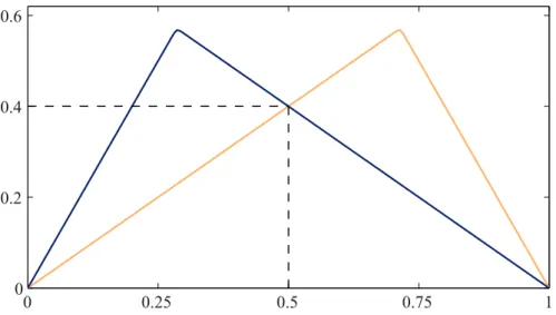
The final results of this section, presented in Table 4, concern a setting, where the tail dependence coefficient stays constant over time whereas the tail copula may change at points (x, y)6= (1,1) (cf. third block of Table 1). From theory, one would expect that the TC-Test should be able to detect those breaks, whereas the TDC-Tests should hold the nominal size. We only consider breaks at ¯s= 0.5 and model (Λ2) (i.e., we simulate from (C2)) which will allow to construct tail copulas that are equal in (1,1), but sufficiently different in other points. More precisely, for a givenλ∈ {0.2,0.4,0.6}, we chooseψ1=λ,ψ2 = 1 andθ= 100 for s≤s¯and we
set ψ1 = 1, ψ2 =λand θ = 100 for s >¯s. For λ= 0.4, the corresponding graphs
of t7→Λ(2−2t,2t) are shown in Figure 1. Note that, for fixed ψ1, ψ2, we have
Λ∞(1−t, t) := lim
θ→∞Λ(1−t, t) ={ψ1(1−t)} ∧(ψ2t).
The corresponding limit copula defined in (10) is the well-known Marshall–Olkin copula, whose TDC is given by min(ψ1, ψ2), see Segers (2012). With our choice of
θ= 100 in (Λ2), the difference between the TDC and min(ψ1, ψ2) =λis less than
the machine accuracy 10−16.
The results in Table 4 confirm the expectations: the TC-Test has considerable power while the TDC-Test 1 basically keeps the nominal size. As a conclusion, the developed testing procedures allow for empirically distinguishing between constant tail dependence coefficient and constant tail copula.
0 0.25 0.5 0.75 1
0 0.2 0.4 0.6
Figure 1: Negative asymmetric logistic model (Λ2) forψ1= 0.4, ψ2 = 1, θ= 100 (blue) andψ1= 1, ψ2= 0.4,θ= 100 (yellow) evaluated on the straight line (2−2t,2t),t∈[0,1]. Both models exhibit the same tail dependence coefficientλ= 0.4.
n = 1 , 000 n = 3 , 000 tail copula Λ(1 , 1) α = 1% α = 5% α = 10% a vg( k ∗) std( k ∗) α = 1% α = 5% α = 10% a vg( k ∗) std( k ∗) i.i.d. setting 0.25 0.0076 0.0460 0.0922 52 23 0.0076 0.0442 0.0934 97 49 (Λ1) 0.50 0.0072 0.0444 0.0924 71 29 0.0088 0.0472 0.0906 134 59 0.75 0.0068 0.0394 0.0846 127 46 0.0082 0.0376 0.0880 237 97 0.20 0.0086 0.0474 0.0946 44 20 0.0090 0.0448 0.0998 80 40 (Λ2) 0.40 0.0100 0.0416 0.0914 61 26 0.0094 0.0466 0.0926 113 52 0.60 0.0066 0.0460 0.0896 84 34 0.0082 0.0452 0.0976 153 67 0.20 0.0098 0.0534 0.1060 47 21 0.0098 0.0558 0.0980 86 44 (Λ1), (Λ2) 0.40 0.0084 0.0444 0.0914 62 26 0.0100 0.0480 0.0922 114 52 0.60 0.0094 0.0466 0.0920 87 33 0.0096 0.0476 0.0930 159 69 AR(1) residual s 0.25 0.0076 0.0462 0.0976 52 23 0.0106 0.0472 0.0992 97 49 (Λ1) 0.50 0.0086 0.0488 0.0906 72 29 0.0110 0.0494 0.0956 134 60 0.75 0.0066 0.0358 0.0812 126 46 0.0084 0.0410 0.0904 235 95 0.20 0.0068 0.0422 0.0926 44 20 0.0088 0.0490 0.0994 81 40 (Λ2) 0.40 0.0074 0.0462 0.0920 61 25 0.0090 0.0452 0.0978 112 42 0.60 0.0088 0.0426 0.0906 83 34 0.0104 0.0454 0.0944 154 67 GAR CH(1,1) residuals 0.25 0.0074 0.0444 0.0908 52 24 0.0084 0.0428 0.0932 99 50 (Λ1) 0.50 0.0068 0.0426 0.0890 72 29 0.0084 0.0468 0.0946 133 59 0.75 0.0060 0.0374 0.0750 124 45 0.0094 0.0424 0.0806 232 93 0.20 0.0080 0.0410 0.0922 44 21 0.0080 0.0418 0.0866 80 41 (Λ2) 0.40 0.0078 0.0426 0.0880 61 26 0.0100 0.0454 0.0908 112 52 0.60 0.0076 0.0404 0.0858 84 33 0.0074 0.0442 0.0936 154 68 T able 1: Sim ulated rejection probabilities of th e TDC-T es t 1 under v arious n ul l h yp oth e ses. In eac h of the residual scenarios, the marginals F and G are standard normally distributed and t -distributed with ν = 3 degrees of freedom, resp ectiv ely . The parameters in the AR(1) setting are set to β1 = 1 / 3 and β2 = 2 / 3.
n = 1 , 000 n = 3 , 000 tail copula Λ(1 , 1) α = 1% α = 5% α = 10% a vg( k ∗ ) std( k ∗ ) α = 1% α = 5% α = 10% a vg( k ∗ ) std( k ∗ ) i.i.d. setting, ¯s = 0 . 5 0.25 to 0.50 0.0512 0.1650 0.2606 61 26 0.1360 0.3090 0.4262 113 53 (Λ1) 0.25 to 0.75 0.3214 0.5632 0.6944 76 30 0.6790 0.8452 0.9042 140 64 0.50 to 0.75 0.0726 0.2112 0.3212 93 35 0.1848 0.3888 0.5072 171 71 0.20 to 0.40 0.0536 0.1754 0.2788 52 22 0.1276 0.3062 0.4306 94 45 (Λ2) 0.20 to 0.60 0.2472 0.4850 0.6132 60 25 0.5466 0.7520 0.8302 111 52 0.40 to 0.60 0.0438 0.1394 0.2312 71 29 0.1048 0.2576 0.3686 130 59 i.i.d. setting, ¯s = 0 . 25 0.25 to 0.50 0.0186 0.0912 0.1740 66 27 0.0536 0.1734 0.2770 122 52 (Λ1) 0.25 to 0.75 0.1250 0.3404 0.4778 95 36 0.3942 0.6496 0.7632 174 74 0.50 to 0.75 0.0356 0.1290 0.2166 107 40 0.0770 0.2248 0.3388 197 82 0.20 to 0.40 0.0218 0.0922 0.1716 56 24 0.0504 0.1606 0.2652 104 49 (Λ2) 0.20 to 0.60 0.0896 0.2622 0.3952 71 29 0.2524 0.4980 0.6396 129 60 0.40 to 0.60 0.0170 0.0792 0.1544 77 31 0.0458 0.1476 0.2384 144 63 AR(1) residuals , ¯s = 0 . 5 0.25 to 0.50 0.0498 0.1636 0.2562 61 26 0.1248 0.2996 0.4202 114 53 (Λ1) 0.25 to 0.75 0.3294 0.5672 0.6898 76 30 0.6860 0.8492 0.9036 138 62 0.50 to 0.75 0.0726 0.2050 0.3106 92 35 0.1902 0.3896 0.5060 169 72 0.20 to 0.40 0.0518 0.1702 0.2616 52 22 0.1328 0.2952 0.4130 96 48 (Λ2) 0.20 to 0.60 0.2562 0.4894 0.6138 61 25 0.5646 0.7656 0.8378 111 53 0.40 to 0.60 0.0444 0.1484 0.2416 71 29 0.1088 0.2676 0.3856 131 59 GAR CH(1,1) residual s, ¯s = 0 . 5 0.25 to 0.50 0.0414 0.1484 0.2464 61 26 0.1388 0.3226 0.4332 112 52 (Λ1) 0.25 to 0.75 0.3174 0.5558 0.6838 76 30 0.6726 0.8416 0.9030 139 61 0.50 to 0.75 0.0694 0.1994 0.2996 91 35 0.1740 0.3728 0.4982 170 72 0.20 to 0.40 0.0560 0.1650 0.2582 52 23 0.1326 0.3062 0.4192 96 47 (Λ2) 0.20 to 0.60 0.2460 0.4736 0.5992 60 25 0.5448 0.7460 0.8306 112 53 0.40 to 0.60 0.0406 0.1376 0.2286 71 29 0.0994 0.2530 0.3614 131 59 T able 2: Sim ulated rejection probabilities of the TDC-T est 1 under v arious alternativ es. In eac h of the residual sc enar ios , the marginals F and G are stand a rd normally distributed and t -distributed with ν = 3 degrees of freedom, resp ectiv ely . The p a ram eters in the AR(1) setting are set to β1 = 1 / 2 and β2 = 1 / 2.
n = 1 , 000 n = 3 , 000 scenario Λ(1 , 1) α = 1% α = 5% α = 10% a vg( k ∗) std( k ∗) α = 1% α = 5% α = 10% a vg( k ∗) std( k ∗) TDC-T est 2, i.i.d. setti n g 0.25 0.005 0.040 0.091 53 24 0.007 0.038 0.097 99 49 H Λ 0 0.50 0.011 0.041 0.088 72 29 0.010 0.046 0.086 134 58 0.75 0.005 0.030 0.068 129 47 0.006 0.046 0.078 236 96 0.25 to 0.50 0.050 0.170 0.260 61 25 0.130 0.300 0.417 115 55 H λ,1 ¯ s = 0 . 5 0.25 to 0.75 0.329 0.563 0.681 77 31 0.711 0.866 0.913 140 61 0.50 to 0.75 0.080 0.225 0.332 93 35 0.194 0.395 0.505 169 71 TC-T est, i.i.d. setting 0.25 0.010 0.070 0.111 52 22 0.011 0.049 0.101 95 46 H Λ 0 0.50 0.009 0.049 0.098 72 29 0.010 0.053 0.099 132 56 0.75 0.008 0.042 0.079 127 46 0.006 0.043 0.082 236 98 0.25 to 0.50 0.047 0.155 0.237 60 24 0.107 0.312 0.427 111 53 H λ,1 ¯ s = 0 . 5 0.25 to 0.75 0.264 0.496 0.616 77 30 0.581 0.774 0.840 135 60 0.50 to 0.75 0.063 0.182 0.277 93 36 0.109 0.271 0.392 170 73 T able 3: Sim ulated rejection probabilities of the TDC-T e st 2 and the TC-T est under the n ull h yp othesis and one alternativ e using the Cla yton copu la within the i.i.d. setting. n = 1 , 000 n = 3 , 000 scenario Λ(1 , 1) α = 1% α = 5% α = 10% a vg( k ∗ ) std( k ∗ ) α = 1% α = 5% α = 10% a vg( k ∗ ) std( k ∗ ) TDC-T est 1, i.i.d. setti n g 0.20 0.009 0.048 0.102 45 21 0.010 0.053 0.103 95 46 H λ 0 ∩ H Λ 1 0.40 0.009 0.049 0.103 63 26 0.009 0.048 0.101 120 53 0.60 0.010 0.053 0.107 89 35 0.012 0.050 0.101 168 72 TC-T est, i.i.d. setting 0.20 0.034 0.163 0.338 46 22 0.242 0.562 0.733 95 46 H λ 0 ∩ H Λ 1 0.40 0.045 0.222 0.421 63 26 0.263 0.634 0.801 121 56 0.60 0.026 0.121 0.301 90 35 0.109 0.480 0.722 168 72 T able 4: Sim ulated rejection prob abilities of the TDC-T es t 1 and the TC-T est: th e first half of the dataset b elongs to mo del (Λ1), the second half to mo del (Λ2). The parameters are chosen suc h that the TDC remains constan t o v er time while the tail copula do es not.
5. Empirical applications
5.1. Energy sector In this section, we reinvestigate the bivariate dataset
from J¨aschke (2012) consisting of n= 1,001 daily closing quotes of WTI Cushing Crude Oil Spot and the Bloomberg European Dated Brent from October 2, 2006, to October 1, 2010, collected from Bloomberg’s Financial Information Services. The analysis of the extremal dependence between the log-returns of the two time series in J¨aschke (2012) is based on the implicit assumption that the tail dependence structure, more precisely their lower tail copula, remains constant over time. We are going to verify this assumption by applying the tests developed in the previous sections.
As pointed out in J¨aschke (2012), the assumption of an i.i.d. sample is unreal-istic. To account for autocorrelation and volatility clustering, it is shown that an ARMA(0,0)-EGARCH(2,3)-model including an explanatory variable (U.S. crude oil inventory) and the skewed generalized error distribution adequately describes the data generating process for the log-returns of the WTI time series. Regarding the daily Brent spot log-returns, an ARMA(1,1)-EGARCH(2,3)-model including U.S. crude oil inventory as an explanatory variable and the skewed generalized error distribution provides an adequate fit.
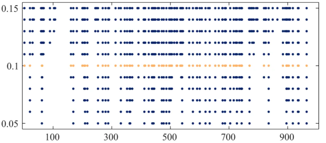
We calculate standardized residuals on the basis of the preceding time series models. A first view on the lower tail dependence between these residuals can be gained from the diagnostic plot in Figure 2. For various values of ksuch that k/n
lies in the set{0.05,0.06, . . . ,0.15}, we depict the points in time where the pseudo-observations in both coordinates fall simultaneously below the valuek/n. Note that these are exactly the joint extremal events inside the indicators in the definition of the empirical tail dependence coefficient. As the points are quite equally spaced in time, the picture suggests that the tail dependence remains rather constant.
100 300 500 700 900
0.05 0.1 0.15
Figure 2: (WTI and Brent time series)Points in time where pseudo-observations in both coordinates fall simultaneously below the valuek/n, fork/n∈ {0.05,0.06, . . . ,0.15}. The yellow row corresponds to the plateau ratiok∗/n= 104/1001≈10%.
More formally, we proceed by checking the hypothesis H0λ of constancy of the tail dependence coefficients by an application of TDC-Test 1. First, in order to obtain a reasonable choice for the parameterk, we use the plateau algorithm from Subsection 3.5 with bandwidth b=b0.005nc = 5. This yields a value of k∗ = 104
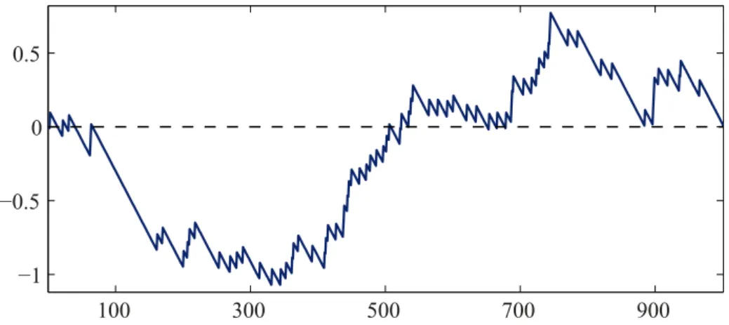
(which is also depicted in yellow in Figure 2) and a plateau of lengthm= 31. Fol-lowing Frahm et al. (2005), the average of the 31 empirical lower tail dependence coefficients on this plateau, given by ˆλ= 0.732, provides a good estimate forλ. Fig-ure 3 shows the corresponding standardized sequential empirical tail copula process
s7→ λˆ−1/2Gn(s,1,1) for k∗ = 104. The graph seems to be indistinguishable from
a simulated path of a one-dimensional standard Brownian bridge, which indicates that the null hypothesis cannot be rejected. In Figure 4, we depict both the value of the the Cram´er-von Mises type test statistic Sn defined in (7) (yellow) as well
as the corresponding p-valuess (blue) as a function of k. The dashed vertical line shows the outcomes for the plateau optimal k∗ = 104, in which case we obtain Sn= 0.285 with a resultingp-value of 0.15. Consequently, the null hypothesis H0λ
cannot be rejected at a 5% level of significance. Moreover, Figure 4 shows that this conclusion is robust with respect to different choices of k. Results for the Kolmogorov-Smirnov-type test and for the TDC-Test 2 are very similar and are not depicted for the sake of brevity.
Finally, the assumption of a constant lower tail copula is verified by testing for the hypothesis H0Λ. We apply the TC-Test from Section 3.2 with B = 2,000 bootstrap replications using the plateau optimal k∗ = 104. We obtain Tn = 0.068 with a resulting p-value of 0.33. Again, the null hypothesis cannot be rejected at a 5% level of significance. Similar as for the tests for H0λ, this conclusion is robust with respect to different choices of k.
100 300 500 700 900 −1
−0.5 0 0.5
Figure 3: (WTI and Brent time series)Standardized sequential empirical tail copula process ˆλ−1/2
Gn(s,1,1) fork∗= 104 with respect tons,s∈[0,1].
5.2. Financial markets As an empirical application from the finance sector,
we consider the Dow Jones Industrial Average and the Nasdaq Composite time series around Black Monday on 19th of October 1987. This dataset coversn= 1,768 log-returns from daily closing quotes between January 4, 1984, and December 31, 1990, collected from Datastream. Related studies in Wied et al. (2013) and Dehling et al. (2013) try to examine whether Black Monday constitutes a break in the dependence structure between the two time series. The outcomes of their studies do not provide a clear picture, as the answer depends on the applied test statistic. While the test for a constant Pearson correlation rejects the null hypothesis of constant correlation, the more robust (rank-based) tests for constant Spearman’s
50 75 100 125 150 0.1
0.3 0.5
Figure 4: (WTI and Brent time series)Test statisticsSn (yellow) and corresponding
p-values (blue) for differentk. The horizontal line indicates the 5% level of significance, the vertical one the plateauk∗= 104.
rho and Kendall’s tau yield no evidence for changes. In these papers, the contrasting result is explained by the fact that the (unfiltered) time series contain several heavy outliers around Black Monday which seriously affect the Pearson-, but not the rank-based tests for Spearman’s rho and Kendall’s tau.
For our analysis, we begin by an investigation of the univariate time series. Applying the model selection and verification criteria from J¨aschke (2012), we find that an ARMA(0,0)-GARCH(1,1)-model witht-distribution for the Dow Jones log-returns and an ARMA(1,0)-GARCH(1,1)-model with skewedt-distribution for the Nasdaq equivalent provide the best fits. Details on the parameter estimation are given in Table 5.
parameter Dow Jones log-returns Nasdaq log-returns estimate std error estimate std error mean equation µ 0.0006 0.0002 0.0005 0.0002 θ1 - - 0.2714 0.0234 variance equation ω 0.0000 0.0000 0.0000 0.0000 α1 0.0349 0.0084 0.1407 0.0179 β1 0.9373 0.0080 0.7914 0.0182 distribution ξ − − 0.8531 0.0294 ν 4.2016 0.4390 5.3001 0.4135
Table 5: Maximum likelihood estimates together with their corresponding standard errors for the Dow Jones ARMA(0,0)-GARCH(1,1)-model with t-distribution and the Nasdaq ARMA(1,0)-GARCH(1,1)-model including the skewedt-distribution. All estimates but the additive constantω are significant at the 1% level.
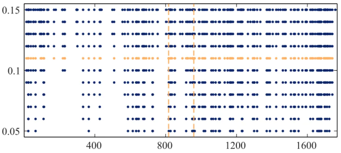
Along the lines of Dehling et al. (2013) we first seek to answer the question whether Black Monday constitutes a break in the tail dependence between the two time series. A positive answer would indicate that the market conditions have substantially changed after this date. For the ease of a clear exposition, we restrict ourselves to an investigation of the lower tail dependence coefficient. A first visual description of the joint tail behavior similar to the one in Figure 2 can be found in Figure 5, which, however, does not provide a clear picture: even though there seems to be a tendency of stronger tail dependence for later dates in the time series, it is unclear whether this is due to a change on Black Monday (second dashed vertical line).
400 800 1200 1600
0.05 0.1 0.15
Figure 5: (Dow Jones and Nasdaq time series) Points in time where pseudo-observations in both coordinates fall simultaneously below the value k/n, for k/n ∈ {0.05,0.06, . . . ,0.15}. The yellow row corresponds to the plateau ratio k∗/n ≈11%. The first yellow vertical line reflects the argmax-estimatorbnsˆλc= 817, the second equivalent indicates Black Mondaybns¯BMc= 959.
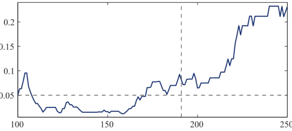
In the following, we examine this formally by applying the tests from Section 3, in particular the test from Section 3.4 for a specific break-point. First, a careful inspection of the plot k 7→ TDC(k) and the statistics defining the plateau algo-rithm (which are not depicted for the sake of brevity) suggests thatk∗ = 191 is a reasonable choice for the parameter k, with a corresponding length of the plateau ofm= 41. The average of the empirical lower tail dependence coefficients over the corresponding values k∈ {171, . . . ,211} is given by ˆλ= 0.620.
Now, we apply the test from Section 3.4 for a specific break-point atbn¯sBMc=
959, the date of Black Monday. The results are depicted in Figure 6, where we plot the p-values of the test against the parameter k. For k∗ = 191, the resulting
p-value of 0.082 does not allow for a clear rejection of the null-hypothesis. In contrast to this, slightly lower values ofkyield to a rejection at the 5%-significance level, whence, as a summary, there seems to be some light, but disputable evidence againstH0. However, the rejection of the null hypothesis might be due to different
reasons than a break precisely on Black Monday. To conclude upon the latter, one would have to accept the hypothesis of constancy of the lower tail dependence coefficient in the subsamples before and after Black Monday. Therefore, we perform the corresponding TDC-Test 1 in the subsamples, whose results are depicted in Figures 7 and 8 in a similar manner as before; in particular, they are based on new
100 150 200 250 0.05
0.1 0.15 0.2
Figure 6: (Dow Jones and Nasdaq time series) Chi-squared test for a break at
bnsBM¯ c = 959: p-values for different k. The horizontal line indicates the 5% level of significance, the vertical one the plateauk∗= 191.
20 40 60 80 100
0 0.05
0.1
Figure 7: (Dow Jones and Nasdaq time series)TDC-Test 1 for the subsample before
bns¯BMc = 959: p-values for different k. The horizontal line indicates the 5% level of significance, the vertical one the plateauk∗= 48.
50 100 150 200 250
0 0.2 0.4 0.6
Figure 8: (Dow Jones and Nasdaq time series)TDC-Test 1 for the subsample after
bns¯BMc = 959 (including Black Monday): p-values for different k. The horizontal line indicates the 5% level of significance, the vertical one the plateauk∗= 169.
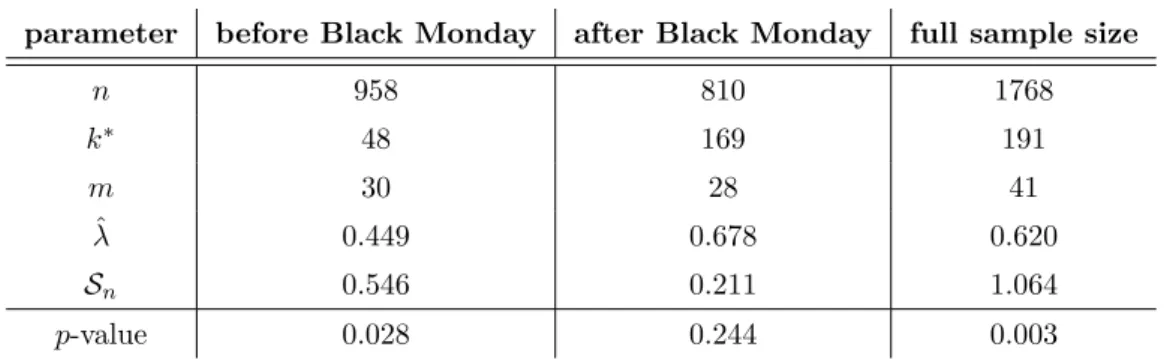
parameter before Black Monday after Black Monday full sample size n 958 810 1768 k∗ 48 169 191 m 30 28 41 ˆ λ 0.449 0.678 0.620 Sn 0.546 0.211 1.064 p-value 0.028 0.244 0.003
Table 6: Summary of results for TDC-Test 1 applied to the subsample before Black Monday, to the subsample after Black Monday and to the full sample.
(plateau-based) choices of k for the reduced samples. We can accept constancy after Black Monday, but have to reject it for the subsample before Black Monday. A summary of the results can also be found in the first two columns of Table 6.
In principal, one could now proceed by a refined analysis of the subsample before Black Monday in order to identify potential additional break-points. Motivated by the diagnostic plot in Figure 5, we prefer an application of the TDC-Test 1 to the whole sample since this might reveal that a model with at most one break-point is also appropriate. In other words, we dismiss the initial guess of a break precisely on Black Monday and rather split the sample at an estimated break-point, hoping that the latter yields to a simpler model with at most one break-point.
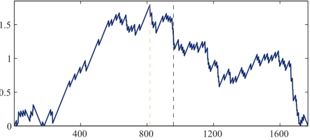
We do not depict the results of the corresponding test, since it clearly rejects the null-hypothesis H0λ at the 1%-significance level for almost all choices of k. A short summary can be found in the last column of Table 6. More enlightening conclusions can be drawn from the plot of the the functionns7→ |λˆ−1/2Gn(s,1,1)|in Figure 9,
fork∗ = 191. The dashed vertical lines denote Black Mondaybns¯BMc= 959 (blue)
and the value bnsˆλc = 817 where the graph attains its maximum (yellow). The latter corresponds to the 27th of March 1987 and appears to be the argmax for most choices of k in a neighborhood of k∗ = 191. We split the sample at this estimated break-point and conduct a refined analysis in the respective subsamples. The procedure is similar to what we have done before, whence we restrict ourselves to a brief summary of the results: in both subsamples, we cannot reject the null hypothesis for all reasonable choices of k, including the values obtained from the plateau algorithm, withp-values lying between 0.2 and 0.5. Similar to the reported values in Table 6 we find ˆλ= 0.430 for the first subsample (k∗= 43) and ˆλ= 0.656 for the second one (k∗ = 57), respectively.
We conclude this application with a short summary of the main findings: (i) The test for a break on Black Monday does not yield entirely unambiguous
results; in particular, we have to reject the null hypothesis of constant tail dependence in the subsample before Black Monday resulting in an overall model with more than one break-point.
(ii) Testing against the existence ofsomeunspecified break-point in the full sample clearly rejects the null, with an estimated break-point atbnsˆλc= 817. Since
we cannot reject the null hypothesis in the corresponding subsamples, an overall model with only one break-point can be accepted.
400 800 1200 1600 0
0.5 1 1.5
Figure 9: (Dow Jones and Nasdaq time series) Absolute standardized sequential empirical tail copula process|λˆ−1/2
Gn(s,1,1)| for k∗ = 191 with respect tons, s∈[0,1].
The yellow vertical line indicates the argmax estimatorbnˆsλc= 817, the black one shows
Black MondaybnsBM¯ c= 959.
6. Conclusion and Outlook
In this paper, we developed new tests for detecting structural breaks in the tail de-pendence of multivariate time series, derived several theoretical properties (asymp-totic null distribution, behavior under alternatives), investigated the finite-sample performance and applied them to datasets from energy and financial markets.
Our work hints at interesting directions for further research. First of all, we did not give a formal proof for the conjecture derived from the simulation study, that the test statistics based on estimated residuals show the same asymptotic behavior as the ones based on i.i.d. samples. To the best of our knowledge, this problem is also unsolved for the estimation techniques described in Section 2: under what conditions does (or does not) the additional estimation step of formingalmost i.i.d. residuals influence the asymptotic behavior of the nonparametric estimators for the tail dependence? Second, extensions to the case of serially dependent datasets (e.g., to mixing sequences) would allow to check for constant tail dependence of the raw data which might also be of interest for practitioners. In particular with a view on the necessary (block) bootstrap procedure this could be a quite challenging task.
A. Appendix
A.1. Proof of the results in the main text For all proofs, by asymptotic
equicontinuity, we may redefine ˆUi = Fn(Xi) and ˆVi = Gn(Yi). For any s ∈[0,1]
and (x, y)∈E, let ˜ Λ◦n(s, x, y) = 1 k bnsc X i=1 1(Ui ≤kx/n, Vi ≤ky/n).
Under H0Λ, this is a sequential (oracle) estimator for Λ◦(s, x, y) = sΛ(x, y). To begin with, we investigate the associated sequential empirical process, defined as
Bn(s, x, y) =
√
The proof of the following lemma is given in Appendix A.2.
Lemma A.1. Suppose that Assumptions 3.1 and 3.2 hold. Then, under H0Λ,
Bn BΛ in (B∞([0,1]×E), d),
where BΛ is given as in Proposition 3.3.
Proof of Proposition 3.3. Since the rank ofXiamongX1, . . . , Xnis the same as the
rank of Ui among U1, . . . , Un (similar for the second coordinate) we may assume
without loss of generality that (Xi, Yi) is distributed according to Ci, i.e., F(x) =
G(x) =xfor all x∈[0,1]. Some thoughts reveal that |Λˆ◦n(s, x, y)−Λ¯◦n(s, x, y)| ≤2/k, uniformly in (s, x, y)∈Sm, where ¯ Λ◦n(s, x, y) = 1 k bnsc X i=1 1 n Xi ≤Fn−(kx/n), Yi≤G−n(ky/n) o
and where Fn− and G−n denote the generalized inverse functions of Fn and Gn,
respectively. Note that ¯Λ◦n can be expressed in terms of ˜Λ◦n as
¯ Λ◦n(s, x, y) = ˜Λ◦n s,n kF − n kx n ,n kG − n ky n .
Now, we have n/kFn(kx/n) = ˜Λ◦n(1, x,∞) and n/kGn(kx/n) = ˜Λ◦n(1,∞, y),
whence, by Hadamard-differentiability of the inverse mapping as stated in B¨ucher and Dette (2011), sup x∈[0,M] n kF − n kx n −x =oP(1), sup y∈[0,M] n kG − n ky n −y =oP(1) (13)
for any M >0 (this result can also be obtained by deducing weak convergence of
x 7→ Bn(1, x,∞) as an element of the c`adl`ag space D([0, M]) with the Skorohod topology (from Lemma A.1), invoking a Skorohod construction and applying Ver-vaat’s Lemma, see Vervaat (1972) or Lemma A.0.2 in de Haan and Ferreira (2006)). Therefore, by asymptotic equicontinuity ofBn,
Gn(s, x, y) = √ k¯ Λ◦n(s, x, y)−sΛ¯◦n(1, x, y) +O(k−1/2) =Bn s,n kF − n kx n ,n kG − n ky n −sBn 1,n kF − n kx n ,n kG − n ky n +O(k−1/2) (14)
weakly converges toGΛ(s, x, y) =BΛ(s, x, y)−sBΛ(1, x, y) on (Sm,k · kSm), for any
m∈N. The Proposition is proved.
Remark A.2. A crucial argument in the preceding proof is the decomposition (14) ofGninto a sum involvingBnfrom Lemma A.1. A similar decomposition is possible