Model-based probabilistic frequent itemset mining

Author(s)

Bernecker, T; Cheng, R; Cheung, DW; Kriegel, HP; Lee, SD;

_{Renz, M; Verhein, F; Wang, L; Zuefle, A}

Citation

Knowledge and Information Systems, 2013, v. 37 n. 1, p. 181-217

Issued Date

2013

URL

http://hdl.handle.net/10722/165826

DOI 10.1007/s10115-012-0561-2

R E G U L A R PA P E R

Model-based probabilistic frequent itemset mining

Hans-Peter Kriegel · Sau Dan Lee · Matthias Renz· Florian Verhein · Liang Wang · Andreas Zuefle

Received: 1 March 2011 / Revised: 30 April 2012 / Accepted: 29 July 2012 © The Author(s) 2012. This article is published with open access at Springerlink.com

Abstract Data uncertainty is inherent in emerging applications such as location-based services, sensor monitoring systems, and data integration. To handle a large amount of impre-cise information, uncertain databases have been recently developed. In this paper, we study how to efficiently discover frequent itemsets from large uncertain databases, interpreted under thePossible World Semantics. This is technically challenging, since an uncertain data-base induces an exponential number of possible worlds. To tackle this problem, we propose a novel methods to capture the itemset mining process as a probability distribution func-tion taking two models into account: the Poisson distribufunc-tion and the normal distribufunc-tion. Thesemodel-based approachesextract frequent itemsets with a high degree of accuracy and

T. Bernecker·H.-P. Kriegel·M. Renz·F. Verhein·A. Zuefle

Department of Computer Science, Ludwig-Maximilians-Universität, Munchen, Germany e-mail: bernecker@dbs.ifi.lmu.de H.-P. Kriegel e-mail: kriegel@dbs.ifi.lmu.de M. Renz e-mail: renz@dbs.ifi.lmu.de F. Verhein e-mail: verhein@dbs.ifi.lmu.de A. Zuefle e-mail: zuefle@dbs.ifi.lmu.de

R. Cheng (

B

Department of Computer Science, University of Hong Kong, Pokfulam, Hong Kong e-mail: ckcheng@cs.hku.hk D. W. Cheung e-mail: dcheung@cs.hku.hk S. D. Lee e-mail: sdlee@cs.hku.hk L. Wang e-mail: lwang@cs.hku.hk

support large databases. We apply our techniques to improve the performance of the algo-rithms for (1) finding itemsets whose frequentness probabilities are larger than some threshold and (2) mining itemsets with thekhighest frequentness probabilities. Our approaches support both tuple and attribute uncertainty models, which are commonly used to represent uncertain databases. Extensive evaluation on real and synthetic datasets shows that our methods are highly accurate and four orders of magnitudes faster than previous approaches. In further theoretical and experimental studies, we give an intuition which model-based approach fits best to different types of data sets.

1 Introduction

In many applications, the underlying databases are uncertain. The locations of users obtained through RFID and GPS systems, for instance, are not precise due to measurement errors [24,

32]. In habitat monitoring systems, data collected from sensors like temperature and humidity are noisy [1]. Customer purchase behaviors, as captured in supermarket basket databases, contain statistical information for predicting what a customer will buy in the future [4,39]. Integration and record linkage tools associate confidence values to the output tuples according to the quality of matching [14]. In structured information extractors, confidence values are appended to rules for extracting patterns from unstructured data [40]. Recently,uncertain databaseshave been proposed to offer a better support for handling imprecise data in these applications [10,14,21,23,30].1

In fact, the mining of uncertain data has recently attracted research attention [4]. For example, in [26], efficient clustering algorithms were developed for uncertain objects; in [22] and [41], naïve Bayes and decision tree classifiers designed for uncertain data were studied. Here, we develop scalable algorithms for finding frequent itemsets (i.e., sets of attribute values that appear together frequently in tuples) for uncertain databases. Our algorithms can be applied to two important uncertainty models:attribute uncertainty(e.g., Table1), and

tuple uncertainty, where every tuple is associated with a probability to indicate whether it exists [13,14,21,30,31].

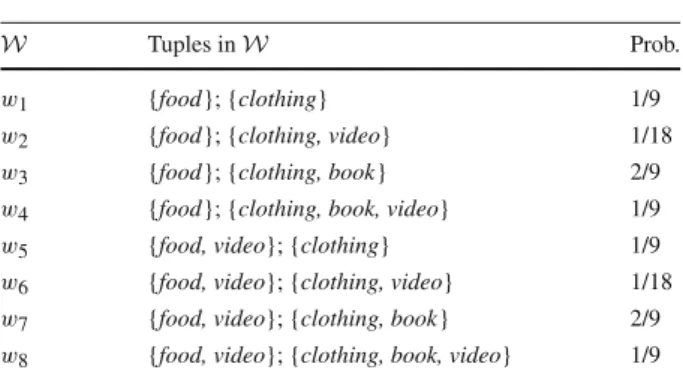
As an example of uncertain data, consider an online marketplace application (Table1). Here, the purchase behavior details of customers Jack and Mary are recorded. The value associated with each item represents the chance that a customer may buy that item in the near future. These probability values may be obtained by analyzing the users’ browsing histories. For instance, if Jack visited the marketplace ten times in the previous week, out of which

videoproducts were clicked five times, the marketplace may conclude that Jack has a 50 % chance of buying, or simply being interested invideos.

To interpret uncertain databases, thePossible World Semantics(or PWS in short) is often used [14]. Conceptually, a database is viewed as a set of deterministic instances (called

possible worlds), each of which contains a set of tuples. Thus, an uncertain transaction databaseD generates a set of possible worldsW. Table2lists all possible worlds for the database depicted in Table1. Each worldwi ∈W, which consists of a subset of attributes from each transaction, occurs with probabilityPr(wi).

For instance, possible world w2 consists of two itemsets, {food} and

{clothing,video}, for Jack and Mary, respectively. The itemset {food} occurs with a proba-bility of1₂, since this itemset corresponds to the set of events that Jack purchases food (prob-ability of one), and Jack does not purchase video (prob(prob-ability of1₂). Assuming independence

Table 1 An uncertain database _{Customer Purchase items}

Jack (video:1/2),(food:1)

Mary (clothing:1),(video:1/3); (book:2/3)

Table 2 Possible worlds of

Table1 W Tuples inW Prob.

w1 {food}; {clothing} 1/9

w2 {food}; {clothing, video} 1/18

w3 {food}; {clothing, book} 2/9

w4 {food}; {clothing, book, video} 1/9

w5 {food, video}; {clothing} 1/9

w6 {food, video}; {clothing, video} 1/18

w7 {food, video}; {clothing, book} 2/9

w8 {food, video}; {clothing, book, video} 1/9

between these events (i.e., the event that Jack buys food does not impact the probability of Jack buying a video game), the joint probability of these events is 1·1₂ = 1₂. Analogously, the probability of obtaining the itemset {clothing,video} for Mary is 1·1₃·1₃ = 1₉. As shown in Table2, the sum of possible world probabilities is one, and the number of possible worlds is exponential in the number of probabilistic items.

Any query evaluation algorithm for an uncertain database has to be correct under PWS. That is, the results produced by the algorithm should be the same as if the query is evaluated on every possible world [14].

Definition 1 (Possible World Semantics (PWS)) Let W be the set of all possible worlds derived from a given uncertain database Dand letϕbe a query predicate. Underpossible world semantics, the probabilityP(ϕ,D)that Dsatisfiesϕis given as the total probability of all worlds that satisfyϕ, that is,

P(ϕ,D)=

w∈W

P(w)·ϕ(w),

whereϕ(w)is an indicator function that returns 1 if worldwsatisfies predicateϕ, and zero otherwise, andP(w)is the probability of worldw.

Our goal is to discover frequent patterns without expandingDinto all possible worlds. Although PWS is intuitive and useful, querying or mining under this notion is costly. This is due to the fact that an uncertain database has an exponential number of possible worlds. For example, the database in Table1has 23 =8 possible worlds. Performing data mining under PWS can thus be technically challenging. On the other hand, ignoring PWS allows to find efficient solutions, for example using expected support only [11]. However, such approaches do not consider probability distributions, that is, are not able to give any probabilistic guarantees. In fact, an itemset whose expected support is greater than a threshold may have a low probability of having a support greater than this threshold. An example of such a scenario can be found in [39].

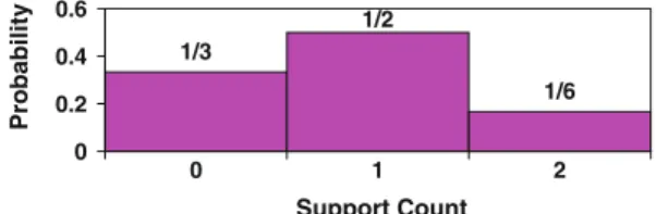
The frequent itemsets discovered from uncertain data are naturally probabilistic, in order to reflect the confidence placed on the mining results. Figure1shows aProbabilistic Frequent

Fig. 1 s-pmf of PFI {video} from Table1 _1/3 1/2 1/6 0 0.2 0.4 0.6 0 1 2 Support Count Probability

Itemset(orPFI) extracted from Table1. APFIis a set of attribute values that occur frequently with sufficiently high probabilities. In Fig.1, thesupport probability mass function(ors-pmf

in short) for thePFI{video} is shown. This is the pmf for the number of tuples (orsupport count) that contain an itemset. Under PWS, a database induces a set of possible worlds, each giving a (different) support count for a given itemset. Hence, the support of a frequent itemset is described by a pmf. In Fig.1, if we consider all possible worlds where itemset {video} occurs twice, the corresponding probability is 1₆.

A simple way of finding PFIs is to mine frequent patterns from every possible world and then record the probabilities of the occurrences of these patterns. This is impractical, due to the exponential number of possible worlds. To remedy this, some algorithms have been recently developed to successfully retrieve PFIs without instantiating all possible worlds [39,46]. These algorithms are able to find a PFI inO(n2)time (wheren is the number of tuples contained in the database). However, our experimental results reveal that they require a long time to complete (e.g., with a 300 k real dataset, the dynamic-programming algorithm in [39] needs 30.1 h to complete).

In this paper, we propose an efficient approximate probabilistic frequent itemset mining solution using specific models to capture the frequentness of an itemset. More precisely, we generalize the model-based approach proposed in [43]. The basic idea is to use appropriate standard parametric distributions to approximate the probabilistic support count, that is, the probability distribution (pmf) of the support count, for both attribute- and tuple-uncertain data. The advantage of such parametric distributions is that they can be computed very efficiently from the transaction database while providing quite good approximation of the support pmf. In particular, this paper introduces a generalized model-based frequent itemset mining approach investigating and discussing three alternatives for modeling the support pmf of itemsets. In addition to the Poisson distribution, which has been used for probabilistic frequent itemset mining and probabilistic ranking [20,43], and the expected support [12], we further investigated the normal distribution for probabilistic frequent itemset mining. Based on these models, we show how the cumulative distribution (cdf) of an itemset associated with the support pmf can be computed very efficiently by means of a single scan of the transaction database. In addition, we provide an in-depth analysis of the proposed models on a theoretical as well as experimental level where we focus on approximation quality and characteristics of the underling data. Here, we evaluate and compare the three models in terms of efficiency, effectiveness, and implementation issues. We show that some of the models are very accurate while some models require certain properties of the data set to be satisfied in order to achieve very high accuracy. An interesting observation is that some models allow us to further reduce the runtime introducing specific pruning criteria, these models, however, lack effectiveness compared to others. We show that the generalizedmodel-based approachruns inO(n)time and is thus more scalable to large datasets. In fact, our algorithm only needs 9.2 s to find all PFIs, which is four orders of magnitudes faster than solutions that are based on the exact support pmf.

In addition, we demonstrate how the model-based algorithm can work under two semantics of PFI, proposed in [39]: (1)threshold-based, where PFIs with probabilities larger than some user-defined threshold are returned; and (2)rank-based, where PFIs with thekhighest probabilities are returned. As we will show, these algorithms can be adapted to the attribute and tuple uncertainty models. For mining threshold-based PFIs, we demonstrate how to reduce the time scanning the database. For mining rank-based PFIs, we optimize the previous algorithm to improve the performance.

We derive the time and space complexities of our approaches. As our experiments show, model-based algorithms can significantly improve the performance of PFI discovery, with a high degree of accuracy. To summarize, our contributions are:

– A generalized model-based approach to approximately compute PFIs efficiently and effectively;

– In-depth study of three s-pmf approximation models based on standard probability mod-els;

– A more efficient method to verify a threshold-based PFI;

– Techniques to enhance the performance of threshold and rank-based PFI discovery algo-rithms, for both attribute and tuple uncertainty models; and

– An extensive experimental evaluation of the proposed methods in terms of efficiency and effectiveness performed on real and synthetic datasets.

This paper is organized as follows. In Sect.2, we review the related work. Section3

discusses the problem definition. Section4describes our model-based support pmf (s-pmf) approximation framework introducing and discussing three models to estimate the s-pmf efficiently and accurately. Then, in Sects.5and6, we present algorithms for discovering threshold- and rank-based PFIs, respectively. Section7presents an in-depth experimental evaluation of the proposed s-pmf approximation models in terms of effectiveness and per-formance results. We conclude in Sect.8.

2 Related work

Mining frequent itemsets is often regarded as an important first step of deriving association rules [5]. Many efficient algorithms have been proposed to retrieve frequent itemsets, such as Apriori [5] and FP-growth [18]. There are also a lot of adaptations for other transaction database settings, like itemset mining in streaming environments [45]; a survey can be found in [28]. While these algorithms work well for databases with precise and exact values, it is interesting to extend them to support uncertain data. Our algorithms are based on the Apriori algorithm. We are convinced that they can be used by other algorithms (e.g., FP-growth) to support uncertain data. In [33], probabilistic models for query selectivity estimation in binary transaction databases have been investigated. In contrast to our work, transactions are assumed to be certain while the probabilistic models are associated with approximate queries on such data.

Solutions for frequent itemset mining in uncertain transaction databases have been inves-tigated in [3,12,42,44]. In [42], an approach for summarizing frequent itemset patterns based on Markov Random Fields has been proposed. In [3,12,44], efficient frequent pattern mining algorithms based on the expected support counts of the patterns have been developed. How-ever, [39,46] found that the use of expected support may render important patterns missing. Hence, they proposed to compute the probability that a pattern is frequent, and introduced the notion of PFI. In [39], dynamic-programming-based solutions were developed to retrieve

Table 3 Our contributions

(marked[√]) Uncertainty Threshold-PFI Rank-PFI

Attribute Exact [39] Exact [39]

Approx.[√] Approx.[√]

Tuple Exact [38]

Approx. (singleton) [46] Approx.[√] Approx. (multiple items)[√]

PFIs from attribute-uncertain databases, for both threshold- and rank-based PFIs. However, their algorithms have to compute exact probabilities and compute a PFI inO(n2)time. By using probability models, our algorithms avoid the use of dynamic programming, and can find a PFI much faster (inO(n)time). In [46], approximate algorithms for deriving threshold-based PFIs from tuple-uncertain data streams were developed. While [46] only considered the extraction of singletons (i.e., sets of single items), our solution discovers patterns with more than one item. More recently, [38] developed an exact threshold-based PFI mining algorithm. However, it does not support rank-based PFI discovery. Here, we also study the retrieval of rank-based PFIs from tuple-uncertain data. To the best of our knowledge, this has not been examined before. Table3summarizes the major work done in PFI mining.

Other works on the retrieval of frequent patterns from imprecise data include: [9], which studied approximate frequent patterns on noisy data; [27], which examined association rules on fuzzy sets; and [29], which proposed the notion of a “vague association rule”. However, none of these solutions are developed on the uncertainty models studied here.

3 Problem definition

In Sect.3.1, we discuss the uncertainty models used in this paper. Then, we describe the notions of threshold- and rank-based PFIs in Sect.3.2.

3.1 Attribute and tuple uncertainty

LetVbe a set of items. In theattribute uncertainty model[10,23,32,39], each attribute value carries some uncertain information. Here, we adopt the following variant [39]: a database

D containsntuples, or transactions. Each transactiontj is associated with a set of items taken fromV. Each itemv ∈ V exists intj with an existential probability Pr(v ∈tj) ∈ (0,1], which denotes the chance thatvbelongs totj. In Table1, for instance, the existential probability ofvideointJ ackisPr(vi deoJ ack)=1/2. This model can also be used to describe uncertainty in binary attributes. For instance, the itemvi deocan be considered as an attribute, whose value is one, for Jack’s tuple, with probability1₂, in tupletJ ack.

Under the possible world semantics (PWS), D generates a set of possible worldsW. Table2lists all possible worlds for Table1. Each worldwi ∈W, which consists of a subset of attributes from each transaction, occurs with probabilityPr(wi). For example,Pr(w2)is

the product of: (1) the probability that Jack purchasesfoodbut notvideo(equal to1₂) and (2) the probability that Mary buysclothingandvideoonly (equal to1₉). As shown in Table2, the sum of possible world probabilities is one, and the number of possible worlds is exponentially large. Our goal is to discover frequent patterns without expandingDinto possible worlds.

In thetuple uncertainty model, each tuple or transaction is associated with a probability value. We assume the following variant [13,31]: each transactiontj ∈Dis associated with a

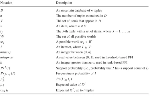
Table 4 Summary of notations

Notation Description

D An uncertain database ofntuples

n The number of tuples contained inD

V The set of items that appear inD

v An item, wherev∈V

tj Thej-th tuple with a set of items, wherej=1, . . . ,n

W The set of all possible worlds

wj A possible worldwj∈W

I An itemset, whereI⊆V

mi nsup An integer between(0,n]

mi npr ob A real value between(0,1], used in threshold-based PFI

k An integer greater than zero, used in rank-based PFI

PrI(i) Support probability (i.e., probability thatIhas a support count ofi) Prf r eq(I) Frequentness probability ofI

pI_j Pr(I⊆tj)

μI Expected value ofXI

(μI)l ExpectedXI, up toltuples

set of items and an existential probabilityPr(tj)∈(0,1], which indicates thattjexists inD with probabilityPr(tj). Again, the number of possible worlds for this model is exponentially large. Table4summarizes the symbols used in this paper.

3.2 Probabilistic frequent itemsets (PFI)

LetI ⊆Vbe a set of items, or anitemset. ThesupportofI, denoted bys(I), is the number of transactions in whichI appears in a transaction database [5]. In precise databases,s(I)

is a single value. This is no longer true in uncertain databases, because in different possible worlds,s(I)can have different values. LetS(wj,I)be the support count ofI in possible worldwj. Then, the probability thats(I)has a value ofi, denoted by PrI(i), is:

PrI(i)=

wj∈W,S(wj,I)=i

Pr(wj) (1)

Hence,PrI(i)(i=1, . . . ,n)form aprobability mass function(orpmf) ofs(I). We callPrI

thesupport pmf(ors-pmf) ofI. In Table2, for instance,Pr{video}(2)=Pr(w6)+Pr(w8)= 1

6, sinces(I)=2 in possible worldsw6andw8. Figure1shows the s-pmf of {video}.

Now, letmi nsup ∈ (0,n]be an integer. An itemset I is said to befrequentifs(I) ≥ mi nsup[5]. For uncertain databases, thefrequentness probabilityofI, denoted byPrf r eq(I), is the probability that an itemset is frequent [39]. Notice thatPrf r eq(I)can be expressed as:

Prf r eq(I)= i≥mi nsup

PrI(i) (2)

Using frequentness probabilities, we can determine whether an itemset is frequent. We identify two classes ofProbabilistic Frequent Itemsets(orPFI) below:

– I is athreshold-based PFI if its frequentness probability is larger than some thresh-old [39]. Formally, given a real valueminprob ∈(0,1],I is a threshold-based PFI, if

Prf r eq(I)≥minprob. We callminprobthefrequentness probability threshold. – Iis arank-based PFIif its frequentness probability satisfies some ranking criteria. The

top-kPFI, proposed in [39], belongs to this class. Given an integerk >0,Iis a top-k

PFI ifPrf r eq(I)is at least thek-th highest, among all itemsets. We focus on top-kPFI in this paper.

Before we move on, we would like to mention the following theorem, which was discussed in [39]:

Theorem 1 Anti-Monotonicity: Let S and I be two itemsets. If S⊆I, then Prf r eq(S)≥

Prf r eq(I).

This theorem will be used in our algorithms.

Next, we derive efficient s-pmf computation methods in Sect.4. Based on these methods, we present algorithms for retrieving threshold-based and rank-based PFIs in Sects.5and 6, respectively.

4 Approximation of S-pmf

From the last section, we can see that the s-pmfs(I)of itemsetI plays an important role in determining whetherIis a PFI. However, directly computings(I)(e.g., using the dynamic programming approaches of [39,46]) can be expensive. We now investigate alternative ways of computings(I). In the following, we study some statistical properties ofs(I)and show how to approximate the distribution ofs(I)in a computationally efficient way by means of the expected support (cf. Sect.4.1) and two standard probability distributions: the Poisson distribution (cf. Sect.4.2) and the normal distribution (cf. Sect.4.3). In Sect.4.4, we discuss all three alternatives.

An interesting observation abouts(I) is that it is essentially the number of successful

Poisson trials[37]. To explain, we letXI_j be a random variable, which is equal to one ifIis a subset of the items associated with transactiontj (i.e.,I ⊆tj), or zero otherwise. Notice thatPr(I⊆tj)can be easily calculated in our uncertainty models:

– Forattribute uncertainty,

Pr(I⊆tj)=

v∈I

Pr(v∈tj) (3)

– Fortuple uncertainty,

Pr(I ⊆tj)=

Pr(tj) ifI⊆tj

0 otherwise (4)

Given a database of sizen, eachIis associated with random variablesX₁I,X₂I, . . . ,X_nI. In both uncertainty models considered in this paper, all tuples are independent. Therefore, these

nvariables are independent, and they representnPoisson trials. Moreover,XI=n_j=1XI_j

Next, we observe an important relationship betweenXIandPrI(i)(i.e., the probability that the support ofIisi):

PrI(i)=Pr(XI =i) (5) This is simply becauseXI is the number of times thatI exists in the database. Hence, the s-pmf ofI, that is,PrI(i), is the pmf ofXI, a Poisson binomial distribution.

Using Eq.5, we can rewrite Eq.2, which computes the frequentness probability ofI, as:

Prf r eq(I)= i≥mi nsup

PrI(i) (6)

=1−Pr(XI ≤minsup−1) (7) LetPr_≤I(i)be the cumulative distribution function (cdf) ofXI, that is,

Pr_≤I(i)=

j=0..i

PrI(j). (8)

Therefore, if the cumulative distribution function Pr_≤I(i)of XI is known, Prf r eq(I)can also be evaluated efficiently:

Prf r eq(I)=1− i≤mi nsup−1

PrI(i) (9)

=1−Pr_≤I(mi nsup−1). (10) Next, we discuss approaches to approximate this cdf, in order to compute Prf r eq(I) efficiently.

4.1 Approximation by expected support

A simple and efficient way to evaluate the frequentness of an itemset in an uncertain trans-action database is to use the expected support [3,12]. The expected support converges to the exact support when increasing the number of transactions according to the “law of large numbers.”

Definition 2 (Law of Large Numbers) A “law of large numbers” is one of several theorems expressing the idea that as the number of trials of a random process increases, the percentage difference between the expected and actual values goes to zero. Formally, given a sequence of independent and identically distributed random variablesX1, . . . ,Xn, the sample average

1

n

n

i=1Xi converges to the expected value μ =

n

i=1E(Xi) forn → ∞. It can also be shown ([17]), that the law of large numbers is applicable for non-identically distributed random variables.

For notational convenience, letpI_j be Pr(I ⊆tj). Since the expectation of a sum is the sum of the expectations, the expected value ofXI, denoted byμI, can be computed by:

μI = n

j=1

pI_j (11)

Given the expected supportμI, we can approximate the cdfPr_≤I(i)ofXI as follows:

Pr_≤I(i)=

0 ifi < μI

0 1 2 3 0.0 0 .2 0.4 0.6 0.8 1.0 Support Probability Exact Expected 0 1 2 3 0.0 0 .2 0.4 0.6 0.8 1.0 Support Probability Exact Poisson

(a) Expected approximation (b) Poisson approximation

Fig. 2 Approximations of the s-pmf of PFI {video} from Table1

According to the above equation, the frequentness probability Prf r eq(I) of itemset I is approximated by 1, ifμI is at leastmi nsupand 0 otherwise. The computation ofμI can be efficiently done by scanningDonce and summing uppI_j’s for all tuplestj inD. As an example, consider the support of itemset{vi deo}in Table1. ComputingμI =0.5+0.33 yields the approximated pmf depicted in Fig.2a. Obviously, the expected support is only a very coarse approximation of the exact support distribution. Important information about the distribution, for example the variance, is lost with this approximation. In fact, we do not know how confident the results are. In the following, we provide a more accurate approximation forPr_≤I(i)by taking the (exact) distribution into consideration.

4.2 Poisson Distribution-Based Approximation

A Poisson binomial distribution can be well approximated by a Poisson distribution [8] following the “Poisson law of small numbers”.

Definition 3 (Poisson Law of Small Numbers) Given a sequence of independent ran-dom Bernoulli variables X1, . . . ,Xn, with mean (μ)i, the density of the sample aver-age X = _n1n_i=1Xi is approximately Poisson distributed with λX = 1_n

n

i=1(μ)i if max{P(X1), . . . ,P(Xn)}tends to zero [19].

According to this law, Eq.10can be written as:

Prf r eq(I)≈1−Fp(minsup−1, μI) (13) whereFpis the cdf of the Poisson distribution with meanμI, that is,Fp(minsup−1, μI)= 1−Γ (minsup,μI)

(minsup−1)! , whereΓ (minsup, μI)=

_∞

μI t

minsup−1_e−t_dt.

As an example, consider again the support of itemset{vi deo}in Table 1. Computing

μ=λI _{=0.5+0.33 yields the approximated pmf depicted in Fig.2b. A theoretical analysis} of the approximation quality is shown in Appendix8. The upper bound of the error is small. According to our experimental results, the approximation is quite accurate.

To estimatePrf r eq(I), we can first computeμIby scanningDonce as described above and evaluateFp(minsup−1, μI). Then, Eq.13is used to approximatePrf r eq(I).

0 1 2 3 0.0 0 .2 0.4 0.6 0.8 1.0 Support Probability _Exact Normal 0 1 2 3 0.0 0 .2 0.4 0.6 0.8 1.0 Support Probability Exact Normal+

(a)Normal distribution-based approximation (b)Approximation with continuity correction

Fig. 3 Itemset support distribution approximated with the normal distribution.aNormal distribution-based approximation.bApproximation with continuity correction

4.3 Normal Distribution-Based Approximation

Provided|D|is large enough which usually holds for transaction databases,XIconverges to the normal distribution with meanμIand varianceσI2, where

σ2 I =V ar(XI)= tj∈D Pr(I ⊆tj)·(1−Pr(I⊆tj))= n j=1 pI_j · 1−pI_j

according to the “Central Limit Theorem”.

Definition 4 (Central Limit Theorem) Given a sequence of independent random vari-ables X1, . . . ,Xn, with meanμi and finite varianceσi2, the density of the sample aver-age X = 1_nn_i=1Xi is approximately normal distributed with μX = 1_n

n

i=1μi and σ2

X =√1_nni=1σ2i.

Lemma 1 The support probability distribution of an itemset I is approximated by the normal distribution with meanμIand varianceσI2as defined above. Therefore,

Prf r eq(I)≈1−Fn(minsup−1, μI, σI2) (14)

where Fn is the cdf of the normal distribution with meanμIand varianceσ_I2, that is,

Fn(minsup−1, μI, σI2)= 1 σI √ 2π mi nsup−0.5 −∞ e− (x−μI)2 2σ2 I ₍₁₅₎

Computingμ= 0.5+0.33 andsigma2 _{= 0.5·0.5+0.33·0.67= 0.471 yields the}

approximated pmf depicted in Fig.3a. The continuity correction which is achieved by running the integral up tomi nsup−0.5 instead ofmi nsup−1 is an important and common method to compensate the fact thatXIis a discrete distribution approximated by a continuous normal distribution. The effect of the continuity correction is shown in Fig.3b.

The estimation of Prf r eq(I)can be done by first computingμI by scanningD once, summing uppI_j’s for all tuplestjinDand using Eq.14to approximatePrf r eq(I). For an efficient evaluation ofFn(minsup−1, μI), we use the Abromowitz and Stegun approxima-tion [2] which is necessary because the cumulative normal distribution has no closed-form solution. The result is a very fast parametric test to evaluate the frequentness of an itemset.

While the above method still requires a full scan of the database to evaluate one frequent itemset candidate, threshold- and rank-based PFIs can be found more efficiently.

4.4 Discussion

In this section, we have described three models to approximate the Poisson binomial distri-bution. Now, we will discuss the advantages and disadvantages of each model theoretically, while in Sect.7we will experimentally support the claims made here.

Each of the approximation models is based on a fundamental statistics theorem. In particular, theExpectedapproach exploits theLaw of Large Numbers[35], theNormal Approximationapproach exploits theCentral Limit Theorem[16], and thePoisson Approxi-mationapproach exploits thePoisson Law of Small Numbers[34].

Approximation based on expected supportIn consideration of the “Law of large numbers,” theExpectedapproach requires a largen, that is, a large number of transactions, where the respective itemset is contained with a probability greater than zero. A thorough evaluation of this parameter can be found in the experiments.

Normal distribution-based approximationThe rule of thumb for the central limit theorem is, is that forn ≥30, that is, for at least 30 transactions containing the respective itemset with a probability larger than zero, the normal approximation yields good results. This rule of thumb, however, depends on certain circumstances, namely, the probabilitiesP(Xi =1) should be close to 0.5. In our experiments, we will evaluate for what settings (e.g., databases size, itemset probabilities) the normal approximation yields good results.

Poisson distribution-based approximationIn consideration of thePoisson Law of Small Numbers, the Poisson approximation theoretically yields good results, ifall probabilities

P(Xi)are small. This seems to be a harsh assumption, since it forbids any probabilities of one, which are common in real data sets. However, it can be argued that, for large itemsets, the probability may always become small in some applications. In the experiments, we will show how small max{P(X1), . . . ,P(Xn)}is required to be, in order to achieve good approximations, and how “a few” large probabilities impact the approximation quality. In addition, our experiments aim to give an intuition, in what setting which approximation should be used to achieve the best approximation results.

Computational complexity Each approximation technique requires to compute the expected supportE(X)=μ=λ=n_i=1P(Xi), which requires a full scan of the database requiring O(n) time andO(1)space. The normal approximation additionally requires to compute the sum of variances, which has the same complexity. This is all that has to be done to compute the parameters of all three approximations. After that, the Expected approach only requires to compareE(X)withMi n Supp, at a cost ofO(1)time. The normal approximation approach in contrast requires to compute the probability thatX>Mi n Supp, which requires numeric integration, since the normal distribution it has no closed-form expression. However, there exist very efficient techniques (such as the Abromowitz and Stegun approximation [2]) to quickly evaluate the normal distribution. Regardless, this evaluation is independent of the database size and also requires constant time. The same rationale applies for the Poisson approximation, which does also not have a closed-form solution, but for which there exist

manifold fast approximation techniques. In summary, each of the approximation techniques has a total runtime complexity ofO(n+Ci)and a space complexity ofO(1). The constant

Cidepends on the approximation technique. In the experiments, we will see that the impact ofCi can be neglected in runtime experiments. In summary, each of the proposed approxi-mation techniques runs in O(n) time. These are more scalable methods compared to solutions in [39,46], which evaluatePrf r eq(I)inO(n2)time.

5 Threshold-based PFI mining

Can we quickly determine whether an itemsetI is a threshold-based PFI? Answering this question is crucial, since in typical PFI mining algorithms (e.g., [39]), candidate itemsets are first generated, before they are tested on whether they are PFI’s. In Sect.5.1, we develop a simple method of testing whetherIis a threshold-based PFI, without computing its frequent-ness probability. This method is applicable for any s-pmf approximation proposed in Sect.4. We then enhance this method in Sect.5.2by adding pruning techniques that allow to decide whether an itemset must (not) be frequent based on a subset of the database only. Finally, we demonstrate an adaptation of these techniques in an existing PFI mining algorithm, in Sect.5.3.

5.1 PFI Testing

Given the values ofmi nsupandmi npr ob, we need to test whether Iis a threshold-based PFI. Therefore, we first need the following definition:

Definition 5 (p-value) LetXbe a random variable with pmf pm fXon the domainR. The

p-valueof X at x denotes the probability that X takes a value less than or equal tox. Formally,

p-value(x,X)=

x

−∞

pm fX(x).

Given the cumulative mass functioncm fXofX, this translates into

p-value(x,X)=cm fX(x)

The computation of the p-value is an inherent method in any statistical program package. For instance, in the statistical computing packageR, the p-value of a valuex of a normal distribution with meanμand varianceσ2is obtained using the functionpnor m(x, μ, σ2). For the Poisson distribution, the function ppoi s(x, μ)is used. For the expected approximation, simply return 1 isμ >mi nsupand 0 otherwise.

Sincep-value(mi nsup,suppor t(I))corresponds to the probability that the support of itemset I is equal or less than mi nsup, we can derive the probability Prf r eq(I)that the support is at leastmi nsupsimply as follows:

Prf r eq(I)=1−(p-value(mi nsup,suppor t(I))+P(suppor t(I)=mi nsup)) which is approximated by

whereP(suppor t(I)=mi nsup)is the probability that the support ofI is exactly minsup, andis a very small number (e.g.,=10{−10}_).

Now, to decide whether I is a threshold-based PFI, given the values ofmi nsup and

mi npr obwe apply the following three steps:

– Compute the parametersμI(andσ_I2for the normal case).

– Derive the probability Prf r eq(I) = 1−(p-value(mi nsup−,suppor t(I)) given

mi nsupand the respective approximation model support(I).

– ifPrf r eq(I) > mi npr ob, returnI as a frequent itemset, otherwise, conclude thatI is not a frequent itemset.

Example 1 Consider again the example given in Table1. Assume that we want to decide whether itemset{vi deo}has a support of at leastmi nsup=1 with a probability of at least 60 %. Assume that we want to use the normal approximation model. Therefore, in the first step, we compute the approximation parametersμ_{vi deo}=0.5+0.33=0.83 andσ_{v2_{i deo}}= 0.5·0.5+0.33·0.67=0.47. Next, we computep-value(mi nsup,suppor t({vi deo})), which corresponds to evaluating the dotted cdf in Fig.3atmi nsup=1, which yields a probability of about 90 %. Since this value is greater thanmi npr ob=60%, we are able to conclude that itemset{vi deo}must be frequent formi nsup=1 andmi npr ob=60%.

In the following, we show pruning techniques which are applicable for the expected support model as well as the Poisson approximation model. For the normal approximation, we give a counter-example, why the proposed pruning strategy may yield wrong results. 5.2 Improving the PFI testing process for the poisson approximation

In Step 1 of the last section,Dhas to be scanned once to obtainμIandσI2, for every itemsetI. This can be costly ifDis large, and if many itemsets need to be tested. For example, in the Apriori algorithm [39], many candidate itemsets are generated first before testing whether they are PFIs. In the following, we will define a monotonicity criterion which can be used to decide ifIis frequent by only scanning a subset of the database. In the following, we will show that for the model using expected support and for the Poisson approximation model, the above lemma holds, that is,(Prf r eq(I))i increases monotonically ini. For the normal approximation, however, we will show a counter-example to illustrate that the above property does not hold.

Definition 6 (n-Monotonicity) Leti∈(0,n]. Let(XI)i be an approximation model of the support of itemsetI, based on the firsti transactions, that is, on the parameters(μI)i and (σ2

I)i. Also, let(Prf r eq(I))i denote the probability thatIhas a support of at least minsup, given these parameters. If(Prf r eq(I))i ≥mi npr ob, thenIis a threshold-based PFI.

Lemma 2 Property6holds for the approximation model using the expected support.

Proof Let(XI)i denote the approximation of the smf of itemsetIusing expected support. Therefore,(Prf r eq(I))iequals to 1, if(μI)i>mi nsupand to 0 otherwise. Now consider the

probability(Prf r eq(I))i+1. Trivially, if(Prf r eq(I))i=0, then it holds that(Prf r eq(I))i< (Prf r eq(I))i+1. Otherwise, it holds that (Prf r eq(I))i = 1 which implies that (μI)i >

mi nsup. Since

(μI)j =(μI)i+pj≥(μI)i>mi nsup it holds that(Prf r eq(I))i+1=1.

Thus in all casesp-value(mi nsup, (XI)i)is non decreasing ini.

Lemma 3 Property6holds for the Poisson approximation model.

Proof In the previous proof, we have exploited that(μI)iincreases monotonically ini. To show that(Prf r eq(I))i increases monotonically iniif the Poisson approximation is used,

we only have to show the following

Theorem 2 Prf r eq(I), if approximated by Eq.13, increases monotonically withμI. The cdf of a Poisson distribution,Fp(i, μ), can be written as: Fp(i, μ) = Γ (i+_i!1,μ) =

∞

μ t(i+1)−1e−tdt i!

Sincemi nsupis fixed and independent ofμ, let us examine the partial derivative w.r.t.μ.

∂Fp(i, μ) ∂μ = ∂ ∂μ _∞ μ t(i+1)−1e−tdt i! = 1 i! ∂ ∂μ ⎛ ⎝ ∞ μ tie−tdt ⎞ ⎠ = 1 i!(−μie −μ₎ = −fp(i, μ)≤0

Thus, the cdf of the Poisson distributionFp(i, μ)is monotonically decreasing w.r.t.μ, wheniis fixed. Consequently, 1−Fp(i−1, μ)increases monotonically withμ. Theorem2 follows immediately by substitutingi=minsup.

Note that intuitively, Theorem2states that the higher value ofμI, the higher is the chance thatIis a PFI.

Lemma 4 Property6does not hold for the normal approximation model.

Proof For the normal approximation, we give a counter-example, which illustrates that

Prop-erty6does not hold.

Example 2 Assume that itemsetI is contained in transactionst1 andt2 with probabilities

of 1 and 0.5, respectively. Assume thatmi nsup =1. Since p1 = P(I ∈t1) =1, we get (μI)1=1 and(σI2)1=1·0=0. Computing(Prf r eq(I))1yields 1, since the normal pmf

with parametersμ=1 andσ2 _{=0 is 1 with a probability of 1 and thus is always greater}

or equal thanmi nsup=1. Now, consider(Prf r eq(I))2: To evaluate this, we use a normal

distribution with parameters(μI)2 =1+0.5=1.5 and(σ_I2)2=1·0=0+0.5·0.5=0.25.

Since the normal pmf is unbounded forσ2 = 0, it is clear that(Prf r eq(I))2 < 1, since

Property6leads to the following:

Lemma 5 Let i ∈(0,n]and assume that(Prf r eq(I))i is approximated using the expected

support model or using Poisson approximation. Then, it holds that if (Prf r eq(I))i >

mi npr ob then Prf r eq(I) >mi npr ob and I can be returned as an approximate result.

Proof Notice that(μI)imonotonically increases withi. If there exists a value ofisuch that (μI)i≥(μ)m, we must haveμI =(μI)n≥(μI)i≥(μ)m, implying thatI is a PFI.

Using Lemma5, a PFI can be verified by scanning only a part of the database.

True hitsLet(μI)l = lj=1pj and(σ_I2)l = lj=1pj ·(1− pj), wherel ∈ (0,n]. Essentially,(μI)l((σI2)l) is the “partial value” ofμI(σI2), which is obtained after scanning

ltuples. Notice that(μI)n =μIand(σI2)n=σI2.

To perform pruning based on the values of(μI)land(σI2)l, we first define the following property:

Avoiding integrationWe next show the following. To perform the true hit detection as proposed above, we require to evaluate(Prf r eq(I))ifor eachi ∈1, . . . ,n. In the case of the expected support approximation, this only requires to check if(μI)i >mi nsup. However, for the Poisson approximation, this requires to evaluate a poisson distribution at minsup. Since the Poisson distribution has no closed-form solution, this requires a large number of numeric integrations, which can be, depending on their accuracy, computationally very expensive. In the following, we show how to perform pruning using the Poisson approximation model, while avoiding the integrations.2

Given the values ofmi nsupandmi npr ob, we can test whether(Prf r eq(I))i>mi npr ob as follows:

Step 1.Find a real number(μ)msatisfying the equation:

mi npr ob=1−Fp/n(mi nsup−1, (μ)m), (16) whereFp/ndenotes the cdf of the Poisson distribution. The above equation can be solved efficiently by employing numerical methods, thanks to Theorem2. This computation has to be performed only once.

Step 2.Use Eq.11to compute(μI)i.

Step 3.If(μI)i≥(μ)m, we conclude thatIis a PFI. Otherwise,I must not be a PFI. To understand why this works, first notice that the right side of Eq.16is the same as that of Eqs.13or14, an expression of frequentness probability. Essentially, Step 1 finds out the value of(μ)m that corresponds to the frequentness probability threshold (i.e.,minprob). In Steps 2 and 3, ifμI ≥(μ)m, Theorem2allows us to deduce thatPrf r eq(I) > minprob. Hence, these steps together can test whether an itemset is a PFI.

In order to verify whetherI is a PFI, once(μ)m is found, we do not have to evaluate (Prf r eq(I))i. Instead, we compute(μI)iin Step 2, which can be done in O(1)time using (μI)i−1. In the next paragraph, we show how the observation made in this paragraph can be

used to efficiently detect true drops, that is, itemsets for which we can decide thatμI < (μ)m by only considering(μI)i.

2_{Recall that true hit detection is not applicable for normal approximation, which is the reason why normal}

True Drops

Lemma 6 If I is a threshold-based PFI, then:

(muI)n−i ≥(μ)m−i∀i∈(0,(μ)m] (17)

Proof LetDlbe a set of tuples{t1, . . . ,tl}. Then, μI= n j=1 Pr(I⊆tj);(μI)i= i j=1 Pr(I⊆tj) SincePr(I⊆tj)∈ [0,1], based on the above equations, we have:

i≥μI−(μI)n−i (18) If itemsetI is a PFI, thenμI ≥(μ)m. In addition,(μI)n−i≥0. Therefore,

i ≥μI−(μI)n−i ≥(μ)m−(μI)n−i f or0<i≤ (μ)m

⇒ (μI)n−i ≥(μ)m−ifor 0<i ≤ (μ)m

This lemma leads to the following corollary.

Corollary 1 An itemset I cannot be a PFI if there exists i∈(0,(μ)m]such that:

(μI)n−i < (μ)m−i (19)

We use an example to illustrate Corollary1. Suppose that(μ)m=1.1 for the database in Table1. Also, letI= {clothing, video}. Using Corollary1, we do not have to scan the whole database. Instead, only the tupletJ ackneeds to be read. This is because:

(μI)1=0<1.1−1=0.1 (20)

Since Eq.19is satisfied, we confirm thatIis not a PFI without scanning the whole database. We use the above results to improve the speed of the PFI testing process. Specifically, after a tuple has been scanned, we check whether Lemma5is satisfied; if so, we immediately conclude thatIis a PFI. After scanningn− (μ)mor more tuples, we examine whetherIis not a PFI, by using Corollary1. These testing procedures continue until the whole database is scanned, yieldingμI. Then, we execute Step 3 (Sect.5.1) to test whetherIis a PFI. 5.3 Case study: the Apriori algorithm

The testing techniques just mentioned are not associated with any specific threshold-based PFI mining algorithms. Moreover, these methods support both attribute and tuple uncertainty models. Hence, they can be easily adopted by existing algorithms. We now explain how to incorporate our techniques to enhance the Apriori [39] algorithm, an important PFI mining algorithms.

The resulting procedures (Algorithm 1 for Poisson approximation and expected support, and Algorithm 2 for normal approximation) use the “bottom-up” framework of the Apriori: starting fromk=1, size-kPFIs (calledk-PFIs) are first generated. Then, using Theorem1, size-(k+1)candidate itemsets are derived from thek-PFIs, based on which thek-PFIs are found. The process goes on with largerk, until no larger candidate itemsets can be discovered.

The main difference of Algorithm 1 and Algorithm 2 compared with that of Apriori [39] is that all steps that require frequentness probability computation are replaced by our PFI testing methods. In particular, Algorithm 1 first computes(μ)m (Line 2–3) depending on whether the expected support model or the Poisson approximation model is used.

Then, for each candidate itemset I generated on Line 4 and Line 17, we scan D and compute its(μI)i (Line 10) and(σI2)i. Unless the normal approximation is used, pruning can now be performed: If Lemma5is satisfied, then I is put to the result (Lines 11–13). However, if Corollary1is satisfied,Iis pruned from the candidate itemsets (Lines 14–16). This process goes on until no more candidates itemsets are found.

Complexity.In Algorithm 1, each candidate item needsO(n)time to test whether it is a PFI. This is much faster than the Apriori [39], which verifies a PFI inO(n2)time. Moreover, sinceDis scanned once for allk-PFI candidatesCk, at most a total ofntuples is retrieved for eachCk(instead of|Ck| ·n). The space complexity isO(|Ck|)for each candidate setCk, in order to maintainμI for each candidate.

6 Rank-based PFI mining

Besides mining threshold-based PFIs, the s-pmf approximation methods presented in Sec-tion4can also facilitate the discovery of rank-based PFIs (i.e., PFIs returned based on their relative rankings). In this section, we investigate an adaptation of our methods for finding top-k PFIs, a kind of rank-based PFIs which orders PFIs according to their frequentness probabilities.

Our solution (Algorithm 3) follows the framework in [39]: A bounded priority queue,

Q, is maintained to store candidate itemsets that can be top-kPFIs, in descending order of their frequentness probabilities. Initially,Q has a capacity ofkitemsets, and single items with thek highest probabilities are deposited into it. Then, the algorithm iterates itselfk

times. During each iteration, the first itemset I is popped from Q, which has the highest frequentness probability among those inQ. Based on Theorem1,I must also rank higher than itemsets that are supersets ofI. Hence,Iis one of the top-kPFIs. Ageneration stepis then performed, which produces candidate itemsets based onI. Next, atesting stepis carried out, to determine which of these itemsets should be put toQ, withQ’s capacity decremented. The top-kPFIs are produced afterkiterations.

We now explain how the generation and testing steps in [39] can be redesigned, in Sects.6.1

6.1 Candidate itemset generation

Given an itemset I retrieved from Q, in [39] a candidate itemset is generated from I by unioningIwith every single item inV. Hence, the maximum number of candidate itemsets generated is|V|, which is the number of single items.

We argue that the number of candidate itemsets can actually be fewer, if the con-tents ofQ are also considered. To illustrate this, suppose Q ={{abc}, {bcd}, {efg}}, and

I={abc} has the highest frequentness probability. If the generation step of [39] is used, then four candidates are generated for I: {{abcd}, {abce}, {abcf}, {abcg}}). However,

Prf r eq({abce})≤ Prf r eq({bce}), according to Theorem1. Since{bce}is not in Q,{bce} must also be not a top-k PFI. Using Theorem1, we can immediately conclude that{abce}, a superset of{bce}, cannot be a top-kPFI. Hence,{abce}cannot be a top-k PFI candidate. Using similar arguments, {abcf} and {abcg} do not need to be generated, either. In this example, only{abcd}should be a top-k PFI candidate.

Algorithm.Based on this observation, we redesign the generation step (Line 9 of Algo-rithm 3) as follows: for any itemsetsI∈Q, ifIandIcontain the same number of items, and there is only one item that differentiatesIfromI, we generate a candidate itemsetI∪I. This guarantees thatI∪Icontains items from bothIandI.

SinceQ has at mostk itemsets, the new algorithm generates at mostk candidates. In practice, the number of single items (|V|) is large compared withk. For example, in the

accidentsDataset used in our experiments,|V| =572. Hence, our algorithm generates fewer candidates and significantly improves the performance of the solution in [39], as shown in our experimental results.

6.2 Candidate itemset testing

After the set of candidate itemsets,C, is generated, [39] performs testing on them by first computing their exact frequentness probabilities, then comparing with the minimal frequent-ness probability,Prmi n, for all itemsets inQ. Only those inCwith probabilities larger than

Prmi n are added to Q. As explained before, computing frequentness probabilities can be costly. Here, we propose a faster solution based on the results in Sect.4. The main idea is that instead of ranking the itemsets inQbased on their frequentness probabilities, we order them according to theirμI values. Also, for each I ∈C, instead of computing Prf r eq(I), we evaluateμI. These values are then compared with(μ)mi n, the minimum value ofμIamong the itemsets stored inQ. Only candidates whoseμIs are not smaller than(μ)mi nare placed intoQ. An itemsetIselected in this way has a good chance to satisfyPrf r eq(I)≥Prmi n, according to Theorem2, as well as being a top-kPFI. Hence, by comparing theμI values, we avoid computing any frequentness probability values.

Complexity.The details of the above discussions are shown in Algorithm 3. As we can see,μI, computed for every itemsetI∈C, is used to determine whetherIshould be put intoQ. During each iteration, the time complexity isO(n+k). The overall complexity of algorithm isO(kn+k2). This is generally faster than the solution in [39], whose complexity isO(kn2+k|V|).

We conclude this section with an example. Suppose we wish to find top-2 PFIs from the dataset in Table1. There are four single items, and the initial capacity ofQ isk = 2. Suppose that after computing theμIs of single items, {food} and {clothing} have the highest values. Hence, they are put to Q (Table5). In the first iteration, {food}, the PFI with the highestμI is returned as the top-1 PFI. Based on our generation step, {food, clothing} is the only candidate. However,μ_{food, clothing}is smaller than(μ)mi n, which corresponds to the

Table 5 Mining Top-2 PFIs _{Iteration Answer Priority queue (Q)}

0 ∅ { {food},{clothing}}

1 {food} {{clothing}}

2 {clothing} ∅

minimumμI among itemsets inQ. Hence, {food, clothing} is not put toQ. Moreover, the capacity ofQis reduced to one. Finally, {clothing} is popped fromQand returned.

7 Results

We now present the experimental results on two datasets that have been used in recent related work, for example [6,25,43]. The first one, calledaccidents, comes from the Frequent Itemset Mining (FIMI) Dataset Repository.3This dataset is obtained from the National Institute of Statistics (NIS) for the region of Flanders (Belgium), for the period of 1991–2000. The data are obtained from the ”Belgian Analysis Form for Traffic Accidents”, which are filled out by a police officer for each traffic accident occurring on a public road in Belgium. The dataset contains 340,184 accident records, with a total of 572 attribute values. On average, each record has 45 attributes.

We use the first 10 k tuples and the first 20 attributes as our default dataset. The default value ofmi nsupis 20 % of the database sizen.

The second dataset, calledT10I4D100k, is produced by the IBM data generator.4 The dataset has a sizenof 100k transactions. On average, each transaction has 10 items, and a frequent itemset has four items. Since this dataset is relatively sparse, we setmi nsupto 1 % ofn.

For both datasets, we consider both attribute and tuple uncertainty models. For attribute uncertainty, the existential probability of each attribute is drawn from a Gaussian distribution with mean 0.5 and standard deviation 0.125. This same distribution is also used to characterize the existential probability of each tuple, for the tuple uncertainty model. The default values ofminprobandkare 0.4 and 10, respectively. In the results presented,mi nsupis shown as a percentage of the dataset sizen. Notice that when the values ofminsuporminprobare large, no PFIs can be returned; we do not show the results for these values. Our experiments were carried out on the Windows XP operating system, on a work station with a 2.66-GHz Intel Core 2 Duo processor and 2GB memory. The programs were written in C and compiled with Microsoft Visual Studio 2008.

We first present the results on the real dataset. Sections7.1and7.2describe the results for mining threshold- and rank-based PFIs, on attribute-uncertain data. We summarize the results for tuple-uncertain data and synthetic data, in Section7.3.

7.1 Results on threshold-based PFI mining

We now compare the performance of five threshold-based PFI mining algorithms mentioned in this paper: (1)DP, the Apriori algorithm used in [39]; (2) Expected, the modified

3_{http://fimi.cs.helsinki.fi/.}

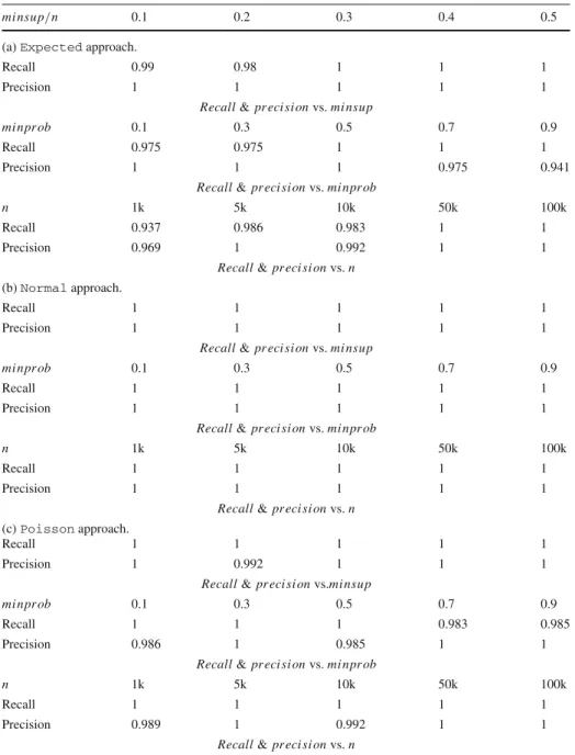
Table 6 Recall and precision of the approximations

mi nsup/n 0.1 0.2 0.3 0.4 0.5

(a)Expectedapproach.

Recall 0.99 0.98 1 1 1

Precision 1 1 1 1 1

Recall&pr eci si onvs.mi nsup

mi npr ob 0.1 0.3 0.5 0.7 0.9

Recall 0.975 0.975 1 1 1

Precision 1 1 1 0.975 0.941

Recall&pr eci si onvs.mi npr ob

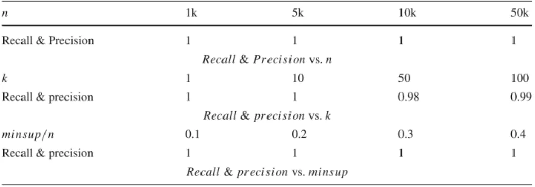
n 1k 5k 10k 50k 100k

Recall 0.937 0.986 0.983 1 1

Precision 0.969 1 0.992 1 1

Recall&pr eci si onvs.n (b)Normalapproach.

Recall 1 1 1 1 1

Precision 1 1 1 1 1

Recall&pr eci si onvs.mi nsup

mi npr ob 0.1 0.3 0.5 0.7 0.9

Recall 1 1 1 1 1

Precision 1 1 1 1 1

Recall&pr eci si onvs.mi npr ob

n 1k 5k 10k 50k 100k

Recall 1 1 1 1 1

Precision 1 1 1 1 1

Recall&pr eci si onvs.n (c)Poissonapproach.

Recall 1 1 1 1 1

Precision 1 0.992 1 1 1

Recall&pr eci si onvs.mi nsup

mi npr ob 0.1 0.3 0.5 0.7 0.9

Recall 1 1 1 0.983 0.985

Precision 0.986 1 0.985 1 1

Recall&pr eci si onvs.mi npr ob

n 1k 5k 10k 50k 100k

Recall 1 1 1 1 1

Precision 0.989 1 0.992 1 1

Recall&pr eci si onvs.n

Apriori algorithm that uses the expected support only [12]; (3) Poisson, the modified Apriori algorithm that uses the Poisson approximation employing the PFI testing method (Sect.5.1); (4)Normal, the modified Apriori algorithm that uses the normal approximation, also employing the PFI testing method (Sect.5.1); and (5)MBP, the algorithm that uses the Poisson approximation utilizing the improved version of the PFI testing method (Sect.5.2).

(i) Accuracy.Since the model-based approachesExpected,PoissonandNormal

each approximate the exact s-pmf, we first examine their respective accuracy with respect to

DP, which yields PFIs based on exact frequentness probabilities. Here, we use the standard

recallandprecisionmeasures [7], which quantify the number of negatives and false posi-tives. Specifically, letMB∈{Expected,Poisson,Normal} be one of the model-based approximation approaches, and letFD Pbe the set of PFIs generated byDPandFM Bbe the set of PFIs produced byMB. Then, the recall and the precision ofMB, relative toDP, can be defined as follows: r ecall= |FD P∩FM B| |FD P| (21) pr eci si on= |FD P∩FM B| |FM B| (22)

In these formulas, both recall and precision have values between 0 and 1. Also, a higher value reflects a better accuracy.

Table6(a) to (c) shows the recall and the precision of the MBapproaches, for a wide range ofmi nsup,n, andmi npr obvalues. As we can see, the precision and recall values are generally very high. Hence, the PFIs returned by theMBapproaches are highly similar to those returned byDP. In particular, we see that theExpectedapproach generally yields the worst results, having precision and recall values of less than 95 % in some setting. The

Poissonapproach performs significantly better in these experiments. Yet in some settings, thePoissonapproach reports false hits, while in other settings, it performs false dismissals. TheNormalapproach is most notable in this experiment. In this set of experiments, the

Normal approach never had a false dismissal, nor did it report a single false hit. This observation also remained true for further experiments in this line, which are not depicted here. In the next set of experiments, we will experimentally investigate the effectivity of the

MBapproach.

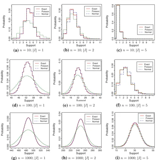
Figure4shows the exact pmf, as well as the pmfs approximated by thePoissonand theNormalapproach, for a variety of settings. In particular, we scaled both the dataset size and the size of the itemsets whose pmf is to be approximated. Since, in this setting, the probabilities of individual items are uniformly sampled in the[0,1]interval, and since due to the assumption of item independence, it holds thatP(I)=_i∈I P(i), a large itemsetI

implies smaller existence probabilities. In Fig.4a, it can be seen that for single itemsets (i.e., large probability values), the pmf acquired by the Poisson approximation is too shallow— that is, for support values close toμI the exact pmf is underestimated, while for support values far from μI, the pmf is overestimated. In Fig.4d, g it can be observed that this situation does not improve for the Poisson approximation. However, this shortcoming of the Poisson approximation can be explained: Since the Poisson approximation does only have one parameterμI, but no variance parameterσ2I, it is not able to differ between a set of five transactions with occurrence probabilities of 1, and five million transactions with occurrence probabilities of 10−6, since in both scenarios it holds thatμI = 5·1= 5·106·10−6=5. Clearly, the variance is much greater in the later case, and so are the tails of the corresponding exact pmf. Since the Poisson distribution is the distribution of the low probabilities, the Poisson assumes the later case, i.e., a case of very many transactions, each having a very low probability. In contrast, the normal distribution is able to adjust to these different situations by adjusting itsσ2Iparameter accordingly. Figure4b, e, h show the same experiments for itemsets consisting of two items, that is, for lower probabilitiesI⊆ti. It can be observed that with lower probabilities, the error of the Poisson approximation decreases,

0 1 2 3 4 5 6 7 8 9 11 0.00 0.10 0.20 0.30 Support Probability Exact Poisson Normal 0 1 2 3 4 5 6 7 8 9 11 0.00 0.10 0.20 0.30 Support Probability Exact Poisson Normal 0 1 2 3 4 5 6 7 8 9 11 0.0 0 .2 0.4 0 .6 0.8 Support Probability Exact Poisson Normal 40 46 52 58 64 70 0.00 0.02 0.04 0.06 0.08 0.10 Support Probability Exact Poisson Normal 10 16 22 28 34 40 0.00 0.05 0.10 0.15 Support Exact Poisson Normal 0 1 2 3 4 5 6 7 8 9 0.00 0.10 0.20 0.30 Support Probability Probability Exact Poisson Normal 440 460 480 500 520 540 0.000 0.010 0 .020 0.030 Support Probability Exact Poisson Normal 200 220 240 260 280 300 0.00 0.01 0.02 0.03 0.04 Support Probability Exact Poisson Normal 15 25 35 45 55 0.00 0.02 0.04 0.06 0.08 0.10 Support Probability Exact Poisson Normal (a) (b) (c) (f) (e) (d) (g) (h) (i)

Fig. 4 Illustration of the approximation quality ofNormalandPoissonfor various settings.a n=10; |I| =1.b n=10;|I| =2.c n=10;|I| =5.d n=100;|I| =1.e n=100;|I| =2.f n=100;|I| =5.g n=1,000;|I| =1.h n=1,000;|I| =2.i n=1,000;|I| =5 Table 7 _{# Itemsets} n Model 1 2 5 10 Normal 0.020 0.078 0.180 Poisson 0.526 0.283 0.077 100 Normal 0.0003 0.0020 0.0134 Poisson 0.0515 0.0283 0.0052

1,000 Normal 2.39E-6 6.12E-6 0.0004

Poisson 5.24E-3 2.85E-3 0.0007

while (as we will see later, in Table7) the quality of the normal approximation decreases. Finally, for itemsets of size 5, the Poisson approximation comes very close to the exact pmf.

(a) (b) (c)

(f) (e)

(d)

(g) (h) (i)

Fig. 5 Accuracy of model-based algorithms versusn.a mi nsup=0.49.b mi nsup=0.50.c mi nsup=0.51.

d mi nsup = 0.49. e mi nsup = 0.50. f mi nsup = 0.51. g p-value, mi nsup = 0.50. h error, minsup=0.50.ierr or,mi nsup=0.50

To gain a better intuition of the approximation errors, we have repeated each of the experiments shown in Fig.4one hundred times and measured the total approximation error. That is, we have measured for each approximationDP∈{Normal,Poisson} the distance to the exact pmf, computed by theDPapproach:

D(M P,D P)=

n

i=0

|M Ppm f −D Ppm f|.

The results of this experiment are shown in Table7. Clearly, the approximation quality of the Normal approach decreases when the size of the itemsets increases (i.e., the probabilities become smaller), while the Poisson approach actually improves. An increase in the database size, is beneficial for both approximation approaches.

The impact of increasing the database size on the individual approximation models has been investigated further in Fig.5. In this experiment, we use a synthetic itemset where each item is given a random probability uniformly distributed in[0,1]. In Fig.5a–c, the average frequentness probabilityPrf r eq(I)that itemIis frequent is depicted for all itemsetsI con-sisting of one item. Since all probabilities are uniformly[0,1]distributed, it is clear thatμI