The copyright © of this thesis belongs to its rightful author and/or other copyright owner. Copies can be accessed and downloaded for non-commercial or learning purposes without any charge and permission. The thesis cannot be reproduced or quoted as a whole without the permission from its rightful owner. No alteration or changes in format is allowed without permission from its rightful owner.
WINSORIZE TREE ALGORITHM FOR HANDLING OUTLIERS IN
CLASSIFICATION PROBLEM
CH'NG CHEE KEONG
DOCTOR OF PHILOSOPHY
UNIVERSITI UTARA MALAYSIA
Awang Had Salleh
Graduate School of Arts And Sciences . . , . . , . . . . . , . . . " . .- , . . UniversiQi utara Malaysia PEliaKUAPd KERJA T E S l S I D l S E R T A S l
(Certification o f thesis / disserlation)
Kami, yang bertandatangan, memperaltukan bahawa (We, the undersigned, cedi@ that)
CH'MG CHEE KEOMG
_ . . ^ .
calon untuk ljazah PhD
(candidate for fhe degree
00
telah mengemukakan tesis / disertasi yang bertajuk:
(has presented his/her thesis / dissetfation of fhe follovjing title):
"WINSORIZE TREE ALGORITHM FOR HANDLING OLlTLlERS IN CLASSIFICATION PROBLEM"
seperii yang tercatat di muka surat tajuk dan kulit tesis 1 disertasi. (as it appears on fhe tifle page and front cover of the thesis /dissertation).
Bahawa tesisldisertasi tersebut boleh diterima dari segi bentuk serta kandungan dan meliputi bidang ilmu dengan memuaskan, sebagaimana yang ditunjukkan oleh calon dalam ujian lisan yang diadakan pada : 03 Ogos 2015.
That fhe said thesis/disserfatfion is acceptable in form and contenf and displays a satisfactory knowledge of fhe field of sfudy as demonstrated by the candidate through an oral examination held on:
August 03,2015.
Pengerusi Viva: . Prof. Dr. Zurni Ornar
(Chairman for VIVA)
Perneriksa Luar: Assoc. Prof. Dr. Mohd Rizarn Abu Bakar Tandatangan
(External Examiner) (Signature)
i
Pemeriksa ~uar: Dr. Wan Rosmanira lsmail Tandatangan(Exfernal Examined (Signature)
Nama PenyelialPenyelia-penyelia: Dr. Nor ldayu Mahat Tandatangan
(Name of Supervisor/Supe~isors) (Signature)
Tarikh:
Permission to Use
In presenting this thesis in fulfilment of the requirements for a postgraduate degree from Universiti Utara Malaysia, I agree that the Universiti Library may make it freely available for inspection. I further agree that permission for the copying of this thesis in any manner, in whole or in part, for scholarly purpose may be granted by my supervisor(s) or, in their absence, by the Dean of Awang Had Salleh Graduate School of Arts and Sciences. It is understood that any copying or publication or use of this thesis or parts thereof for financial gain shall not be allowed without my written permission. It is also understood that due recognition shall be given to me and to Universiti Utara Malaysia for any scholarly use which may be made of any material from my thesis.
Requests for permission to copy or to make other use of materials in this thesis, in whole or in part should be addressed to:
Dean of Awang Had Salleh Graduate School of Arts and Sciences UUM College of Arts and Sciences
Universiti Utara Malaysia 06010 UUM Sintok
Abstrak
Pepohon pengelasan dan regresi (CART) direkabentuk untuk meramal atau mengelas objek dalam kelas yang telah ditentukan daripada suatu set pembolehubah peramal. Namun, kewujudan unsur pencilan mampu menjejaskan struktur CART, ketulenan dan ketepatan peramalan dalam pengelasan. Sebahagian penyelidik memilih melakukan kaedah pra-pencantasan atau pasca-pencantasan pada CART untuk mengendali unsur pencilan. Kajian ini mencadangkan algoritma pepohon pengelasan
terpinda, dikenali sebagai pepohon Winsorize berdasarkan taburan kelas dalam set
data latihan. Pepohon Winsorize menyiasat semua unsur pencilan yang mungkin
dalam data dari nod ke nod sebelurn memeriksa ritik pembelahan untuk mendapatkan nod dengan ketulenan tertinggi. Batas atas dan batas bawah plot kotak telah
digunakan untuk mengenal pasti unsur pencilan dengan nilai ekstrem melebihi Q
*
(1.5xJulat antara kuartil). Data pencilan yang telah dikenalpasti akan dineutralkan
menggunakan kaedah Winsorize manakala indeks Gini Winsorize kemudian
digunakan untuk menghitung kecapahan dalam kalangan taburan kebarangkalian bagi nilai peramal yang disasarkan sehingga kriteria henti ditemukan. Kajian ini menggunakan tiga petua henti: nod yang telah mencapai 10% minimum daripada
jurnlah set latihan, nmi,, nod yang mengandungi 70% atau lebih kehomogenan dan
indeks Gini Winsorize terhitung antara dan di antara pembolehubah adalah 70% atau
lebih. Keputusan yang diperolehi daripada tujuh (7) set data sebenar menunjukkan
bahawa pepohon Winsorize merekodkan kadar ralat yang sama atau lebih rendah
berbanding pepohon tradisional dan pepohon tercantas dalam semua kes terutamanya yang melibatkan pembolehubah yang banyak. Kaedah ini menawarkan proses pengelasan yang lebih baik dengan menyiasat dan mengendali unsur pencilan dalam semua nod. Justeru, sebarang proses pencantasan akan dihentikan apabila kriteria
henti dipatuhi. Pepohon Winsorize menghasilkan struktur pepohon paling ringkas dan
menggunakan bilangan pembolehubah yang sedikit dengan kadar ralat yang rendah.
Pepohon Winsorize menawarkan sokongan untuk melaksanakan pengelasan kepada
pengamal baru dan pengamal berpengalaman mungkin mendapati kaedah ini
memudahkan tugas pra pemprosesan dan analisis.
Kata Kunci: Pepohon pengelasan, Data pencilan, Indeks Gini Winsorize, Algoritma
Abstract
Classification and Regression Tree (CART) is designed to predict or classify the
objects in the predetermined classes from a set of predictors. However, having outliers could affect the structures of CART, purity and predictive accuracy in classification. Some researchers opt to perform pre-pruning or post-pruning of the CART in handling the outliers. This study proposes a modified classification tree algorithm called Winsorize tree based on the distribution of classes in the training dataset. The Winsorize tree investigates all possible outliers from node to node before checking the potential splitting point to gain the node with the highest purity of the nodes. The upper fence and lower fence of a boxplot are used to detect potential outliers whose
values exceeding the tail of Q
*
(1.5xInterquartile range). The identified outliers areneutralized using the Winsorize method whilst the Winsorize Gini index is then used to compute the divergences among probability distributions of the target predictor's values until stopping criteria are met. This study uses three stopping rules: node
achieved the minimum 10% of total training set, nmi,, node contains 70% or above of
homogeneity, and the computed Winsorize Gini purity index within and between
variables is equal or greater than 70%. The results obtained from seven (7) real
dataset indicate that the Winsorize tree scores equal or lower error rates than the traditional and pruned trees in all cases especially when dealing with many variables. This method offers a better classification process by investigating and handling the outliers in all nodes. Therefore, it does not require any pruning process as it stops once the stopping criteria is met. The Winsorize tree produces the simplest tree structure and it typically uses fewer variables with a low error rate. It offers some assistance for performing classification to new practitioners and experienced practitioners may find this method simplify preprocessing and analysis tasks.
Keywords: Classification tree, Outliers, Winsorize Gini index, Winsorize tree algorithm
Acknowledgement
I would like to express my sincere appreciation to Dr Nor Idayu binti Mahat for her
valuable effort, guidance, patience, support and encouragement in supervising this work. Warms thanks to Prof. Madya Dr Sharipah Soaad Syed Yahaya and Dr Nazrina Aziz for providing valuable information regarding to statistics.
I would like to thanks the various people in School of Quantitative Science, Universiti
Utara Malaysia as they provided me a very useful and helpful assistance.
Special thanks to the librarians who are always willing to lend their hands to get my requested books and articles. Thanks to Ch'ng Li Guat for rescuing me in computer problems.
I am grateful to all my friends for cheering me up the working room and thanks to them for the friendship, caring and entertainment.
This study would not have been possible without financial support. I would like to
thank the JPA and SLAI which has supported me during my study. Also, thanks are addressed to Universiti Utara Malaysia for giving me the opportunities in completing my works.
The appreciation also goes to my parents, Ch'ng Seow Khin and Tan Pheik Sim, my family members and my wife, Low Joon Khim for their emotional supports, love, motivation and caring during my study. This thesis is dedicated to them. Thanks in million again to all for providing me a loving environment.
Table
of Contents
Permission to Use ... i. .
Abstrak ... 11...
Abstract...
111 Acknowledgement ... iv Table of Contents ... v ... List of Tables...
viil List of Figures...
xiList of Appendices
...
xvList of Abbreviations ... xvi
CHAPTER ONE INTRODUCTION
...
11.1 Introduction
...
11.2 Examples of Classification Problem
...
21.3 Classification Rules
...
31.3.1 Elements of Decision Tree ... 4
1.3.2 Construction of Decision Tree ... 7
1.4 Classification and Regression Tree (CART)
...
81.5 Challenges in Contructing a Classification Tree ... 10
1.6 Problem Statement ... 14
1.7 Research Objectives ... 17
1.8 Significant of Study ... 18
1.9 Scope of Study ... 19
1.10 Thesis Organization ... 20
CHAPTER TWO LITERATURE REVIEW
...
222.1 Introduction ... 22
2.2 Classification Rule
...
222.3 Parametric Approaches
...
232.3.1 IVdive Bayes Method
...
23 2.3.2 Regression...
2 4.
.
2.3.4 Linear Discriminant Analysis
...
262.3.5 Advantages and Disadvantages of Paramentric Approa'ches
...
282.4 IVonparametric Approaches
...
292.4.1 Neural Network
...
282.4.2 Decision Tree
...
302.4.3 Advantages and Disadvantages of Nonparametric Approaches
...
322.5 Evaluating Rules
...
322.5.1 Types of Error Rate
...
342.5.1.1 Bayes Error Rate
...
342.5.1.2 Achievable Error Rate
...
342.5.1.3 Conditional Error Rate and Unconditional Error Rate
...
352.6 Estimating Conditional Error Rate
...
362.6.1 K-fold Cross Validation
...
342.6.2 Leave One Out Cross Validation
...
372.6.3 Validation Set
...
3 7 2.6.4 Jackknife...
3 8 2.6.5 Bootstrap...
38 2.7 Pre-processing...
40 2.8 Outliers...
40 2.8.1 Outlier Detection...
42 2.8.2 Outlier Handling...
.
.
...
54 2.9 Classification Tree...
56 2.1 0 Pruning Methods...
5 9 2.1 1 Pre-processing and Its Drawback...
63CHAPTER THREE METHODOLOGY
...
....
...
673.1 Introduction
...
7 1 3.2 Framework of Study...
723.2.1 Data Inspection
...
723.2.2 Outlier Handling
...
7 4 3.2.3 Gini Purity Measurement and Tree Construction...
763.2.5 Evaluation
...
803.3 Tree Algorithm
...
803.4 Data
...
84CHAPTER FOUR ANALYSIS
...
864.1 Introduction
...
8 6 4.2 Identifying Percentage of Homogeneity for Stopping Rules ... 874.3 Case 1: Classification in Breast Tissue Data
...
934.3.1 The Statistical Background of the Breast Tissue Data
...
944.3.2 The Construction of Winsorize Tree for Breast Tissue Data ... 99
4.3.3 The Evaluation of Winsorize Tree for Breast Tissue Data
...
1084.4 Case 2: Classification in Egyptian Skull Data
...
1104.4.1 The Statistical Background of Egyptian Skull Data
...
110... 4.4.2 The Construction of Winsorize Tree for Egyptian Skull Data 114
...
4.4.3 The Evaluation of Winsorize Tree for Egyptian Skull Data 120 4.5 Case 3: Classification in Pima Indians Data...
1224.5.1 The Statistical Background of Pima Indians Data
...
1234.5.2 The Construction of Winsorize Tree for Pima Indians Data ... 126
4.5.3 The Evaluation of Winsorize Tree for Pima Indians Data
...
1334.6 Case 4: Classification in Iris Data
...
1354.6.1 The Statistical Background of Iris Data
...
.
.
...
1364.6.2 The Construction of Winsorize Tree for Iris Data ... 138
4.6.3 The Evaluation of Winsorize Tree for Iris Data ... 143
4.7 Case 5: Classification in Bumpus Sparrow Data
...
1454.7.1 The Statistical Background of Bumpus Sparrow Data ... 145
4.7.2 The Construction of Winsorize Tree for Bumpus Sparrow Data
...
1494.7.3 The Evaluation of Winsorize Tree for Bumpus Sparrow Data ... 159
4.8 Case 6: Classification in Indians Liver Patient Dataset (ILPD)
...
1604.8.1 The Statistical Background of Indians Liver Patient Dataset (ILPD)
...
1624.8.2 The Construction of Winsorize Tree for Indians Liver Patient Dataset (ILPD)
...
165...
4.9 Case 7: Classification in Kyphosis Data
...
173...
4.9.1 The Statistical Background of Kyphosis Data 174
...
4.9.2 The Construction of Winsorize Tree for Kyphosis Data 177
...
4.9.3 The Evaluation of Winsorize Tree for Kyphosis Data 180
CHAPTER FIVE CONCLUSION AND FUTURE WORKS
...
182 5.1 Introduction...
182 5.2 Achievement of Stopping Rules...
184...
5.3 Conclusion of Study 185...
5.4 Contribution of Study 188...
5.5 Limitation 189...
5.6 Future Works 190 REFERENCES...
191List of Tables
Table 3.1 : Data Description
...
85Table 4.1. Percentage Selection for Stopping Rule
...
89Table 4.2. Frequency Table of Breast Tissue Data Set
...
95Table 4.3. Statistical Description of Breast Tissue Data Set
...
95Table 4.4. Normality Tests
...
99Table 4.5. Outliers in Parent Node
...
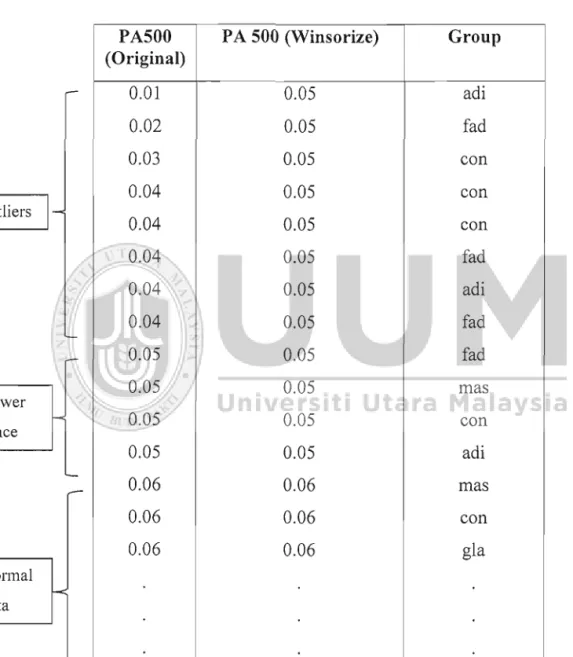
100Table 4.6. Example of Winsorize Data and Gini Purity Index for Variable PA500
...
...
.
.
.
...
101Table 4.7. Splitting point in Parent Node
...
102...
Table 4.8. Number of Observations in Node 2 and Node 3 103 Table 4.9. Splitting Point in Node 2...
104Table 4.10. Numnber of Observations in Node 4 and Node 5
...
105Table 4.11 : Comparison between Traditional Tree, Pruned Tree and Winsorize Tree
...
108Table 4.12. Frequency Table of Egyptian Skull Data Set
...
111Table 4.1 3: Statistical Description of Egyptian Skull Data Set
...
111Table 4.14. Normality Tests
...
1 1 3 Table 4.1 5: Outlier in Parent Node...
114Table 4.1 6: Splitting Point in Parent Node
...
114Table 4.17. Number of Observations in Node 2 and Node 3
...
115Table 4.18. Outliers in Node 2
...
116Table 4.19. Outliers in Node 3
...
116Table 4.20. Gini Index of Winsorize Tree in Node 2
...
116Table 4.21. Gini Index of Winsorize Tree in Node 3
...
117Table 4.22. Numnber of Observations in Node 4, Node 5, Node 6 and Node 7 ... 118
Table 4.23: Comparison between Traditional Tree, Pruned Tree and Winsorize Tree
...
120Table 4.24.Frequency Table of Pima Indians Data Set
...
123Table 4.25. Statistical Description of Pima Indians Data Set
...
123Table 4.26. Outliers in Parent Node
...
127Table 4.27. Splitting Point in Parent Node
...
128Table 4.28. Number of Patients in Node 2 and Node 3
...
129Table 4.29. Number of Outliers in Node 2
...
129Table 4.3 0: Number of Outliers in Node 3
...
1 3 0 Table 4.3 1 : Splitting Point in Node 2...
130Table 4.32. Splitting Point in Node 3
...
130Table 4.33. Comparison between Traditional Tree, Pruned Tree and Winsorize
...
...
133Table 4.34. Frequency Table of Iris Data Set
...
.
.
.
.
... 136Table 4.35. Statistical Description of Iris Data Set
...
1 3 6 Table 4.36. Normality Tests...
138Table 4.37. Outlier in Parent Node
...
139Table 4.3 8: Splitting in Parent Node
...
139Table 4.39. Number of Observations in Node 2 and Node 3 ... 140
Table 4.40. Splitting Point in Node 3
...
141Table 4.41. Number of Observations in Node 4 and Node 5
...
142Table 4.42: Comparison between Traditional Tree, Pruned Tree and Winsorize Tree
...
144Table 4.43. Frequency Table of Bumpus Sparrow Data Set
...
145Table 4.44. Statistical Desccription of Burnpus Sparrow Data Set
...
146Table 4.45. Normality Tests
...
148Table 4.46. Outlier in Parent Node
...
149Table 4.47. Splitting Point in Parent Node
...
150Table 4.48. Number of Observations in Node 2 and Node 3
...
151Table 4.49. Outlier in Node 2
...
152Table 4.50. Outlier in Node 3
...
152Table 4.5 1 : Splitting Point in Node 2
...
153Table 4.52. Splitting Point in Node 3
...
153Table 4.53. Number of Observations in Node 4, Node 5, Node 6 and Node 7
...
155Table 4.54. Outlier in Node 5
...
1 5 5 Table 4.55. Splitting Point in Node 4...
155Table 4.56. Splitting Point in Node 5
...
156 XTable 4.57 Number of Observation in Node 8. Node 9. Node 10 and Node 1 1
...
157Table 4.58: Comparison between Traditional Tree. Pruned Tree and Winsorize Tree
...
158Table 4.59. Frequency Table of Indians Liver Patient Data Set ... 162
Table 4.60. Statictical Description of Indians Liver Patient Data Set
...
162Table 4.61 : Normality Tests
...
165Table 4.62. Outlier in Parent Node
...
166Table 4.63. Splitting Point in Parent Node
...
166Table 4.64. Number of Patients in Node 2 and Node 3
...
167Table 4.65. Number of Outliers in Node 2
...
168Table 4.66. Splitting Point in Node 2
...
168Table 4.67. Number of Observation in Node 3. Node 4 and Node 5 ... 169
Table 4.68: Comparison between Traditional Tree. Pruned Tree and Winsorize Tree Table 4.69. Frequency Table of Kyphosis Data Set
...
174Table 4.70. Statistical Description of Kyphosis Data Set
...
174Table 4.7 1 : Normality Tests
...
1 7 6 Table 4.72. Outliers in Parent Node...
177Table 4.73. Splitting Point in Parent Node
...
178Table 4.74. Number of Observations in Node 2 and Node 3
...
178Table 4.75: Comparison between Traditional Tree. Pruned Tree and Winsorize Tree ...
.
.
.
...
180List
of Figures
Figure 1.1 : Simple Decision Tree
...
5Figure 1.2. Splitting Algorithm of CART
...
9Figure 1.3 : Tree Classifier for Kypliosis (without outlier)
...
13Figure 1.4. Tree Classifier for Kyphosis (with outlier)
...
13Figure 1.5. Tree Classifier for Iris (without outlier)
...
14Figure 1.6. Tree Classifier for Iris (with outlier)
...
14Figure 3.1 : Arrangement of Data Before and After Winsorizing
...
75Figure 3.2. Winsorize Gini Purity Computation
...
70Figure 3.3. Goodness of Split
...
.
.
.
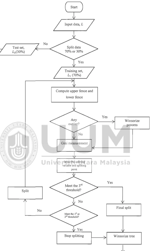
... 78Figure 3.4. Flowchart of Winsorize Algorithm
...
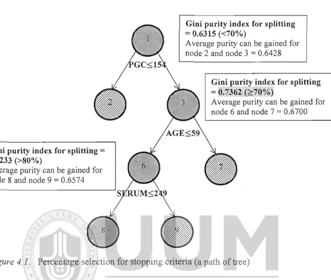
83Figure 4.1 : Percentage Selection for Stopping Criteria (A Path of Tree)
...
92Figure 4.2. Cancer Tissue and Normal Tissue
...
93Figure 4.3(a). Original Data of Variable P
...
:
...
96Figure 4.3(b). Winsorize Data of Variable P
...
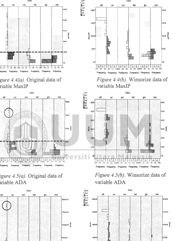
96Figure 4.4(a). Original Data of Variable MaxIP
...
97Figure 4.4(b). Winsorize Data of Variable MaxIP
...
97Figure 4.5(a). Original Data of Variable ADA
...
97Figure 4.5(b). Winsorize Data of Variable ADA
...
97Figure 4.6(a). Original Data of Variable Area
...
97Figure 4.6(b). Winsorize Data of Variable Area
...
97Figure 4.7(a). Original Data of Variable DA
...
98Figure 4.7(b). Winsorize Data of Variable DA
...
98Figure 4.8(a). Original Data of Variable DR
...
98Figure 4.8(b). Winsorize Data of Variable DR
...
98Figure 4.9. Splitting of Parent Node ... 103
Figure 4.10. Child Nodes from Node 2 ... 104
Figure 4.1 1 : Winsorize Tree on Breast Tissue
...
106Figure 4.12. Traditional Tree on Breast Tissue
...
107Figure 4.13. Pruned Tree on Breast Tissue
...
107 Figure 4.14(a). Original Data of Variable nh...
1 1 2Figure 4.14(b). Winsorize Data of Variable nh
...
112Figure 4.15(a). Original Data of Variable bl
...
.
.
.
...
112Figure 4.15(b). Winsorize Data of Variable bl
...
1 12 Figure 4.1 6(a): Scatterplot of bh against mb...
,113Figure 4.16(b). Scatterplot of bh against mb using Winsorize Method
...
113Figure 4.17. Child Nodes from Node 1
...
115Figure 4.18. Child Nodes from Node 2 and Node 3
...
117Figure 4.19. Winsorize Tree on Egyptian Skull
...
119Figure 4.20. Traditional Tree on Egyptian Skull
...
119Figure 4.2 1 : Pruned Tree on Egyptian Skull
...
120Figure 4.22(a). Original Data of Variable SERUM
...
124Figure 4.22(b). Winsorisze Data of Variable SERUM
...
124Figure 4.23(a). Original Data of Variable DBP
...
125Figure 4.23(b). Winsorize Data of Variable DBP
...
125Figure 4.24(a). Original Data of Variable AGE
...
125Figure 4.24(b). Winsorize Data of Variable AGE
...
125Figure 4.25(a). Original Data of Variable PGC
...
125Figure 4.25(b). . Winsorize Data of Variable PGC
...
125Figure 4.26(a). Scatterplot of Original Pima Indians Training Data Set
...
126Figure 4.26(b). Scatterplot of Winsorize Pima Indians Training Data Set
...
126Figure 4.27. Outlier Detection using Boxplot
...
127Figure 4.28. Child Nodes from Parent Node
...
128Figure 4.29. Child Nodes from Node 2 and Node 3
...
131Figure 4.30. Winsorize Tree of Pima Indians
...
132Figure 4.3 1 : Traditional Tree of Pima Indians
...
132Figure 4.32. Pruned Tree of Pima Indians
...
133Figure 4.33 : Iris Flower
...
1 3 5 Figure 4.34(a). Original Data of Variable SepalLength...
137Figure 4.34(b). Winsorize Data of Variable SepalLength
...
137Figure 4.35. Original Data of Variable PetalLength
...
1 3 7 Figure 4.36. Outlier Detection using Boxplot...
139Figure 4.37. Child Nodes from Parent Node
...
140Figure 4.38. Child Nodes from Node 3
...
142Figure 4.39. Winsorize Tree of Iris
...
142Figure 4.40. Traditional Tree of Iris
...
143Figure 4.4 1 : Pruned Tree of Iris
...
1 4 3 Figure 4.42(a). Original Data of Variable Total-length...
147Figure 4.42(b). Original Data of Variable Alas-length
...
147Figure 4.42(c). Original Data of Variable Length-bead - length
...
147Figure 4.42(d). Original Data of Variable Length-humerus
...
147Figure 4.42(e). Original Data of Variable Length-keel-sternum
...
147Figure 4.43. Outlier Detection using Boxplot in Parent Node
...
149Figure 4.44. Child Nodes from Parent Node
...
.
.
...
150... Figure 4.45. Outlier Detection using Boxplot Node 2 (left) and Node 3 (right) 151 Figure 4.46. Child Nodes from Node 2 and Node 3
...
154Figure 4.47. Child Nodes from Node 4 and Node 5
...
.
.
... 157Figure 4.48. Winsorize Tree of Bumpus Sparrow
...
158Figure 4.49. Traditional Tree of Bumpus Sparrow
...
158Figure 4.50. Pruned Tree of Bumpus Sparrow
...
158Figure 4.5 1 (a): Indian Liver (Patient) ... 162
Figure 4.5 1 (b): Indian Liver (Control)
...
162Figure 4.52(a). Original Data of Variable Alkphos
...
163Figure 4.52(b). Winsorize Data of Variable Alkphos
...
163Figure 4.53(a). Original Data of Variable Sgpt
...
164Figure 4.53(b). Winsorize Data of Variable Sgpt
...
164Figure 4.54(a). .Original Data of Variable TP
...
164Figure 4.54(b). Winsorize Data of Variable TP
...
164Figure 4.55. Outlier Detection using Boxplot
...
165Figure 4.56. Child Nodes from Parent Node
...
167Figure 4.57. Child Nodes from Node 2
...
169Figure 4.58. Winsorize Tree of ILPD
...
170Figure 4.59. Traditional Tree of ILPD
...
170Figure 4.60. Pruned Tree of ILPD
...
1 7 1 Figure 4.6 1 (a): Normal Spine...
173Figure 4.6 1 (b): Kypho Spine
...
173Figure 4.62. Outlier Detection using Boxplot ... 1 7 5 Figure 4.63(a). Original Data of Variable Number
...
1 7 5 Figure 4.63(b). Winsorize Data of Variable Number...
175Figure 4.64. Original Data of Variable Age ... 1 7 6 Figure 4.65. Original Data of Variable Start ... 176
Figure 4.66. Child Nodes from Node 1 ... 178
Figure 4.67. Winsorize Tree of Kyphosis ... 179
Figure 4.68. Traditional Tree of Kyphosis ... 179
List
of
Abbreviations
ARM CART CHAID EBP HER ESD HMM ID3 ILPD IQR L LOF LOFB-DRF LS MAD MD MDL MED MEP ML MR OR SPu
Association Rule Mining
Classification and Regression Tree
Chi-Square Automatic Interaction Detection Error Based Pruning
Electronic Health Record Extreme Studentised Deviate Hidden Markov Model Iterative Dichotomiser 3 Indians Liver Patient Dataset Inter Quartile Range
Lower Boundary Local Outlier Factor
Extension of Random Forest Least Square Method
Median Absolute Deviation Mahalanobis Distance
Minimum Descriptive Length Median
Minimum Error Pruning Maximum Likelihood Map Reduce
Outlier Region Splitting Point Upper Boundary
List
of
Appendices
Appendix A Breast Tissue (Training and Test)
...
201...
Appendix B Egyptian Skulls (Training and Test) 205
Appendix C Pima Indians (Training and Test)
...
210...
Appendix
D
Iris (Training and Test) 233...
Appendix E Bumpus Sparrow (Training and Test) 238
Appendix F ILPD (Training and Test)
...
241 Appendix G Kyphosis (Training and Test)...
261CHAPTER ONE
INTRODUCTION
1.1 Introduction to Classification
Classification is a scientific process that refers to activities of allocating objects into pre-determined classes. Also, it is attempting to identify to which group or class a new object should belong to. The classification can be distinguished into two types:
unsupervised classlJication and supervised classiJication (Gupta, 2006). Unsupervised
classification refers to the process of defining classes of objects where one usually aims at either identifying some explainable structures among objects or looking for convenient partitions of the collection of objects. Unlike supervised classification, there are no explicit target attribute which associated with the input. Two examples of simple classical statistics method of unsupervised classification are clustering and dimensionality reduction (Ghahramani, 2004). Often, the number of hypothesized
number of clusters ahead of time will be set by the users (Duda, Hart & Stork, 2001).
In contrary, supervised classification is the process of allocating a new object into its predefined class. The concept of supervised classification is as follows: a classification rule that decides to which class an object should be assigned will be constructed based on a set of measurements obtained from the classified objects
(Cunningham, Cord & Delany, 2008). Then, the constructed classification rule will be
evaluated in order to ensure that it is suitable to classify (or to predict) the class of a future object. The interest of supervised classification is to search for the best possible algorithm that will be able to produce a general hypothesis to predict the correct class
of the future objects (Kotsiantis, 2007; Chaovalit & Zhao, 2005). The challenge in
supervised classification is to build a concise and accurate mathematical model that can assign future object into a correct class. They are many type of supervised classification methods such as decision tree, support vector machines, logistic discrimination, nayve Bayes, random forest, neural network, ensembles, perceptron and much more.
This thesis is concerned with the supervised classification thus the discussion throughout this thesis will refer classification as supervised classification.
1.2 Examples of Classification Problem
In business activities, classification approach can be used to explore the behaviour of
buyers (brand loyalty) and to determine market segmentation (Miller, 2005, p. 25 &
26). One may need to understand the buyers' behaviour towards a certain product or brand. Some criteria including salary, marital status, gender and types of occupation may be used to explain one's preference either interested or not interested to purchase a new brand of product. In banking sector, based on the customer profile, the industry is using a particular classifier to evaluate the risk of approving loan (Thomas, Oliver
& Hand, 2005). The well-known classification algorithms were used to investigate the
credit score data sets accurately (Baesens, Gestel, Viaena, Stepanova, Suykens &
Vanthlenen, 2003).
Besides, classification is widely used in medicine. In hospital for example, a doctor is assisted by a systematic rule to claim a survival rate of heart plant patients (Gupta,
2006, p.15). Also, it has been used to classify human chromosomes into its respective
groups (Cwnow & Franklin, 1973). Different types of classifier have been applied to
detect anomaly intrusion in system. The classifier can overcome security threats in computer network and can be used to identify unauthorized use of computer system
(Bahrololum & Khaleghi, 2008). In other areas, decision tree (C4.5) technique is used
in stock management and control (Wu, Lin & Lin, 2006). With the growth of online
information, Joachims (2005) used Support Vector Machine (SVM) for text categorisation where the main goal is to classify documents into fixed number of predefined categories. Meanwhile, K-nearest neighbours algorithm is studied to
diagnose on the Wiscousin-Madison breast cancer (Sarkar & Leong, 2000).
1.3 Classification Rules
Many classification rules have been devoted by researchers such as Fisher discriminant function, decision trees, neural networks, nearest neighbour approaches, logistic discriminant, and nayve Bayes classification. Each rule has its strengths in dealing with various structures of the data, among others include distributions of population i.e. population's distribution, type of variables and correlation among variables. Despite of variety classification rules, the oldest systematic classification
procedure called decision tree has become a focus of interest in this thesis. Decision
tree is a logical model which often represented as a binary tree (two-way split). It shows how the target variable can be predicted using all independent variables. The tree straightforward shows how each independent variable is split, which then lead to the prediction of the target variable. Such interesting feature has made this tool unique
compared to other existing classification tools which commonly explained by mathematical formulae. Like continuous development on most classification tools, this thesis concentrates to investigate the decision tree, often termed as tree, in an attempt to add some values in the methodology of constructing it.
1.3.1 Elements of Decision Tree
In classification problem, the goal of a decision tree is to predict the value of a target
variable, which represented group of objects using some input variables. Figure 1.1
shows a simple decision tree with two splits. A basic structure of a tree includes (i) node and (ii) branch. A tree begins with aparent node (labelled "a") and it splits into two non-terminal nodes (labelled "b" and "c"). The binary split from the previous node is called "branch". For example, parent node "a" produces a branch that contains node "b" and node "c". Each non terminal node will split continuously until it cannot be split due to some predetermined constraints. The node that can be split is termed as non-terminal node whilst the final node which cannot be split anymore is called terminal node or leave, i.e. nodes with labelled "e", "f", "g", "h" and "in.
Figure I. I. Simple decision tree
The structure of tree is simple but produces a powerful form of multiple of variable analysis. It is a flow chart like structure which split from node into branch like segment by its algorithm. There are many types of tree available in practices including ID3 (Iterative. Dichomotomiser 3), CHAID (Chi-squared Automatic Interaction Detection) and CART (Classification and Regression Tree). The difference about these trees lay 'on criteria used in the splitting process. ID3 is a tree based on information theory and attempt to minimize the expected number of comparisons. The first question asked must divide the search into two large domains while the subsequent perform a little division of the space (Dunham, 2003). However, ID3 has many disadvantages where it can only deal with nominal variables, unable to deal with noisy data as it could lead to overfitting tree structure, incapable to handle
missing values, always end up with bushy tree and much more. (see Xu, Wang &
Chen, 2006; Octavian, 201 1). Therefore, C4.5 was devoted to improve the condition
(CHAID) was popularised by Kass in year 1980. It is built for non-binary tree which is used for large dataset.
In comparison to ID3 and C4.5, CHAID performs Chi-square test and F-test for classification and prediction purposes. CHAID is normally used in direct marketing
(Haughton & Oulabi, 1997) and it is said a perfect tool to discover the relationship
between variable (Gilbert, 2010). Another structure of tree called classification and regression tree (CART) has interesting features where it only performs binary split in every single split of tree construction. Such structure supports high speed deployment and considered by many as the most versatile predictive modelling algorithm which produce an accurate prediction. Besides, it may consider various types of variables in a single structure hence makes it as a good choice of tree in many real practices (Loh,
201 1; Breimen, Friedman, Olshen, & Stone, 1984). Therefore, this study sets to focus
more on this type of tree.
In general, CART is much simpler than CHAID and C4.5 as it does not split into multi-ways. Moreover, it will keep on splitting until the specified threshold is met. The splitting process of CHAID might be stopped too early as this method attempts to avoid over fitting. Thus, some of unimportant variables might be masked by important variables. Meanwhile in C4.5, the pruned tree will be just substituted by a branch which caused insufficient of information. And, all errors are treated as equal which in practical application, some errors are might be more serious than the others. Although
decision trees are much easier to be understood, the process of constructing a good, accurate and reliable decision tree is influenced by the data.
1.3.2 Construction of Decision Tree
Decision tree can be learned by splitting data into subset based on the attribute value test. A set of if-then rules is used to improve the human readability. The tree like graph is used for inductive inference. It is said to be robust to noisy data and capable of learning disjunctive expression. It also provides a highly effective structure where it could balance the risks and rewards associated with each possible course of action. The data is split randomly into training set and test set where the former set is used to construct a tree and the latter is used to evaluate the constructed tree. The use of training set and test set will avoid the construction of over-performed tree and will provide a reliable tree for h t u r e classification. The tree is built in accordance with a splitting rule which divide the data into smaller part where the objects from the same class are assigned into the same nodes. This process is repeated on each derived subset by top-down induction of decision tree until each leaf consists of a single
observation (Rokach & Maimon, 2008), and this scenario is referred as maximum
homogeneity (Breimen et al, 1984). Gini index, Entropy, and Twoing splitting rules
are commonly used as a splitting algorithm to separate the objects in every node. Among these algorithms, Gini index is widely used as it works well for noisy data especially in classification tree. This index is computed for each variable and the one with the highest Gini purity index (or lowest Gini impurity) will be selected for the next variable to be split.
Specifically, a tree begins with a parent node, t,. The parent node tp will be spilt into
left (t,) and right (t,) child nodes by using the best splitting value of variable,
xf .
The process of splitting is repeated at both left and right child nodes to produce more child nodes. Such processes are repeated until either a tree or every node reaches a pre-determined threshold. The maximum tree means only one class in the terminal node. However, the maximum tree may turn out to a very huge, complicated and bushy which may have hundred levels. Thus, setting a threshold is needed. In this case, the splitting is stopped when the number of objects in the node is less than a
predefined required minimum,
nmin.
Usually,nmin
is set as 10% (Timofeev, 2004)of the learning sample size. To get the maximum right size of tree, pruning procedure is applied which consider on the optimal proportion between the complexity of tree and the error rate.
1.4 Classification and Regression Tree (CART)
Classification and regression tree (CART) is among the popular classification
methods which proposed by Breimen et al. (1984). This type of tree tackles two types of variable where a classification tree is suitable for categorical dependent variable and regression is suitable when dependent variable is quantitative (Wilkinson, 1992). CART algorithm uses a multistage decision process by completing a set of variables jointly to make a decision. On top, there is a root of tree or called parent node that
would split into binary ways (0 for left split and 1 for right split) which associate with
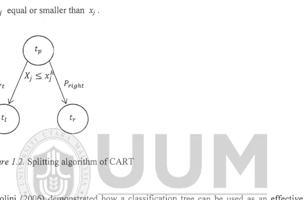
the internal nodes (child nodes). Decision would be made based on the threshold at every level. As depicted in Figure 1.2, objects in the parent node (t,) will be split into
either the right internal node (t,) or the left internal node (tl). Let
xi
be the splittingvalue of the variable
Xi
at t p . The split occurs such that objects in the t, will havevalues of
Xi
greater than the splitting value, xi, and objects in the tl will have valuesof
Xi
equal or smaller than xi .Figure 1.2. Splitting algorithm of CART
Bertolini (2006) demonstrated how
a
classification tree can be used as an effectivetool for quality control practices in oil pipelines. The tree identifies which pipelines to monitor and to choose the most suitable monitoring policies for it. His study was
motivated by Breiman et al. (1984) which suggested that inspection activities and
spillage can be detected or recognised by operating classification and regression trees method. The idea provides a better way to detect the expected spill for cross country oil pipelines although different countries face different types of failures. Breimen et al. (1984) indicated that digit recognition can also be done by using classification and
regression tree (CART). Besides, CART has been used to characterize the long-term
survival after surgery (Valera, Walter, Yokohama, Koyama, Liai & Okamoto, 2006).
Chen, Wang and Zhang (201 1) used tree in biometric and statistical genetics. CART
also applied in medical diagnosis and prognosis. Breimen et al. (1984) used the methods to diagnose heart attacks problem. He tried to classify patients into two different classes: patients who are at risk of dying within 30 days following heart attack (class 1) and the swvivor (class 2). CART is ideally suited for exploring and modelling the complexity in ecology data. De'ath and Fabricius (2000) studied on the ecology data sets using soft coral survey data from Australian central Great Basrier
Reef. They analyze three groups of taxa which are Efflatounaria, Sinularia and
Sinularia Flecibilis. CARTS have been used to analyse the relationship and partition
the response into homogeneous group. Furthermore, CART is also widely used in galaxy classification, financial crisis or defaults, classifying mammals, and so much more.
1.5 Challenges in Constructing a Classification Tree (CART)
In real practices, there is no specific formula to confirm on how good the constructed classification rule is. As the matter of fact, the choice of "good classification rule" depends on the perspective, background, intuition or intention of practitioners in constructing the rule (Jacobs, 2001). Some practitioners aim to have a rule that will give minimum cost of loses rather than a rule with the highest accuracy of classifying objects to their correct group. Some would strongly rely on the accuracy indicators (e.g. error rate and Brier score) where the rule with the highest accuracy is the best choice. Statisticians would evaluate the goodness of classification model based on the mean square error and variance of estimator. Sometime, the priority of choosing a rule is based on the simplest one and much easier to be understood. Statisticians,
economists and medical practitioners put much effort to work with a linear base-rule due to its straight forward process whilst machine learning groups and engineers would prefer on rules that do not rely on any standard assumption such as normality of data. Therefore, there is no exactly the best rule but the process of classification technically searches for the best possible rule.
Outliers are extreme data points which have the potential to influence the statistical
analysis (Evan, 1999; Jacobs, 2001). The occurrence of outliers may due to mistake
made during data entry or in fact valid. Simply ignoring the outliers would destabilise the estimation. Therefore, the whole data must be routinely inspected so that the true colour of the outlier can be defined accurately. Although there are many analytical calculation and graphical displayed tools to spot the outliers, some type of outliers might be masked by several reasons. How if we do not minimise the distortion? And, what would happen to the quality of the data if no action to be taken to such outliers? How the tree structure would be if the data contains outlier? Unreliable output will be generated from the unfiltered data. Outlier may bring a huge effect to some rule's construction. For instance, a slightly different value in the data would create a
different tree classifier. Figures 1.3 to 1.6 are the examples of Kyphosis and Iris data
sets to demonstrate how the construction of trees can be deviated due to the influence of outliers. Ignoring such outlier problem may result in wrong estimated values hence producing different structure of trees. At worst, a future object may be allocated to an incorrect class.
In the Kyphosis data set, three variables are used to classify objects into two levels of kyphosis (a type of deformation) either absent or present after the operation. The constructed trees based on data without outliers (Figure 1.3) and with outliers (Figure 1.4) indicate that different trees have been constructed due to the influence of outliers though the same variables have been chosen in the tree construction. Sometimes, the existing of outliers may influence the choice of variable to be split. In the example of
Iris data set as shown in Figure 1.5 and Figure 1.6, the outliers reflect the changes on
the parent node. The examples given give a sign that somehow outliers may influence the structure of the constructed tree.
The possible challenge in this problein is that the object might be misclassified into a wrong group. Figure 1.3 and Figure 1.4 demonstrate the classification process on
Kyphosis data set. The data have three independent variables (Age, S t a r t ,
Number) and a dependent variable (type of deformation) with two states, absent or present after the operation. Figure 1.3 shows the constructed tree without outliers while Figure 1.4 shows the tree with outliers. Both trees have different structures on the left split due to the present of outliers. Although the outlier is small, it may give some impacts on the structure of the tree, the splitting points and future classification.
If a future object has criteria with Age = 36, St art = 1 1, Number = 3, then tree in
Figure 1.4 will assign such object to group of present but tree as in Figure 1.3 will identify it as absent. For this reason there is a need to properly address the occurrence of outliers in a tree.
Commonly, measuring the accuracy of a constructed tree can be done by taking the error rate and the cost of error. But, the latter is sometime hard to achieve as prior information or expertise knowledge is required.
Start 14.5
rS
I I Aue ~1157.5 1
Figure 1.3. Tree classifier for Kyphosis (without outlier)
Starl f 12.5
I
virg~n~ca virginica
Figure 1.5. Tree classifier for Iris (without outlier)
Petal Len h 4.95
ST-
~~lal.~en$Ih < 4.?5Sepal.Le 5.15 virgi11,ica virpinica vers~coIor vers~color
Figure 1.6. Tree classifier for Iris (with outlier)
1.6 Problem Statement
Sections 1.3 and 1.4 have given a general idea about CART and some challenges on
constructing such type of tree have been highlighted in Section 1.5. Unawareness towards the existence of outliers can cause a misguidance to the future cases as the
constructed model is bias and inaccurate to present the behaviour of actual
information (Tabia & Benferhat, 2008). Thus, many researches have been carried out
to solve the problem in classification. The first approach is to depend on the tree itself to isolate the outliers from process of splitting the data during tree construction. This approach was implemented by Breimen et al. (1984) and Shouman, Turner and
Stocker (201 1). Then, the tree is pruned accordingly to reduce the complexity of the
tree classier and hence improves the predictive accuracy by the reduction of overfitting. However, using all the data may lead to a bias and bushy decision tree
(John, 1995; Engels & Theusinger, 1998). Thus, pruning the constructed tree would
be a good option. Although pruning process could produce an accurate tree with balance size of tree, but this method requires pruning knowledge and experience. It demands users with some statistical or analytical knowledge, but could be troublesome to practitioners. Therefore, some researchers prefer to perform a pre-
processing before constructing a tree (Reif, Goldstein, Stahl & Breuel, 2008; Kyung,
June, Dao & Nam, 201 1; Han & Kamber, 2006). In pre-processing phase, graphical
tools such as Boxplot and probability plot would be used to identify outliers in the data. Once the outliers are determined, then the next step is to critically handle them. Eliminating the outliers is easy but it produces "clean data set" which will definitely
provide us a "good classifier". As pictured in Figure 1.3 to Figure 1.6, few outliers
can cause a tremendous bias split to the whole structure of tree classifier. Sometimes,
this phenomenon will be even worse when some of the explanatory variables are
masked by the outliers. It means that the "extreme value" might hide some variables to be split. Therefore, this method could be a risk if the tree contains bias split as
wrong classifier might provide wrong prediction to us. John (1995) has introduced an idea of pruning and reconstructing tree. The branches of tree will be pruned at the first time to eliminate the outliers. Then, the tree will be reconstructed in order to get the fitted tree. Despite of promising and unbiased tree, the idea faces with some drawbacks as it demands for double tasks to prune and reconstruct the tree. Besides,
many data could be lost due to outliers' termination. Wang, Gu and Wang (2004)
suggested another idea that developing a tree by starting with the most insensible attribute (the attribute that give the less important in classification). As the tree growth, the most sensible (most important attribute) will be chosen hence the outlier will be isolated in some nodes at the bottom of the tree. Yet, this idea has received little attention from other researchers
Considering the weaknesses of earlier idea or approaches, this study initiates the idea of reducing the effects of outliers using a method called Winsorize, which commonly used to compute robust statistics e.g. mean, standard deviation and etc. The idea of winsorizing is to set all the outliers to a specified percentile of the data. However, the choice of percentile is subjective. Too low percentile will allow the outliers to be included in the tree construction but too high percentile will lead to small variance of measurements but high bias to the tree. The idea of when to accommodate outliers is another issue to debate. If one performs Winsorize on the data prior to construction of a tree, then we will miss out to see the state of outliers in a tree. Such phenomenon happen because the outliers have been replaced with the percentile before the classification is taken place. To allow a tree that represents the actual data, this study
proposes to have simultaneous processes of detecting and winsorizing outlier as well as nodes splitting. We winsorize the data when the outlier is found so that the splitting
algorithm namely Gini index can be computed without the influenced of the detected
outliers. Then, we split the original data using the estimated Winsorize Gini Purity
Index. This proposed strategy will promise a splitting process that is not biased
towards skewed data which lead to produce full unbiased structure of tree. This structure will explain about the data and will be useful for future data especially when the future data also contain outliers.
Selecting the right variable and the splitting point are important in order to get a maximum homogeneity in every single split. The maximum homogeneity of left and right child node from previous node is equivalent to the change of impurity
function,Ai(t)
.
It means that the objects which have the similar behaviour areassigned into their own group. However, the outliers would just affect the purity and cause to a bias structure of tree at the end. Therefore, the process of constructing a tree that is not sensitive towards outliers needs to be outlined. This study is looking for the best possibility to the tree structure.
Generally, tree is allowed to split as bushy as it could in order to achieve maximum homogeneity. Then, the tree is pruned based on the tolerant error rate. However, this could lead to time consuming. Alternative to this practice, this study suggests to stop the splitting process before over fitting tree is obtained.
1.7 Research Objectives
This study proposes a new algorithm of tree that insensitive towards the outliers. Therefore, the research objectives of this study are:
1. To determine outlier in a data prior to construct the branch of tree.
2.
To manage the identified outliers accordingly using Winsorize method.3. To integrate the process of determining outlier and identifying outliers with the recursive process of constructing a tree
4. To propose stopping criteria in constructing tree in order to avoid an over-fitting tree.
5 . To compare the new Winsorize tree with the traditional trees.
1.8 Significant of Study
This study provides an alternative classification rule based on decision tree suitable to handle the contaminated data. It offers a data cleaning process embedded in the classification process, which is better than common practices that clean the data prior to the classification. Such simultaneously processes may highlight outliers in the classification, identified by the simple information extracted from a box plot at each investigated node. Next, the proposed Winsorize Gini purity index offers an unbiased way to deal with selection of information variable for splitting. Whilst, the stopping criteria suggested in this study may assist on constructing a tree at optimum level without waste.
In practice, sometimes a practitioner may have some doubts with the data in hand especially when outliers are detected. Some outliers occur due to mistake in data
entry, measurement error or in fact valid. Simply ignoring or terminating the suspected values could be a risk which might cause violation to the end result. Therefore, this study provides a process which insensitive towards outliers making the computed error rate less biased. Overall, the proposed tree construction strategy ensures a quality data used for data mining, which will be helpful for practitioners or researchers whom are less proficient with tree methods.
1.9 Scope of Study
This study focuses on the problem of constructing decision tree for classifying objects into one of two groups when a sample is contaminated with outliers. Current practices need practitioners to clean the data before a construction of tree. Such practice demands a practitioner to master the arts for cleaning the data to avoid over-cleaning which may end up with over performance in classification. Besides, the choice of tool for identifying outliers may not comply with the aim of classification, to minimize the error for future data. In fact, some practitioners might be too relying on the tree itself as it could isolate the outliers into separated nodes. However, this scenario might end up with a bushy tree and some important variables might be masked. This study aims on improving such practices by performing the process of data cleaning and construction of a rule simultaneously to offer much convenience and reliable used among practitioners. However, detection of outliers was set among the continuous variables rather than categorical variables. The continuous data is sorted and the suspected value according to the preceding and succeeding values is then examined. The detected outlier will be penalised before performing the Gini measurement for
splitting. Although there are various types of trees, this study uses the CART which performs as binaly split. This tree could perform classification with multi-type of variables, thus make it as a convenience tree for practices.
1.10 Thesis Organization
This thesis focuses upon the problem of the outliers while constructing the tree to obtain a more reliable and accurate tree. This chapter describes the background of tree and highlights the problem facing in the method when dealing with outliers. Also, this chapter mentions about the contribution towards the body of knowledge in both academic and industrial.
Chapter two of this thesis reveals the parametric and nonparametric models in classification. It draws the attention on why the previous classification tree method is not performed well when dealing with outliers in the data. Also, the chapter discusses some outliers detection and handling methods which have been widely used since few decades ago. Besides, tlie research gaps, the benefits and drawbacks of trees are also illustrated in details in this chapter.
The foundation of the proposed method is displayed in chapter three where it examines the previous works and improving in the algorithms and arithmetic in Winsorize Gini index measurement, which contribute to more accurate and precise result in both classification and prediction. These will be the base for the contribution of this study. Besides, the data descriptions are also presented.
Chapter four shows all the results collected from the designed tree on some existing data sets, using the designed research methodology. Comparison between traditional trees, traditional pruned tree and the proposed tree were performed to give evidence that the proposed tree is comparable, and sometimes better than the established tree designs.
The last chapter gives the summary of the study, contributions, limitations, recommendations and possible future works. The successful accomplishments of research objectives are also explained.
CHAPTER TWO
LITERATURE REVIEW
2.1 Introduction
This chapter overviews some existing classification rules and the outlier identifiers, the strengths and weaknesses of each method are highlighted.
2.2 Classification Rule
The general term of classification is a process of assigning the objects into their group or category. Before the technical specific methods for classification, people classified the object based on their intuition. Those having the same behaviour or characteristics would be assigned into the same group. However, the intuitive decision would create a serious problem as different people have different intuition. Classification rules have been successfully implemented to solve the real world problem (Mahat, 2006).
Freitas (2014) indicated that classification normally uses prediction rules to express
knowledge. IF-THEN rules are used in prediction rules with the condition to produce
y, a label given to class or group. If all the condition in antecedent rule are satisfied
then the prediction of the goal attribute will be satisfied the consequent rules. With a few conjunctions of if-then rules, the relation between the attributes can be narrowing down. This knowledge is useful and intuitively comprehensive for most users.
2.3 Parametric Approaches
Generally, parametric base classifiers are powerful statistical methods that enable to produce an accurate and precise estimation providing that normality assumptions are satisfied. In contrast, nonparametric methods do not require any normality assumption for parameter estimation.
The parametric test often refers to classical or standard test that makes assumptions about the parameter of the population from the selected samples. Some of the parametric approaches include:
2.3.1 Na'ive Bayes Method
Bayes method is a key technology that has been used for classification purposes after
it was proposed by Bayes (1702-1 76 1). Bayes approach to statistics attempts to fully
utilise the available information in order to reduce the uncertainty so that a better decision can be made. The uncertainty means unknown outcomes of various situations. The expression of "it is probable", "the chances are" and so on are always used to deal with the uncertainty condition. When such expressions are quantified, it means one is dealing with "probabilities". Let P ( A ) and P ( B ) refer to the probability
that event A will occur and event B will occur. P(A1B) is the conditional case which
refers to the probability A would happen given that B has already happened. Then, the
Bayes theorem is
P(A.IB) = P ( B J A ) P ( A ) / P ( B ) (2.1)
P(A.
I
B ) = the probability of the object B belonging to class A.P ( B IA) = the probability of obtaining the attribute values B if we know that it belongs
to class A.
P ( A ) = the probability of any object belongs to class A without any other information.
P ( B ) = the probability of obtaining the attribute values B whatever class the object
belong to.
This method is not sensitive to irrelevant variable, it can handle real and discrete data, more accurate as prior class probability is used and handles stream data well. However, this method has been criticised as it requires us to specify a prior distribution for all the unknown parameters. In many cases, the prior knowledge is vague, unclear, or non existent thus making it extremely hard to specify a value for
the model (Duda & Hart, 1973).
2.3.2 Regression
Regression is a statistical method used to describe the nature of relationship between independent variables and a dependent variable. The relationship can be positive or negative, linear or nonlinear. Whilst, coi-relation is used to determine the relationship
between the two variables ( x , y ) (Bluman, 2004, p. 495; Larson & Farber, 2006, p.
458; Abraham & Ledolter, 2006). A positive relationship means that either variables
increase or decrease at the same time whereas a negative relationship means one variable increases but the other decreases and vice versa (Blurnan, 2004). The simple linear regression consists of only one independent variable corresponds to one
dependent variable. In the multi-linear regression, there is only one dependent variable but several in independent variables.
The equation of linear regression can be written as
i. Simple linear regression
. .
11. Multiple linear regression
Y =
P I X I
+
P 2 ~ 2+ ' ' ' +
Pnxn+
PO-
This method can help us to predict the value of one unknown variable through one or more predetermined variable(s). When the relationship between the independent variables and dependent variable are linear, it shows an optimal result. However, linear regression is often inappropriate for non linear relationship. Besides that, the output is only limited to numeric value. The implementation of regression for classification can be done by discretising the numeric dependent variable such that
values lower than a threshold belong to class 1, and the remainings to class 2.
However, such exercise will be troublesome is the classification involves more than two classes. Further discussion relating to this idea can refer to (Grop, 2003, p. 33;
2.3.3 Logistic Regression
Logistic regression is another parametric approach that resembles linear regression. In multiple logistic regressions, it describes the relationship between one dependent
variable and several independent variables (covariate). What distinguishes a logistic
regression from linear regression is that the output is in binary or dichotomous. Individuals whose predicted value probability is more than 0.5 will be assigned to
group 1; otherwise to another group. The assumption here is each observation, yi
comes from Bernoulli distribution with E ( y ) = P ( y = 1). The specified form of
logistic regression model can be written as
Logistic regression has several advantages over the linear regression in classification. For instance, normal distribution assumption is not required in independent variables. It does not assume linear relationship between independent variables and the dependent variable. Besides that, independent variables can be in mixed variables. Unfortunately, in order to get a meaningful and stable result, it needs more data and it might be costly. Other work can be obtained in Hosmer and Lemeshow (2000).
2.3.4 Linear Discriminant Analysis
Linear discriminant analysis was devised by Fisher in year 1936 with the main idea of finding projection to a line which the samples from different classes can be well separated. It also seeks to reduce the dimensionality. Consider assigning an object
with measurement vectors
x
consisting p variables to either class G,orG2.
A functionf (x) of the measurements is used to compare with the threshold to decide which class
of the object is classifying to, G,if f (x) is greater than the threshold and to G2
otherwise.
Seeking a scalar y by projecting the sample
x
onto a line y = w T x . Of all thepossible line from each point to the line, select the one with the maximum separability. Measurement of the separability is needed to find the good projection
vector. If the means of
x
in Gland G2 are pland p2 then the mean of y in GI and G2can be written as w T p l and w T p 2 respectively. Assuming the covariance matrix, C
from both group are the same then the variance of Y is w T z w in both group and the maximum w is
The parameters pl, p2 and C are usually unknown, thus the estimated parameters are
used to replace it. For instance, p1 is replaced by T, and C is replaced by S the
estimated pooled-covariance matrix. Then the distance measure between two groups is
The best value of w is to choose the maximize D (w) which is given by s-'(xl - x 2 )
. There, y = w T x can be written as y = (Zl - x~)s-'x. Allocation of an object to
GI if y is closer to
y1
= (Z1 - X ~ ) S - ~ X ~ and to G, withy2
= (xl - X ~ ) S - ~ X ~otherwise. Further discussion on this topic can be found in Lachenbrunch (1975) and Mclachlan (2004).
2.3.5 Advantages and Disadvantages of Parametric Approaches
Generally, parametric modelling has been widely applied to solve real world problems. It is based on the probability distribution which normal distribution is the most common. And, the samples from different groups are independent and the
variances are equal between groups. If all the assumptions are satisfactorily then
parametric methods produce high accuracy of estimation. The training sites are reusable and it generates information classes. Besides, parametric test is also more powerful than non parametric test when dealing with continuous variables.
However, this approach contains some drawbacks. Parametric is not strong enough when particular assumptions are not met or violated. In addition, we need to consider the cost and difficulties of selecting the training site and the signature homogeneity of information classes might also varies. Moreover, it is only reasonable to apply parametric approach if the samp