AN INVESTIGATION ON THE DEFLECTION ESTIMATOR MODELS IN LASER FORMING OF THE FULL CIRCULAR PATHS

Corresponding Author: Rasoul Tarkesh Esfahani

,

CODEN (USA): JCRSDJ

2014, Vol. 2, No. 2, pp:268-276 Available at www.jcrs010.com

ORIGINAL ARTICLE AN INVESTIGATION ON THE DEFLECTION ESTIMATOR MODELS IN

LASER FORMING OF THE FULL CIRCULAR PATHS Rasoul Tarkesh Esfahani*, Sa'id Golabi

Faculty of Mechanical Engineering, University of Kashan, Kashan, Iran

ABSTRACT: In this paper, the linear and non-linear deflection estimator models in laser forming of full circular scan paths are studied. Firstly, regarding the Taguchi design of experiment method, some simulations are performed with the verified finite element model. The model is then studied with two groups of linear and non-linear models with different assumptions. Finally the best model type is selected by comparing the results of different models' mean error values. It is concluded that, regarding the limitation of the used models' training data, the error value of the linear model with the assumption of the independency of the models and in separated number of the scan radii is less than the other models. The difference between the mean error values of the first and second best models is about 44%.

KEYWORDS: Laser forming, Circular scan path, Finite Element analysis, Taguchi method, Optimization. INTRODUCTION

The laser forming process is one of the advanced forming processes of the sheet metals which is widely employed for ship manufacturing, automobile manufacturing, microelectronics and airplane manufacturing. In this process, the sheet metal is formed using the non-uniform thermal stresses. Comparing to the other common sheet metal forming processes, the laser forming has several advantages including the lower manufacturing costs, shorter production time and higher precision in small manufacturing volumes. Forming of the complex contours with curved profile and manufacturing of small work pieces are also possible in this process. Furthermore, it is possible to form brittle materials such as titanium alloys, nickel alloys and ceramics (Shi et al., 2006) Since the available numerical simulations are time consuming on the one hand, and the solution of the analytical models is hard and their results are not satisfactory on the other hand, therefore the models which can estimate the correct estimations in shorter solution time and with better accuracy are the matter of interest. Scully, (1900); Geiger et al., (1993); Geiger et al., (1995) and Yau et al., (1998) suggested that the bending angle could be calculated as a function of the path energy. Therefore they employed a least square estimation to develop a model for the bending angle as a function of the path energy. However, since the variance analysis in Cheng and Lin work is shown that some other parameters like the beam diameter, the sheet metal thickness and length also significantly affect the bending angle, therefore Cheng and

Lin, (2000) have suggested that the bending angle could be determined as a function of the volume energy instead of the path energy. Similarly, the least square estimation is employed for development of the regression model for the bending angle as a function of the volume energy. The comparison between the volume energy and path energy functions in the work of Cheng and Lin showed that the volume energy function estimates the bending angle more accurately in comparison with the path energy function (Cheng and Lin, 2000).

In the research of Shekhar Chakraborty et al., (2012), a non-linear regression analysis was carried out according to the data obtained from experiments using the Minitab professional software. The objective of the analysis was develop an equation to relate the desired output (i.e. bending angle) to all of the input parameters in laser forming in the domain of the studied parameters. The derived equation is as follows. They also used this equation for production of excessive data for training of their neural network. In which P, v, d, r and n are the laser beam power, the laser beam scan speed, the laser beam diameter, the position of the laser beam scan and the number of the laser beam scan passes respectively.

Hosseinpour Gollo et al., (2011) performed a regression analysis on the laser forming parameters for prediction of the sheet metal bending angle. Regarding the parameters' domains that they supposed in their research, in addition to the parameters such as beam power, beam diameter, scan speed, sheet metal thickness and the number of the scan passes;

they taken into account two additional parameters: the material and the beam's radiation pulse duration. They showed that the results of the prediction using a second order polynomial had the best agreement with the experimental results. Their equation is as follows: Where M, P, V, S, T, N and D are the material parameter (the two materials: ST12 and AISI 304), the laser beam power, the beam scan speed, the beam diameter, the sheet metal thickness, the number of the scan passes and the beam pulse duration respectively.

Cheng and Lin, (2000) employed three supervised neural networks for prediction of the laser bending angle using the experimental data. A group of the experimental data was employed for training of the networks, while another group was used for models' performance evaluation. They concluded that the neural networks are quite faster and in comparison with the multivariate regression analyses, the neural networks are easier. In another work of Chen et al., (2002), a new hybrid fuzzy neural network was proposed for prediction of the bending deformation of the sheet metal by laser. The main characteristics of this model were the fuzzy rules and the fuzzy membership functions which can be improved directly and automatically. This is a perfect characteristic for prediction and control of the complex systems. Shimizu invented a method by which the decision making on the laser paths, laser power and scan speed for forming of a simple dome shape using genetic algorithms could be carried out (Shimizu, 1997).

A genetic algorithm based approach for studying the probability of using this algorithm in laser forming was presented by Cheng and Yao, (2004) and some shapes with 2D profiles was selected accordingly.

Maji et al., (2013) presented some soft computing based methods to predict the deformations produced by laser forming. The deformations are assumed to be functions of the laser thermal parameters and the direct radiation paths of the laser for obtaining a desired shape. They employed the genetic algorithm neural network and adaptive neural network-fuzzy interface system in their research. The beam power, scan speed, the laser beam diameter and the number of scans are the input parameters to their model, and the bending angle is the output parameter. Both of the employed methods is shown to be able to predict the bending angle satisfactorily. Therefore, both of the models can be employed to provide comparable predictions in inverse analysis for developing a relation between the

produced shape and the laser forming process parameters.

Mahdi Asadollah, (2013) implemented an intelligent system for production of the complex shapes on the metal strip. In the first step, they studied the effect of the different laser forming process parameters on the resulting bent strip using finite element simulation. Then they trained an appropriate neural network to access the information and predict the result of the forming process using different laser parameters. Finally, they implemented a program for optimization of the different developed functions using genetic algorithm. The program suggested the laser forming parameters so that the operator can form the desired profile with appropriate accuracy and lower laser energy consumption. The developed algorithm intelligently determined the laser input parameters and the distance between the scan paths.

In this paper, the common estimation models for circular paths were studied. The linear estimation models (linear regression) and non-linear models (neural network), which have been employed previously for estimation of the linear scan paths, were studied in this research. Firstly, the required data for training of the model using the verified model was supplied in the finite element model according to the Taguchi design of experiment pattern. Then the models were categorized into two main groups of linear and non-linear models, and in each group each model was studied with different assumptions. Finally, all the models were compared together and the best model was selected according to the input data.

THE DEFINITION OF THE PROBLEM In this research, the deflection formability of the inside edge of the hole in the flat pierced sheet metals, while the outside edge is constrained, was studied. To achieve the estimator models, a group of data was produced for training of the models using the designed experiments with Taguchi method and simulations which are carried out in finite element software. Then, by implementation of the different models on the data, the deflection estimator models were compared with each other, the experimental results and the simulation results. In data sampling step, the data is sampled from 4 points of the edge (Figure 1) and the deflection is estimated for each one of the 4 points independently. One of the main differences of the deflection estimation in closed scan paths like the present problem in comparison with the open scan paths like strip forming is that the scans in different radii are not independent from

each other (Cheng and Yao, 2004; Mahdi Asadollah, 2013). In another word, in the present research according to the results of the simulations, the assumption of the scan paths independency in closed scan paths is not acceptable and therefore is not used. In the closed scan paths the deflection produced by laser beam movement on the inside or outside radii is affected by the previous scan and does not remain constant.

Figure 1: The schematic representation of the collar production on the flat sheet metal.

2.1. The design of experiments for data collection with the Taguchi method(Khani, 2006)

The laser forming is a coupled thermal-mechanical process that the finite element simulation of process is a very time consuming process. If the simulation results data is available, in accordance with the specific design of experiment algorithms, by using the estimator models of the evolutionary algorithms, the angular deformations can be predicted with satisfactory accuracy and in a short time. These models can then be employed for achievement of the optimal process parameters. In this section the experiments are designed according to the Taguchi approach (Khani, 2006).

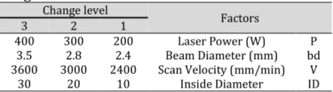
Table 1 shows the factors and their variation levels which were assumed for the design of the experiments of the laser forming of the sheet metal's hole edge.

Table 1: The effective factors in the laser forming process and the changes of level in the Taguchi method Factors Change level 1 2 3 P Laser Power (W) 200 300 400 bd Beam Diameter (mm) 2.4 2.8 3.5 V Scan Velocity (mm/min) 2400 3000 3600 ID Inside Diameter 10 20 30

To select the appropriate array, the required degrees of freedom should be calculated. According to the Table 1, each of the four factors (P, bd, V and ID) should be studied in three levels. Therefore the degree of freedom for each of the parameters was 2. The total degree of freedom for the four factors was 8 (4x2=8). The Taguchi orthogonal array should not have a degree of freedom which is less than the total

degree of freedom of the experiment. The best choice was the L9 suggested array from the array group of the Taguchi group.

According to the L9 array, the final result of the design of the experiments is presented in Table 2. Note that the number of the laser scan passes in all of the 9 experiments was 5.

Table 2: Experiment design of simulation of laser forming of hole edge by L9 orthogonal array Experiment Number P V bD ID 1 200 2400 2.4 10 2 200 3000 2.8 20 3 200 3600 3.5 30 4 300 2400 2.8 30 5 300 3000 3.5 10 6 300 3600 2.4 20 7 400 2400 3.5 20 8 400 3000 2.4 30 9 400 3600 2.8 10

For each of the circular radii scan sketches in Table 3, 9 finite element experiments in two steps (thermal step and mechanical step) were simulated according to Table 2. All of the output parameters which were important in the final collar production process design were derived (i.e. the maximum produced temperature on the sheet metal, the produced collar edge deflection and the location deflection of each of the circular scan paths on the sheet metal).

Table 3: Different combinations of radius scanning Four Radial Combined Strategy Three Radial Combined Strategy Two Radial Combined Strategy Single Radial Strategy 1,2,3,4 1,2,3 1,2 1 1,2,4 1,3 2 1,3,4 1,4 3 2,3,4 2,3 4 2,4 3,4

2.2. Finite element modeling

In the currentstudy, simulation of laser forming process has been conducted by a decoupled transient thermal–structural analysis. Abaqus Finite Element Modeling software has been employed during numerical analysis and important thermal and mechanical assumptions are described in following sections.

2.3. FEM configuration

Similar mesh grid has been employed during thermal and mechanical finite element analysis. To increase the accuracy of the results considering the importance of calculation time, smaller mesh size was considered for those meshes close to scanning path. Figure 2 shows

the distribution of mesh density around the scan path.

Figure 2: schematic of mesh density

The first order elements take shorter computation time in the first phase of mechanical analysis i.e. during determining the bending deformation. Meanwhile analysis of these elements, shear locking and hourglass effect was occurred. To obviate this problem, higher order elements, such as C3D20R twenty-node was implemented which could also affect the computation time. Consequently DC3D20 twenty-node element was employed in the heat transfer analysis to keep compatibility with the structural analysis.

2.4. FEM assumptions

In order to decrease the complexity of numerical simulation, the following simplifications and assumptions were proposed during the thermal and mechanical analyses (Yanjin et al., 2003; Liu

et al., 2008).

1. Laser intensity follows the Gaussian distribution.

2. The laser operates in continuous wave (CW) mode.

3. Solution initiates with thermal analysis, and result is then used as the initial condition for determining deformation.

4. No melting occurs during the forming process, and no external forces are applied on sheets.

5. All specimens are made of AISI 1010 (Fan et al., 2007).

6. All Thermal and mechanical properties of material including thermal conductivity, specific heat, thermal expansion coefficient, density, yield stress, Poisson’s ratio and Young’s modulus are temperature-dependent.

7. Strain rate enhancement is safelyneglected. 8. Dissipation of energy due to plastic

deformation and phase changes can be neglected comparingwith laser beam energy involved during the thermal phase.

9. The material is assumed to behomogeneous, isotropic and Von Misses theory is used as the failure criterion in the finite element simulation.

10.The sheet metal is initially stress and strain-free.

11.Isotropic hardening rule is applied by considering a linear stress strain behavior from room temperature (20o_{C) to melting} temperatures (1500o_{C)(Safdara et al., 2007).} 12.The outer edge of sheet metal is completely

fixed and there is no boundary condition on the inside edge.

13. Heat conduction in the sheet metal and free convection to the atmosphere are considered in the analysis while neglecting thermal radiation.

2.5. Setup of experiments

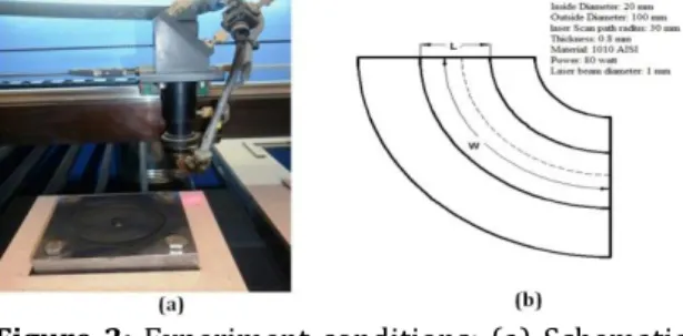
The sheet metal used for the experiments are AISI1010 with 0.8mm thickness (Figure 3-a). The outer and inner diameters were assumed to be 100 and 20 mm, respectively. To enhance the specimens' laser absorption, graphite coating has been applied to the subjected surface. The specimens have been irradiated using a 300 W output power CO2-laser. A two-axis computer numerical control (CNC) table has been utilized to control laser head (Figure 3-a). To simplify the process, the laser scan velocity, radius of concentric heating paths(R), laser power, and laser beam diameter have been adjusted to 720 mm/min, 30 mm, 80 watt and 1 mm respectively (Figure 3-b).

Figure 3: Experiment conditions: (a) Schematic of laser CNC (b) Variable setup

We conducted a set of 5 experiments with specified conditions and number of laser scan of 1 to 5. The deflection of the plate is the target in each experiment. These data are used further in verification of FEM results.

2.6. FEM verification

To verify the deformation behavior of FEA, a model with constant process parameters and various number of laser scan has been established to predict deflection. The specification of FE model has been listed in Figure 3 and Table 4.

Table 4: mesh specifications of FE models Number of elements in ring Number of elements in the outer ring Number of elements in the inner ring Number of elements in the middle ring Element shape Geometric order Element Type Band length 70 8 8 6 Hex Quadratic Standard 4 mm

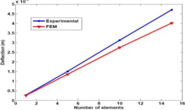
Figure 4 shows both numerical simulation and experimental results of irradiated specimen. The deflection of numerical analysis and experimental results are compared in Figure 5.

Figure 4: Experimental and numerical part of laser forming.

As illustrated in Figure 5, the deflection achieved from experiment indicated a good agreement with the finite element model, especially in low number of scans. As the number of scans increases, the result of FEA estimates less deflection comparing with experiments and the deviation of the results between two methods increases. Table 5 shows this error for different number of scans.

Figure 5: Effect of number of scans on edge deflection from FE and experimental tests The differences between numerical and experimental results are most probably because of: 1) material properties, 2) real absorption coefficient and 3) the accuracy of experimental results. Furthermore, the effect of isotropic

hardening factor is also considerable in producing the errors_.

Table 5: The edge deflections result from various numbers of scans

Number of scans Experimental results FEA results Error (%) 1 0.00028 0.00026 6.70 5 0.00151 0.00136 9.63 10 0.00313 0.00275 12.28 15 0.00471 0.00402 14.64

2.7. The Estimator Models

In this section, the results of the different algorithms which were employed for estimation of the deflection are presented. The results of these algorithms were compared with each other and finally, the results achieved from the best model were compared with the simulation and experimental results. The categorization of the models is depicted in Figure 6.

Figure 6: Classification studied estimator models.

2.8. The linear models

As mentioned in previous sections, a number of experiments were designed to study the effect of the different parameters on the deflection, and they were simulated with the ABAQUS software. The resulted data were collected afterward and employed for deflection modeling as a group of data. This group contained 192 samples, 9 input and 5 output characteristics, which are presented in Table 6.

Table 6:The relevant of variable range of values definition Variable symbol [200 400] Radiation power P Input variables [40 60] Ray speed V [2.4 3.5] Beam Diameter bd [10 30] Hole Diameter ID [0 17] The first Radius

R1

[0 19] The second Radius

R2

[0 21] The third Radius

R3

[0 23] The radius of the fourth

R4 [1 5] Number of Scan NS Edge Deflection DE

Output variables D1 D2 Deflection in second RadiusDeflection in first Radius Deflection in third Radius D3

Deflection in fourth Radius D4

To model the output parameters using the two methods, the tests were carried out according to Figure 6. Firstly the model with the assumption of the independency of the deflection in estimation and then, with the assumption of the dependency of each of the output parameters (deflection) to its previous value, called deflections dependency, are investigated. The main employed linear models are LMS (Peter et al., 1987) and M5Rule (Geoffrey Holmes and Eibe, 1999).

2.8.1. Modeling with the assumption of the independency of the deflection estimator models in different radii (deflections independency model)

The first model group is developed with the assumption of the independency of the deflection estimator models, which means that an independent model from the other models is developed from the input data for each of the output parameters (deflections).

2.8.2. The model in which the entire scan radii are integrated in one model

In this type of the models the entire single scan, double scan and multiple scan conditions were simulated in one model. The weakness of this type of modeling was that since some of the radii were not used in some experiments, the corresponding radius would be zero in that model, and therefore in that model, an estimative model between zero and the first radius was presented.

In this type of modeling, the different available algorithms were tested and their results were studied, which is presented as follows.

Table 7 shows the regression model of the best model in this category. Also the mean absolute error of this formula on the data is presented in the table. The least deflection modeling error between LMS, M5Rule, SMOReg and REPTree belonged to the LMS algorithm, which is presented in Table 7.

Table 7: sample linear estimator model with independent deflection assume for all scan radius Absolute mean

error Obtained regression formula

Used algorithm

6.980E-5 (0.00005*Power -0.0009*speed +0.006*beam diameter -0.022*Hole

Diameter-0.0032*R1+0.002*R2+ 0.0028*R3+0.0025*R4+ 0.0274*Number Scan+1.01) *(0.0011)+0.000067 LMS Edge deflection 6.54E-5 (-0.00041*Power+0.0016*speed+ 0.0325*beamdiameter-0.0203*Hole Diameter-0.0084*R1-0.0052*R2-0.0011*R3+0.0013*R-0.0019*Number of scan+0.9829)*(0.000879)-0.000023 LMS Deflection of first radius 6.39 E-5 (-0.005*Power+0.02439*speed+0.45*beam diameter-0.1823*Hole Diameter -0.0538*R1 -0.0715*R2-0.033*R3+0.00899*R4-0.1584* NumScan +7.16889)/10000 LMS Deflection of second radius 5.77 E -5 (-0.048*Power+0.24*speed+4.3*beam diameter+-1.8*Hole

Diameter-0.131*R1-0.46*R2-0.48*R3-0.114*R4-1.9* NumScan +62.8)/10000 LMS

Deflection of third radius

5.63 E-5 (-0.027*Power+0.068*speed+5.9*beam diameter-1.7*Hole

Diameter-0.089*R1-0.3309*R2-0.3452*R3-0.2171*R4-1.5086* NumScan +53.7602)/10000

LMS Deflection of

fourth radius

2.8.3. Linear Modeling of separation of the RADIUS

Regarding the previous model weakness about the existence of the zero radii in the model, a new model was proposed that its category was determined using the number of the data scans.

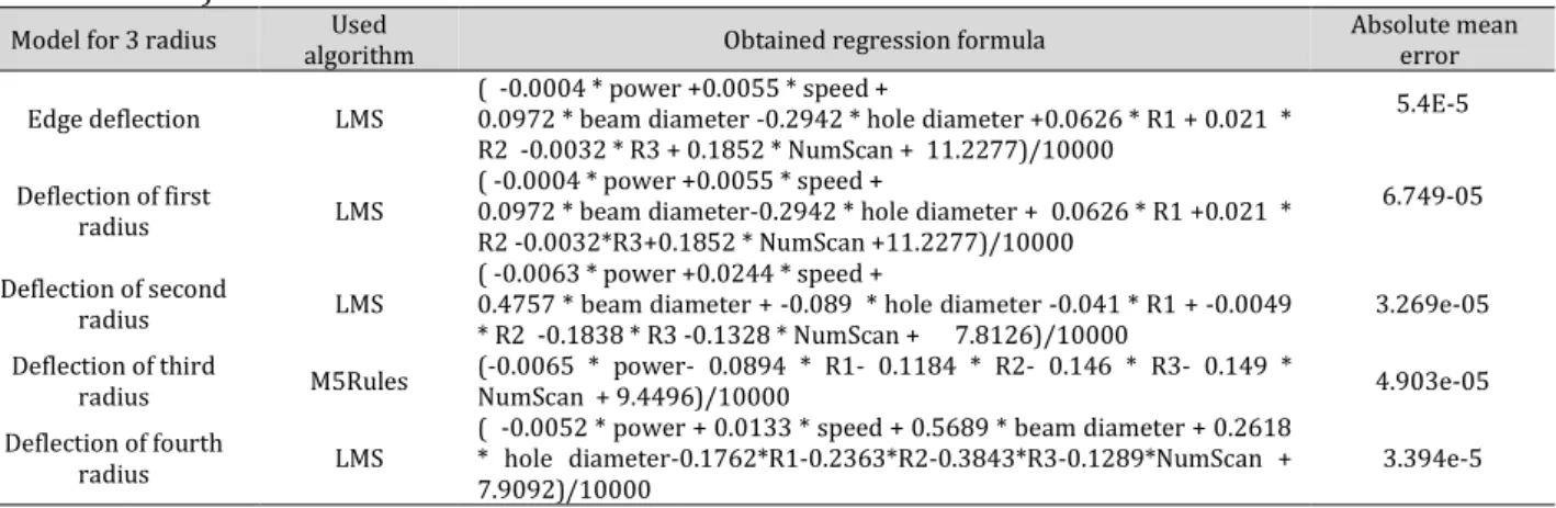
In this type of modeling three model categories was presented for the data which were adopted for single radial, double radial and triple radial estimates (Table 8). Generally, the mean error value of this model was less than that of the other models.

Table 8: estimator model with independent deflection assume for any scan radius (only presented model with 3 radius)

Absolute mean error Obtained regression formula

Used algorithm Model for 3 radius

5.4E-5 ( -0.0004 * power +0.0055 * speed +

0.0972 * beam diameter -0.2942 * hole diameter +0.0626 * R1 + 0.021 * R2 -0.0032 * R3 + 0.1852 * NumScan + 11.2277)/10000

LMS Edge deflection

6.749-05 ( -0.0004 * power +0.0055 * speed +

0.0972 * beam diameter-0.2942 * hole diameter + 0.0626 * R1 +0.021 * R2 -0.0032*R3+0.1852 * NumScan +11.2277)/10000 LMS Deflection of first radius 3.269e-05 ( -0.0063 * power +0.0244 * speed +

0.4757 * beam diameter + -0.089 * hole diameter -0.041 * R1 + -0.0049 * R2 -0.1838 * R3 -0.1328 * NumScan + 7.8126)/10000 LMS Deflection of second radius 4.903e-05 (-0.0065 * power- 0.0894 * R1- 0.1184 * R2- 0.146 * R3- 0.149 * NumScan + 9.4496)/10000 M5Rules Deflection of third radius 3.394e-5 ( -0.0052 * power + 0.0133 * speed + 0.5689 * beam diameter + 0.2618

* hole diameter-0.1762*R1-0.2363*R2-0.3843*R3-0.1289*NumScan + 7.9092)/10000

LMS Deflection of fourth

radius

2.8.4. Modeling with the assumption of the dependency of the deflections to each other The modeling with the assumption of the deflections independency was carried out and presented in previous sections. However, regarding the high amount of correlativity of the different deflections, it was necessary to assume that they were relative and therefore for the final conclusion, this condition should also be modeled. The assumed relativity graph for modeling is presented in Figure 7. In this model the parameters DE, D1, D2, D3 and D4 are the collar edge deflection, the first radial location deflection, the second radial location deflection, the third radial location deflection and the forth radial location deflection respectively. In this condition the edge deflection was just the function of the input parameters, but the other parameters were the functions of the previous deflections in addition to the input parameters.

Table 9 shows the regression formula of each of the models in which the correlativity of the models in the modeling procedure is taken into account. These formulas were derived after the normalizing the data.

Figure 7: Intended for dependency graph modeling.

Table 9: sample estimator model with dependent deflection assume

Absolute mean error Obtained regression formula

Used algorithm 7.97 E-5 0.0074*Power-0.0117*SPEED-0.0061*bd-0.4358*HOLE-DIAMETER-0.0409*R1+0.0177*R2 +0.0368*R3+0.0399*R4+0.0937*I+0.8178 LMS DE

The deflection estimation errors in the deflections' dependency and independency conditions are illustrated in Figure 8. As it can be seen in the Figure 8, in the first condition the estimated error was lower, note that the data were normalized. On the other hand, by regarding additional deflections in the formula in the correlativity of the deflections condition, the estimated error was increased.

According to the achieved results it was concluded that the calculations with correlativity assumptions in the estimator models between the parameters did not lead to good results, while development of the independent models led to more accurate

results. The main reason of such a result is the error accumulation in the parameters.

Figure 8: Comparison of estimates of the error in a State of independent and depended of deflection

2.9. Non-linear models

The non-linear models which are extensively applied for complex systems are: neural network, genetic algorithm, genetic programming, non-linear regression etc. among these models, three models out of the most famous neural network and genetic programming models were used. The results are presented in Figure 9 and Table 11.

RESULTS

3.1. The results of the genetic programming Table 10 shows the required equations for edge deflections estimation and other radial locations. These formulas were developed after the normalization of the data. In this table the parameters DE, D1, D2, D3 and D4 are the collar edge deflection, the first radial location deflection, the second radial location deflection, the third radial location deflection and the forth radial location deflection respectively.

Table 10: sample of non-linear dependent estimator models with the help of (GP)

mean Absolute error

Obtained regression formula

7.87e-5 (((num scan/(3.8+num scan))+hole diameter)/(((speed*hole diameter)*((7.9/speed)*((hole

diameter+(((r2/(beam diameter*((7.9+3.8)+(3.8-\r3))))+7.9)+(hole diameter-(speed/beam diameter))))+speed)))+((((num scan/((((hole diameter+(7.9+(hole diameter-(speed/beam diameter))))-hole diameter)*(3.8+(hole diameter-(speed/hole diameter))))-hole diameter))+hole diameter)*((7.9*(hole diameter+(7.9+3.8)))+((3.8-hole diameter)*(((hole

diameter-(speed/3.8))*(r1/(((r3/(((7.9/7.9)/num scan)-(7.9/speed)))/hole diameter)-(((7.9+(r3/(3.8+num scan)))-(r1/3.8))*(speed/3.8)))))+num scan))))*3.8)))

DE

3.2. The results of the neural network models For modeling with the neural network algorithm three common networks were employed namely Perceptron, Feed forward back propagation and Radial basis. Their results were presented in Table 11. It was shown that the results of back propagation network, which is in fact a multi-layer Perceptron network, was better than the other neural network models.

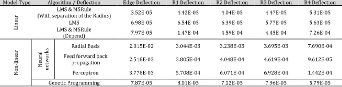
3.3. Comparison between the accuracy of the linear and non-linear models

In the following figure (Figure 9) the test mean absolute error values of the linear and non-linear tested models in all the conditions are compared.

Figure 9: Comparing the accuracy of linear and non-linear models

According to the Figure 8 and Figure 9, it is obvious that the amount of the error in linear models is significantly lower than that in non-linear models. The dependent models' errors are also more than that of the linear models.

Table 11: The results of the error values for all models

R4 Deflection R3 Deflection R2 Deflection R1 Deflection Edge Deflection Algorithm / Deflection Model Type 5.31E-05 4.47E-05 4.04E-05 4.42E-05 3.52E-05 LMS & M5Rule

(With separation of the Radius)

Lin ea r 5.63E-05 5.77E-05 6.39E-05 6.54E-05 6.98E-05 LMS 7.26E-04 4.45E-04 4.59E-04 1.47E-04 7.97E-05 LMS & M5Rule (Depend) 7.690E-04 3.695E-03 3.238E-03 3.044E-03 2.015E-02 Radial Basis Ne ur al ne tw or ks No n-line ar 9.612E-05 4.619E-04 4.048E-04 3.805E-04 2.518E-03 Feed forward back

propagation 1.442E-04 6.928E-04 6.071E-04 5.708E-04 3.778E-03 Perceptron 5.79E-05 7.96E-05 7.12E-05 8.01E-05 7.87E-05 Genetic Programming

One of the main reasons of such results was the number of the input data used for modeling. Since the non-linear models are more complex and have more parameters, that finding the optimized amount of each of these parameters demands that more available data. Hence, usually in nonlinear models a large amount of data is needed for system training. On the other hand, in machine learning field the over fitting phenomenon should be considered, which states

that when a model is adapted too much with the training data, generally it has poor predictive performance. As a result, the amount of error of the test data would increase. Hence the simpler the model, the more general it would be (Peter

et al., 1987; Geoffrey Holmes and Eibe, 1999).

Since the linear models are among the simplest models, they have high ability of generalization. Therefore the comparison between the different model results which are presented in Table 7 to

Table 11 shows that the most appropriate model for deflection estimation was the model which is presented in Table 8 (the linear estimator model with the assumption of deflection independency for each of the scan radii). It can be observed that the amount of the error value in this model was lower than the other models.

DISCUSSION AND CONCLUSION In this research the different linear and nonlinear estimator models were employed in laser forming process of the circular paths to reduce the estimation time. The study of these models revealed that regarding the limitation of the number of the input data experiments which were obtained from finite element simulation and experimental tests, the best applicable model was the linear model. The reason is that firstly the estimator model of each of the radii was independent from the other radii and secondly, according to the number of required scans, the corresponding single radial, double radial or triple radial model was employed. Note that these limitations normally exist in application. The results showed that among the estimator models, the error value in models in which the deflection in each radius is dependent to the amount of deflection in the smaller radius was more than that in models in which the deflection in each radius is derived directly from the existing data. According to the results, the mean error value between the dependent condition and the selected condition was about 80%. Also the results showed that the results of the linear models were higher than the nonlinear models. According to the results, the error value between all of the tested nonlinear conditions and the best selected condition was about 76.9%.

REFERENCES

Chen DJ, Xiang YB, et al. Application of fuzzy neural network to laser bending process of sheet metal. Materials science and technology 2002;18(6):677-680.

Cheng JG, Yao YL. Process synthesis of laser forming by genetic algorithm. International Journal of Machine Tools and Manufacture 2004;44(15):1619-1628.

Cheng P, Lin S. Using neural networks to predict bending angle of sheet metal formed by laser. International Journal of Machine Tools and Manufacture 2000;40(8):1185-1197.

Fan Y, Yang Z, et al. Investigation of Effect of Phase Transformations on Mechanical Behavior of AISI 1010 Steel in Laser Forming. Journal Of Manufacturing Science And Engineering 2007;129:110-116.

Geiger M, Vollertsen F, et al. Flexible straightening of car body shells by laser forming. International Congress and Exposition 1993.

Geiger M, Arnet H, et al. Laser forming. Manufacturing Systems 1995;1:43-47. Geoffrey Holmes MH, Eibe F. Generating Rule

Sets from Model Trees. Conference on Artificial Intelligence, Australia 1999.

Hoseinpour Gollo M, Mahdavian S, et al. Statistical analysis of parameter effects on bending angle in laser forming process by pulsed Nd: YAG laser. Optics & Laser Technology 2011;43(3):475-482.

Khani DM. introducing with design for experiment and taguchi method. Zanjan University Publisher, 2006. [In Persian] Liu FR, Chan KC, et al. Numerical modeling of the

thermo-mechanical behavior of particle reinforced metal matrix composites in laser forming by using a multi-particle cell model. Composites Science and Technology 2008; 68:1943–1953.

Mahdi Asadollah SIG. Functional Laser Forming Optimization of a Metal Strip. Master Of Science (MSc), University of Kashan 2013. [In Persian]

Maji K, Pratihar DK, et al. Analysis and synthesis of laser forming process using neural networks and neuro-fuzzy inference system. Soft Computing 2013;pp:1-17.

Peter J. Rousseeuw AML. Robust regression and outlier detection, 1987.

Safdara S, Lia L, et al. Finite element simulation of laser tube bending: Effect of scanning schemes on bending angle, distortions and stress distribution. Optics & Laser Technology 2007;39:1101-1110.

Scully K. Laser line heating. Ship Production Symposium 1900.

Shekhar Chakraborty S, Racherla V, et al. Parametric study on bending and thickening in laser forming of a bowl shaped surface. Optics and Lasers in Engineering 2012. Shi Y, Yao Z, et al. Research on the mechanisms

of laser forming for the metal plate. International Journal of Machine Tools & Manufacture 2006;46:1689–1697.

Shimizu H. A heating process algorithm for metal forming by a moving heat source, Massachusetts Institute of Technology 1997. Yanjin G, Sheng S, et al. Finite element modeling

of laser bending of pre-loaded sheet metals. Journal of Materials Processing Technology 2003;142(2):400-407.

Yau C, Chan K, et al. Laser bending of leadframe materials. Journal of Materials Processing Technology 1998;82(1):117-121.