Modeling of Spontaneous Activity in Developing Spinal Cord Using
Activity-Dependent Depression in an Excitatory Network
Joe¨l Tabak,
1Walter Senn,
2Michael J. O’Donovan,
1and John Rinzel
31
Laboratory of Neural Control, National Institute of Neurological Diseases and Stroke/National Institutes of Health,
Bethesda, Maryland 20892,
2Physiologisches Institut, Universita¨t Bern, CH-3012 Bern, Switzerland, and
3Center for
Neural Science and Courant Institute of Mathematical Sciences, New York University, New York, New York 10003
Spontaneous episodic activity is a general feature of develop-ing neural networks. In the chick spinal cord, the activity com-prises episodes of rhythmic discharge (duration 5–90 sec; cycle rate 0.1–2 Hz) that recur every 2–30 min. The activity does not depend on specialized connectivity or intrinsic bursting neu-rons and is generated by a network of functionally excitatory connections. Here, we develop an idealized, qualitative model of a homogeneous, excitatory recurrent network that could account for the multiple time-scale spontaneous activity in the embryonic chick spinal cord. We show that cycling can arise
from the interplay between excitatory connectivity and fast synaptic depression. The slow episodic behavior is attributable to a slow activity-dependent network depression that is mod-eled either as a modulation of cellular excitability or as synaptic depression. Although the two descriptions share many fea-tures, the model with a slow synaptic depression accounts better for the experimental observations during blockade of excitatory synapses.
Key words: spontaneous activity; oscillations; depression; developing spinal network; recurrent excitation; rate model
Spontaneous activity generated by networks of synaptic connec-tions is a characteristic, but poorly understood, feature of the developing nervous system. It has been detected in many different regions, including the retina, the hippocampus, and the spinal cord. In each region, bouts of activity occur episodically, sepa-rated by periods of quiescence. Although the mechanisms respon-sible for this activity are incompletely understood, it is known that developing networks are hyperexcitable, in part, because the classically inhibitory neurotransmitters, GABA and glycine, are depolarizing (Cherubini et al., 1991; Sernagor et al., 1995).
We have been studying this activity in the isolated lumbosacral spinal cord of the chick embryo. This preparation generates spontaneous episodes of activity in which spinal neurons are cyclically activated (see Fig. 1). This activity is not produced at a specific location, nor by a specific set of connexions (Ho and O’Donovan, 1993), and is still present in networks for which glutamatergic transmission or glycinergic/GABAergic transmis-sion has been blocked (Chub and O’Donovan, 1998a). It has also been shown that episodes of activity transiently depress network excitability, which recovers in the quiescent phase; this depression is manifest as decreased synaptic strength (Fedirchuk et al., 1999) and hyperpolarization of individual cells. These observations have led to the proposal that the occurrence of episodes is a population phenomenon that is controlled by activity-dependent network depression (O’Donovan and Chub, 1997; O’Donovan, 1999). There is evidence that spontaneous bursts or episodes in
other parts of the nervous system are also regulated by a form of activity-dependent depression. A slow “refractoriness” is thought to restrict wave generation and propagation in the newborn ferret retina (Feller et al., 1996, 1997; Butts et al., 1999). In hippocampal networks, NMDA receptor desensitization (Traub et al., 1994) or presynaptic depletion of glutamate pools (Staley et al., 1998) have been proposed to regulate the occurrence and/or duration of synchronous bursts.
Less is understood about the mechanism of cycling within an episode, but it has been proposed that this could also be regulated by activity-dependent depression with much faster kinetics than the depression controlling episodes [O’Donovan and Chub (1997); see also Streit (1993)]. Recently, it has been shown in modeling studies that a purely excitatory network with random connections susceptible to fast depression is capable of generating oscillations similar to the cycling observed during episodes (Senn et al., 1996; J. Streit and W. Senn, unpublished results).
Using these ideas, we develop a simple and general model of network activity. This model describes only the average firing rate of the population, rather than the membrane potential and spikes of the individual neurons. It assumes a purely excitatory recurrent network that is susceptible to both short- and long-term activity-dependent depression (see Fig. 2A). The model is de-scribed by only three coupled nonlinear differential equations. Therefore, the analysis can be done graphically, step by step, which facilitates an intuitive understanding of the network dynamics.
We show that this simple model can account for the occurrence of spontaneous episodes, the rhythmic cycling within an episode, and the developmental changes in the duration of episodes and interepisode intervals. Most importantly, it shows that the recov-ery of spontaneous activity in the presence of excitatory amino acid blockers (Barry and O’Donovan 1987; Chub and O’Donovan 1998a) is a property of networks with a slow form of synaptic depression.
Received Aug. 31, 1999; revised Jan. 1, 2000; accepted Jan. 10, 2000.
J.R. acknowledges the support and hospitality of the Mathematical Research Branch, National Institute of Diabetes and Digestive and Kidney Diseases, and the Laboratory of Neural Control, National Institute of Neurological Diseases and Stroke, which facilitated his participation in this research. We thank Uri Cohen for comments on a previous version of this manuscript.
Correspondence should be addressed to Joel Tabak, Laboratory of Neural Con-trol, Room 3A50, Building 49, National Institutes of Health, Bethesda, MD 20892. E-mail: [email protected].
Parts of this work have been presented previously in abstract form (Rinzel and O’Donovan, 1997) and conference proceedings (O’Donovan et al., 1998; Tabak et al., 1999).
MATERIALS AND METHODS Experimental
All experiments were performed on the isolated spinal cord of White Leghorn chicken embryos maintained in a forced-draught incubator. The spinal cord was dissected out under cooled (12–15°C) oxygenated (95% O2, 5% CO2) Tyrode’s solution containing (in mM): 139 NaCl, 12 glucose, 17 NaHCO3, 2.9 KCl, 1 MgCl2, 3 CaCl2. The preparation was transferred to a recording chamber (at room temperature) and super-fused with oxygenated Tyrode’s solution that was later heated to 26 – 28°C. The concentration of KCl was raised to 5– 8 mMduring some of the
recordings to accelerate the recovery of activity after glutamatergic blockade (Chub and O’Donovan, 1998a).
Neural activity was recorded from ventral roots or muscle nerves. Recordings were made using tight-fitting suction electrodes and ampli-fied (DC 3 kHz) with high gain DC amplifiers (DAM 50 and IsoDAM, World Precision Instruments). Amplified signals were directly digitized through a PCI board (National Instruments) and/or recorded on tape (Neurodata) for further analysis. Recordings were digitized at a low sampling rate (5–20 Hz) because the events of interest occur on a slow time scale (Fig. 1).
Theoretical
Model equations.The two models are described and analyzed in depth in Results. Here we present them and the associated parameter values more succinctly. Both models have three dynamical variables, includingaand d: a is the population activity or mean firing rate, and d is the fast depression variable, representing the fraction of synapses not affected by
the fast synaptic depression. These two variables generate the cycles within an episode. The slow modulation that underlies onset and termi-nation of episodes, and the long silent phases, is described byors. represents the threshold for cell firing. In the-model, it increases slowly during an episode, eventually terminating the episode and recovering between episodes. In thes-model,srepresents the fraction of synapses not affected by the slow synaptic depression, decreasing slowly during an episode, terminating it, and then recovering between episodes. In the s-model, the fraction of nondepressed synapses at any given time is therefore the products䡠d.
The equations for the models are: -model: aa˙⫽a⬁共n䡠d䡠a兲⫺a, (1) dd˙⫽d⬁共a兲⫺d, (2) ˙⫽⬁共a兲⫺, (3) s-model: aa˙⫽a⬁共n䡠s䡠d䡠a兲⫺a, (4) dd˙⫽d⬁共a兲⫺d, (5) ss˙⫽s⬁共a兲⫺s. (6)
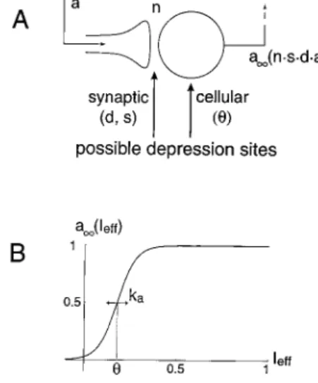
The parameter n measures the connectivity in the network (see Results). All of thex⬁functions are sigmoidal (e.g., see Fig. 2Cfor a plot ofa⬁):
a⬁共Ieff兲⫽1Ⲑ共1⫹e⫺共Ieff⫺兲/ka兲 d⬁共a兲⫽1Ⲑ共1⫹e共a⫺d兲/kd兲
⬁共a兲⫽1Ⲑ共1⫹e⫺共a⫺兲/k兲 s⬁共a兲⫽1Ⲑ共1⫹e共a⫺s兲/ks兲.
The parameterxdefines the argument’s value for which half-activation occurs:x⬁(x)⫽1/2. The value ofkx(positive) determines the sigmoid’s steepness, smaller values being steeper. Note that the presence (respec-tively absence) of a minus sign in front of (a⫺x) indicates that the sigmoid is increasing (respectively decreasing). The variablesdandsare high for low activity (low depression) and low for high activity (high depression), sod⬁(a) ands⬁(a) are decreasing functions ofa.
Althougha⬁is the cellular input–output function, it should be con-sidered as an average over the population of neurons. Assuming these neurons are not identical,a⬁inherits a sigmoid shape;can be inter-preted as the mean threshold andkaas the threshold variance, assuming a unimodal distribution of thresholds (Wilson and Cowan, 1972). Be-cause the connectivity coefficients are included inside thea⬁function,a should be interpreted as mean population firing rate averaged over a brief period of time, not as instantaneous voltage (Pinto et al., 1996); a⬁(n䡠s䡠d䡠a) is the instantaneous firing rate. Note that becausea⬁(0) is not equal to zero, we are implicitly assuming that there is some background activity or fraction of spontaneously active neurons in the network. However, the model does not depend on this feature. Indeed, ifa⬁(0)⫽ 0, similar episodes of activity are produced, except thatastays virtually at 0 from just after an episode to just before the next one (our unpub-lished results).
Unless stated otherwise, we use the parameter values given in Table 1. Simulations.The model equations were implemented within XPPAUT (freely available software by G. B. Ermentrout, http://www.pitt.edu/ ⬃phase/), a general purpose interactive package for numerically solving and analyzing differential equations. XPPAUT includes a tool for calcu-lation of bifurcation diagrams (AUTO). Simucalcu-lations were performed using the Runge–Kutta integration method with a time step of 0.2 (dimensionless units). We checked that the results were unchanged when the time step was halved. Simulations were run on Unix PCs. A version of the software WinPP runs under Win95 or Win98.
RESULTS
We have argued elsewhere (Ritter et al., 1999) that the spinal network responsible for spontaneous activity is composed of
Figure 1. Spontaneous episodes of activity recorded from ventral roots of chick embryo spinal cordin vitroat embryonic day (E) 7.5 and 10. Recordings were made in DC mode and digitized at 10 Hz, showing the synaptic depolarization recorded electrotonically from motoneurons. Pe-riods of activity (episodes) are clearly distinct from silent phases. An interval is defined as the time between the beginning of two consecutives episodes. Episodes are composed of cycles, or “network spikes.” With development, both the interval and episode duration lengthen, and cycle frequency and the level of depolarization (tonic component) also in-crease. Also, on older embryos episodes have a leading tonic phase before cycling begins. For the examples shown here, interval and episode dura-tions are, respectively, E 7.5: 440⫾29 and 20⫾1 sec; E 10: 1600⫾140 and 68⫾3.5 sec (mean⫾SD).
recurrently connected, functionally excitatory synaptic connec-tions. Furthermore, because the expression of network activity does not appear to depend on the details of network architecture or membrane properties and because detailed biophysical infor-mation on cell and coupling properties is unavailable, we are justified in using a very idealized model. Throughout, we use mean field models that describe only the averaged population behavior, not the detailed electrical activity of individual cells. The models are also temporally coarse-grained so that action potentials are not represented per se, only firing rate.
Our graphical analysis of the models proceeds by considering reduced models, beginning with the fastest process first and expanding the model by stepwise introduction of the next slower variables. We begin with the single Equation 1 that governs the dynamics of a recurrent excitatory network, without the negative feedback of depression. This reduced model illustrates the clas-sical behavior of bistability in a recurrent population, of either a low or high activity state of steady firing. Next, we introduce a fast activity-dependent synaptic depression, which can lead to net-work oscillations (cycling) in this two-variable system. We ana-lyze this subsystem with phase plane methods, finding a different type of bistability. Finally, we add slow activity-dependent de-pression in either of two forms and show that these three-variable models can generate episodes similar to those observed experi-mentally in the chick embryo spinal cord and other networks. A recurrent excitatory network can be bistable
In this section, we consider only the dynamics of the average activity in a random excitatory network; the depression variables are frozen. We use a graphical method to illustrate how the steady activity states of the one-variable system are determined. These steady states depend on parameters such as the network connec-tivity, and we show that for certain values of connectivity the network can have two stable states.
Here, and throughout, we letabe a measure of the network activity, for instance the population’s mean firing rate, relative to the maximum possible rate. Its time behavior, according to clas-sical descriptions (Wilson and Cowan, 1972), satisfies a a˙ ⫽ a⬁(Ieff) ⫺a, where a˙is the time derivative of a and Ieffis the
effective input to cells in the network. Accordingly, the activity of the network reaches the valuea⬁(Ieff) with a time constanta.a⬁
is called the activation function and describes how Ieff is con-verted into firing rate (Fig. 2B). For small inputs,a⬁is near 0;
very few neurons are firing. For large inputs,a⬁saturates at 1,
with all cells in the network being fully active. There is a rather sharp transition between these two limits (ifkais small) at the valueIeff⫽for whicha⬁()⫽1⁄2.corresponds to the average
threshold for cell firing. The mathematical expression of a⬁ is
given in Materials and Methods.
Because of the recurrent connectivity, the inputIeffis produced by the network’s own activity, in addition to any external inputs. Therefore, in the absence of external inputsIeff⫽n䡠a, where we introduce the parameternas a measure of network connectivity (in arbitrary units). The greater the connectivity, the greater the recurrent input being fed back to the network for a given amount of activity (n is a gain parameter, measuring how the average cellular output is transmitted to other cells, and thus depends on many physiological parameters such as the average number of contacts from a neuron, average synaptic efficacy, etc.). Thus, the dynamics of this network is described by:
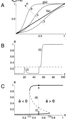
aa˙⫽a⬁共n䡠a兲⫺a. (1⬘) What is the behavior of the system defined by Equation 1⬘? After any transient input,awill evolve to a steady state, for which a˙⫽0. Its value at steady state must then satisfya⫽a⬁(n䡠a). The
solutions to this equation are represented graphically in Figure 3Aas the intersections of the curvesf(a)⫽aandg(a)⫽a⬁(n䡠a)
for different values ofn.
For small values ofn, there is only one steady state, at a low value of a, with the network barely active because of its low, functional connectivity. Even if the network receives a strong transient external input, it will return to this quiescent state because the connectivity is too low to sustain the activity. Simi-larly, for large connectivity, there is only one possible steady state (the curves do not actually intersect at the low level), for which Table 1. Values of the parameters used for each model, unless
mentioned otherwise in text or figure
Parameter -model s-model
n 1 1 a 1 1 Variable 0.18 ka 0.05 0.05 d 2 2 d 0.2 0.5 kd 0.5 0.2 1000 0.15 k 0.05 s 500 s 0.14 ks 0.02
Figure 2. A, Schematic diagram of recurrent network with random connections. The output from the network is fed back to the cells. The amount of feedback depends on network connectivity (n). Activity (a) can also be modulated at the synaptic level by a fast depression (d) and by a slow depression (s). The effective input to cells is thereforen䡠s䡠d䡠a. The resulting postsynaptic firing rate, at steady state, is given bya⬁(a䡠d䡠s). This postsynaptic firing rate can also be modulated by the cells’ threshold (). Note, our mathematical formulation does not distinguish presynaptic and postsynaptic effects.B, Cellular input–output relationship, averaged over the population.Ieffis the effective input to the network (see Results). The
cellular threshold parametercan also be viewed as a slowly modulated variable.kameasures the width of the transition range around threshold;
the network is very active (a near 1). A more interesting case occurs for intermediate values of the connectivity parameter: there are three steady states, at low, intermediate, and high values ofa. However, the intermediate steady state isunstable. That is, a small perturbation from it will grow, and the network activity will evolve toward one of the two other steady states. Therefore, the network has two possible stable steady states; it isbistable. If the network is in the low steady state, it can be switched to the high steady state by a transient stimulus that bringsaabove the intermediate steady state, which is the effective network old. If the stimulation does not increase the activity above thresh-old, the network will fall back to low activity after the stimulus. This network threshold is not equal to the cell threshold; for example, ifa⬁is very steep, the network threshold approximately
equals/n; it decreases with increasing connectivity. Note that once the network has switched from the low to high (or high to
low) state, it will stay in the new state even though the perturba-tion has stopped. It will not return to the previous state, unless a new perturbation of sufficient magnitude occurs (if neural noise were incorporated explicitly in the model there might be sponta-neous transitions between the two states). This type of bistable behavior, illustrated in Figure 3B(see figure legend), is charac-teristic of recurrent excitatory networks (Wilson and Cowan, 1972). In the next sections, we will find that bistability underlies our models’ episodic rhythms; slow modulation leads to transi-tions between the attracting pseudostates of cycling during an episode and quiescence between episodes.
Figure 3Csummarizes the above results by showing the activity levels at steady state (a˙⫽0) over a range of nvalues. Again, it illustrates that for low connectivity/efficacy (nsmall) there is only one steady state at low activity. For strong connectivity (nnear 1 and above) only the high activity state is present. For an inter-mediate range ofnvalues both stable states coexist, along with an unstable state of intermediate activity (dashed line). The states are continuously connected as you travel along the S-shaped curve. However, as n is varied over the range, one encounters discontinuous transitions between the stable states, at the S-curve’s knees. This figure, showing the different possible activ-ity states for all values of a control parameter, is called a bifur-cation diagram [see Strogatz (1994); a bifurbifur-cation is a point for which there is a qualitative change in the dynamics of the system, like at the knees]. It will be useful to distinguish the three “branches” of such S-curves: upper, lower, and middle. Here, upper and lower ones correspond to the stable steady states, and the middle one corresponds to the unstable steady state. The middle branch is a separatrix between the upper and lower branches: any state of the network above it (i.e., on the right side of the S-curve) will evolve toward the high steady state, and any state below it (i.e., on the left side of the diagram) will fall to the low steady state. It is easy to understand why: for any point on the S-curve, by defini-tion,a˙⫽0. If the connectivity is increased (i.e., the point shifted to the right) even slightly, this increasesa⬁(n䡠a), and thereforea˙⬎0.
Conversely, ifnis decreased this leads toa˙⬍0. A recurrent excitatory network with fast activity-dependent synaptic depression can produce oscillations
In the above section, we studied the behavior of a recurrent excitatory network as a function of its (fixed) connectivity. Here, we will analyze network behavior when the effective connectivity is changing because of synaptic depression. We will analyze the resulting two-variable system graphically in the phase plane and show that it can generate oscillations (like the cycling during an episode) and bistability, depending on the average neuronal excitability.
As a preliminary step, reconsider Figure 3Cand suppose that we sweepnslowly back and forth over a range that includes the bistable regime. This would lead to alternating phases of high and low activity, with sharp transitions between phases. If n were decreasing while the activity is high, the system’s state point would track the upper branch, moving leftward, until we reached the S-curve’s left knee. Then the state point would fall to the lower branch. The activity would drop precipitously. Now at low activity, ifn were increasing, the system would track the lower branch, with activity rising very gradually, until the right knee was reached. Then the state point would jump back to the upper branch of high activity, completing a cycle, and the process would repeat.
Figure 3. Analysis of the single-variable activity model for a recurrent excitatory network.A, The steady states satisfya⬁(n䡠a)⫺a⫽0. They are determined by the intersection(s) between the curvesf(a)⫽a(thick line) andg(a)⫽a⬁(n䡠a) (smooth curves), shown here for different values ofn. At these intersectionsa⬁(n䡠a)⫺a⫽0.B, Time course of the activity for n⫽0.5. Att⫽20 a brief stimulus is applied but fails to bring the network above threshold (i). Stronger stimulation applied att ⫽50 excites the network above threshold, so the high activity steady state is reached (ii). The network will stay at this high level unless a large perturbation brings it back below threshold.C, Plot of the steady-state values ofa for all possible values ofnbetween 0 and 1. Thedashedportion of thecurve indicates unstable steady states. InAandC, the steady states forn⫽0.5 are represented byfilled(stable) or open(unstable)circles. Thearrows indicate that the activity, if initially below threshold (unstable steady state), will fall back to the low stable state (i,a˙⬍0), and if it is initially above network threshold it will increase until it reaches the high stable state (ii,a˙⬎0), as illustrated inB.⫽0.18.
We really want a description so that such cycling happens spontaneously, rather than being driven as above. With this goal we make the effectiveconnectivity a dynamic variable by multi-plying n by the variable d, the kinetics of which depends on activity, guaranteeing thatdautomatically decreases when activ-ity is high and increases for low activactiv-ity. In this formulation,dis defined as the fraction of nondepressed synapses from a repre-sentative cell to its targets (e.g., the fraction of releasable transmit-ter at those synapses). Its value ranges from 0 (synapses totally depressed) to 1 (all synapses fully available), so the effective connectivity (n䡠d) ranges from 0 ton(n, being an arbitrary measure of connectivity can be⬎1). In all of the following figures, we set n⫽1 unless mentioned otherwise. Equation 1⬘thus becomes:
aa˙⫽a⬁共n䡠d䡠a兲⫺a. (1) This idealized model does not distinguish between gluta-matergic excitatory synapses or depolarizing gabaergic/glyciner-gic synapses.
We use a simple first-order kinetics ford, reminiscent of the gating kinetics in Hodgkin–Huxley-like models for voltage-gated ionic currents:
dd˙⫽d⬁共a兲⫺d, (2)
whered⬁(a) is a decreasing sigmoid function (see Materials and
Methods). When the system is at low activity,dtends to increase, whereas for high activityd decreases.dtends towardd⬁(a) but
lags behind changes in a with a time constant d. Hence, the system can potentially oscillate, but whether it does depends on parameter values. For example, if the negative feedback from depression is too fast, the oscillations are precluded. The condi-tion (parameter relacondi-tionship) for which oscillacondi-tions emerge in the model is given in the Appendix.
We need to examine the dynamics of thisa⫺dsystem over a range ofvalues, because in later sectionswill become a slow modulatory variable. Forsmall, the network is highly excitable, and it operates at a steady high-activity level. If the network is held at a low activity level with synapses fully available and then released (Fig. 4A), it tends to its desired high level; in this case, it shows damped oscillations around the steady state because the depression is delayed (in the same way as the “delayed rectifier” potassium current does not turn on immediately after a voltage increase).
The system’s time course from Figure 4A can be viewed in another way, as a trajectory by plotting in the (a,d) plane simul-taneously the points defined by the values ofaanddat consec-utive and equally spaced times (Fig. 4B, dotted line). Although time is not represented explicitly on such a diagram, velocity along the trajectory can be deduced from the spacing between consecutive points. Here, on release from low activity the net-work quickly (large spacing between points) moves toward a state of high activity with the synapses depressed, slowing down (small spacing between points) as it approaches the steady state, in a spiraling fashion (the damped oscillation).
Using thea⫺dplane, we can analyze and predict qualitatively the system’s dynamical behavior and the consequences of chang-ing various parameters [for an introduction to phase plane anal-ysis, see Rinzel and Ermentrout (1998) or Strogatz (1994)]. The power of this graphical/geometrical approach comes largely from understanding the two solid curves in Figure 4B. These curves are called the nullclines. Thea-nullcline is defined as the relationship betweenaanddthat is obtained by settinga˙⫽0. Similarly, the
d-nullcline comes from settingd˙⫽0. Given these nullclines, we can map out the flow directions in the phase plane, according to the different areas delimited by the nullclines. For example, in the area on the right of thea-nullcline and above thed-nullcline, we know thatamust be increasing andddecreasing (hence thearrow pointing up and left). Also, we know thatamust be at a local minimum or maximum when the trajectory crosses thea-nullcline and so on. Where the nullclines intersect, neither a nor d is changing, and this corresponds to a steady state of the system.
Thea-nullcline is defined implicitly according toa⫽a⬁(n䡠d䡠a).
For a physiological interpretation, considerdas a parameter so that points on thea-nullcline are the steady-state values ofaat which decay ofabalances the regenerative input from recurrent excitation in Equation 1. Of course, the result is similar to the S-curve in Figure 3C. Thed-nullcline is simply the graph ofd⬁(a).
The nullclines are drawn in Figure 4B, showing that there is only one possible steady state (the unique intersection of the two curves). In general there can be one or three (exceptionally two) intersections, as we will show below for some values of . The a-nullcline has the characteristic switchback form (S-shape) of autocatalysis in nonlinear excitable and oscillatory systems. Al-though the steady state is stable in this case, it could be made unstable by increasingdto slow the negative feedback process, in which case the activity would become oscillatory.
For sufficiently large values of, there is again only one steady state, but now at a low activity level: in Figure 5B, the unique intersection of the nullclines near the abscissa at d ⫽ 0.923 (vertical arrow). Note that thea-nullcline’s low-activity branch is very close to the abscissa. This network model isexcitable. If the system is stimulated briefly but adequately while at this quiescent,
Figure 4. Dynamical behavior of thea⫺dsystem for low firing thresh-old,(0.15).A, Time course of activitya(solid curve) and depressiond (dashed curve) showing that the system reaches a steady state after some damped oscillations. B, Phase-plane representation of the dynamics, showing the nullclines and trajectory of network state. The a- and d-nullclines are defined bya˙⫽0 andd˙⫽0. There is only one intersection, therefore the system has only one steady state. It is a stable steady state; as shown by the time course (A) or phase-plane trajectory. The damped oscillations evident in the time course (A) are seen here as spiralling toward steady state.n⫽1.
resting state, it exhibits a transient response of high activity and then returns to rest. Figure 5A shows the threshold effect by plottinga(t) andd(t) for two different initial conditions. In one case (gray curves), the activity starts just below threshold and directly returns to the steady state. In the other case (black curves), the activity is initially just above threshold and then increases in a regenerative way before depression returns it to the steady state. Note that this threshold for network excitability is approximately given by the value of the middle branch of the a-nullcline and should not be confused with , which is the average cellular threshold. This phase plane portrait gives us a graphical way to see the effect of increased threshold, by compar-ison with Figure 4B. Thea-nullcline’s right shift is understand-able intuitively. For a given value of depression variunderstand-abled, one expects with increasingto lose the possibility of a high-activity state in the a-subsystem. With enough increase of the high-activity state in the fulla⫺dsystem is precluded.
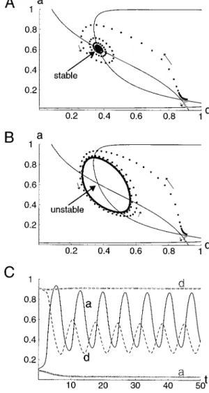
Finally, for some intermediate values of, there can be three steady states, as shown on Figure 6,AandB. In bothAandB, the lower steady state is stable, and the intermediate one (very close to the low state) is unstable. However, the stability of the high-level steady state depends on the particular values of the other parameters. An important parameter, which does not change the location of the steady states, isd. The high-level steady state is stable in Figure 6A, for a value ofd⫽1. Hence, the system is bistable. If the value of d is increased, the negative feedback
caused by depression is more delayed, which can lead to oscilla-tions around the steady state (now unstable), as shown in Figure 6B. The system is bistable again, but now we have a low-activity steady state coexisting with a high-activity oscillatory state. De-pending on the initial conditions (or external inputs), the system can either reach the low steady state or the high activity state, either steady (Fig. 6A) or oscillatory (Fig. 6B,C).
We summarize this collection of possible behaviors in a bifur-cation diagram (Fig. 7A) by plotting the a-values for the steady and oscillatory states when the parameter is varied. The Z-shaped curve (black solid lineand dashes) for steady states is analogous to the S-curve of Figure 3C; the orientation is left– right-reversed because increasingreduces network excitability,
Figure 5. Dynamical behavior of thea⫺dsystem for high(0.28).A, Time course for two different initial conditions. In one case,a(0) is above a threshold, and the network exhibits a transient high-activity phase and then falls to quiescence (black curves). In the other case, the network goes directly to “rest” (gray curves).ais indicated by thesolid curves;dashed curvesrepresentd.B, Phase-plane representation of the dynamics, show-ing trajectories for the two cases illustrated inA. There is only one steady state, defined by the intersection of thed-nullcline and the lower branch of the a-nullcline (for a ⯝ 0)—the quiescent state. If the system is perturbed away from steady state by a sudden increase in activity, the threshold for generation of a transient cycle of high activity is approxi-mately given by the middle branch of thea-nullcline (it is actually slightly above).n⫽1.
Figure 6. Dynamical behavior ofa⫺dsystem for intermediate(0.2). A, Phase-plane representation of the dynamics ford⫽1. The high and
low steady states are stable. Any trajectory eventually reaches one of them, depending on initial conditions. A perturbation away from the low steady state can switch the system to the high state, if it is above the middle branch (black trajectory). Otherwise, the system falls back to the lower state (gray trajectory).B, Phase-plane representation of the dynamics for d⫽2. This higher value destabilizes the high steady state and leads to the
appearance of a stable oscillation (closed orbit) around it. Again, a suffi-cient perturbation can switch the system from the low-activity steady state to oscillations.C, Time courses for the trajectories shown inB. Super-threshold perturbation leads to an oscillation (black curves), whereas after a subthreshold perturbation, activity returns directly to the low steady state (gray curves). Thedashed curvesrepresentd.n⫽1.
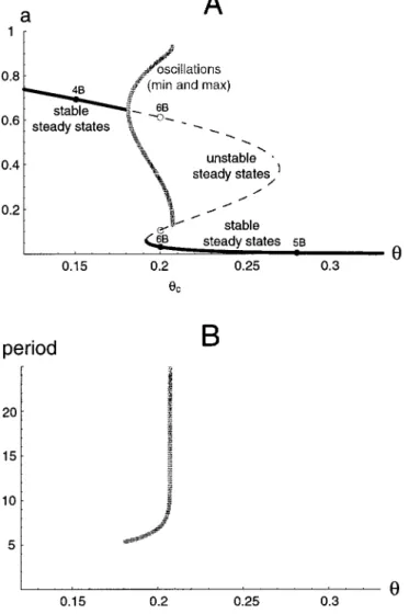
like decreasingn. Starting atlow with the unique high-activity steady state and moving rightward along this curve, we see that this state loses stability at⬎0.181 (solidturns todashed). At this point, a stable oscillation emerges, around the steady state. We plot the maximum and minimum values ofaduring a cycle (thick gray curves). At emergence, the oscillation’s amplitude is very low, but then grows as increases. This type of oscillation birth is called a Hopf bifurcation (Rinzel and Ermentrout, 1998). At a critical value of (c ⫽ 0.207), the oscillation encounters the unstable state on the Z-curve’s middle branch and disappears. That is, the minimum activity during a cycle is just equal to the excitation threshold, and the oscillation cannot be maintained if
is increased any farther. For largeronly the low-activity steady state is stable.
The system is bistable forbetween the Z-curve’s left knee and
c. Over this range, it can be either at a low, steady activity level, or at a high, oscillatory level. These high-activity oscillations
mimic the cycling observed during an episode of activity in the chick spinal cord. In the next sections we will see how slow autonomous dynamics for this modulatory variablecan sweep thea⫺dsubsystem back and forth over this bistable regime to account for the cord’s episodic rhythms. Thus, although Figure 7Adoes not show motion per se, it forms the skeleton over which episodic dynamic patterns can be understood. For example, as shown from Figure 6A,B, the value ofwhere the cycles emerge depends on parameters such asd. Ifdis decreased, the oscilla-tions emerge for higher values of . Consequently, when an episode is started, the system first jumps toward a high stable steady state, then with increasedthis high state becomes unsta-ble and oscillations emerge. Thus, our model when the slow variable is included may exhibit, depending on parameter values, episodes that have phases of near steady high-activity before oscillations start, as sometimes seen experimentally (Fig. 1, bottom panel).
Figure 7Bshows the variations of oscillation period with. For the lowest possible value ofallowing oscillations, the period is finite. The period lengthens asincreases, first slowly and then abruptly just before the oscillations disappear (it becomes infinite at the exact point where the low oscillatory level meets the intermediate, unstable state). Except for the very end of the range, the cycle period ranges between 5 and 10 units of time (approximately 7 for the activity shown on Fig. 6C). Therefore, because the typical cycle period measured experimentally is⬃1 sec for embryonic day (E) 10 embryos,d⫽2 predicts that the time constant of the depression variable d is of the order of 200–400 msec. This is comparable to time scales reported in other systems (Chance et al., 1998).
Slow activity-dependent depression leads to episodic behavior
In the chick embryo, after an episode of activity, evoked mono-synaptic and polymono-synaptic potentials are depressed and recover with a time constant of ⬃1 min (Fedirchuk et al., 1999). In addition, after an episode, the membrane potential of ventrally located spinal neurons hyperpolarizes and subsequently recovers as a depolarizing ramp until the next episode. Collectively, these observations indicate the presence of a slow (time scale minutes) activity-dependent form of depression that regulates network excitability and has been proposed to control the occurrence of episodes (O’Donovan and Chub, 1997). Although the mecha-nisms for these changes are unknown, they could occur through a modulation of cellular properties or a prolonged “slow” form of synaptic depression. In the following, we formulate and analyze models for each of these two possibilities.
The two-variable system presented in the previous section models a bistable, recurrent excitatory network that can exhibit persistent states of low and high activity, the latter being oscilla-tory. In contrast, the chick’s spinal cord shows spontaneous alter-nation between two such states. Here, we add a slow, third variable that enables the model to generate sustained, repetitive episodes of cycling at high activity separated by low-activity phases, thereby mimicking the spontaneous, episodic rhythm of the cord. We show that the mathematical structure that underlies the episodic behavior is the same for both types of slow activity-dependent depression. Therefore, the two models behave in sim-ilar ways, say, when perturbed by a brief stimulation or noisy input, and they are affected similarly by some parameter varia-tions. In a later section, however, we show that the models lead to
Figure 7. A, Bifurcation diagram showing the possible behaviors of the a⫺dfast subsystem for different values of. For low values of, there is only one steady state, at high level, which becomes unstable for increasing . For intermediate values of(around 0.2), the system is bistable: there is a stable high-activity oscillation and a stable, low steady state. With larger values of, the system can only be in a low steady state.Circles represent the cases shown in Figures 4B, 5B, and 6B.Thick black curves: stable steady states;dashed,thin curve: unstable steady states;thick gray curve: maximal and minimal values ofafor the periodic oscillations.B, Period of the oscillations.
different predictions for variations in connectivity and therefore the models can be distinguished experimentally.
Slow modulation of cellular excitability:-model
Intracellular recordings have shown that there is a slow ramp depolarization in motoneurons of chick embryonic spinal cord (N. Chub and M. J. O’Donovan, unpublished observation), sug-gesting that after an episode the functional threshold () of neurons is raised and slowly decreases until the next episode. We can therefore imagine that increases during an episode and decreases during the silent phase. This means that the growth and decay ofis activity-dependent, analogous to a slow adaptation mechanism. During high activity the threshold rises, eventually terminating the activity, and then it recovers during the interepi-sode quiet phase. When the threshold decreases adequately, the network’s small amount of spontaneous activity can trigger an-other episode. We formulate below a kinetic model for that yields this behavior.
From our dynamical systems viewpoint and the previous sec-tions, we can predict the model system’s behavior as follows (we will confirm this below in Figure 8 with a simulation). First, because will move very slowly, we expect that the a ⫺ d subsystem will evolve relatively rapidly to one of its two attractors (Fig. 7A) and then track it asmoves. Suppose the network is in the low-activity state, as after an episode. Under this condition
will slowly decrease, and thea⫺dsubsystem will slowly track the Z-curve’s lower branch until the left knee is reached. The system then rapidly moves to the oscillatory high-activity state, starting an episode. During the episodenow increases, and as indicated by thethick gray curveson Figure 7A, the cycle amplitude also gradually increases. Moreover, the cycle period increases too (Fig. 7B), but only slightly at the beginning of the episode, then significantly near the end of the episode. Note, this significant drop in period just before episode termination is a generic feature of this type of model and is typical of many experiments in chick cord (Fig. 1,top panel). Eventually,reaches the critical levelc where activity can only jump back to the lower steady state, terminating the episode. As then decreases again (recovery), the process will be repeated. Thus, the presence of bistability of thea⫺dsubsystem for a range ofvalues suggests a mechanism for the slow occurrence of episodes, in the same way that the bistability of the simple recurrent network over a range of con-nectivity values suggested a mechanism for the generation of cycles during an episode. Our prediction of the slow rhythm’s a⫺trajectory rests on the assumptions (i.e., on our construc-tion) that (1) the fasta⫺dsubsystem is bistable, (2)evolves very slowly, and (3)evolves in the proper directions during the active and quiescent phases. These features form the essence of the fast/slow dissection technique for analyzing multiple time scale oscillations and excitability of this sort (Rinzel and Ermentrout, 1998).
As for aand d, we model the variations ofwith a simple, first-order kinetics:
˙⫽⬁共a兲⫺, (3)
with⬁an increasing (sigmoidal) function ofaandbeing two to three orders of magnitude greater thana. Thuswill increase from low values if activity is high and decrease from high values if activity is low.
The time courses ofaandfor the full three-variable model resulting from the interaction of thea ⫺d fast subsystem and
the slowsubsystem are shown in Figure 8A. As expected, the behavior is episodic, with rhythmic cycling during episodes. The system’s trajectory actually lives in the three-dimensional phase space,a⫺d⫺. In Figure 8Bwe project the trajectory onto the (a⫺) plane, enabling us to see the dynamic behavior along with the static bifurcation diagram from Figure 7A. We see qualita-tively what we anticipated in the preceding paragraphs, with
covering the bistable range back and forth. Although the trajec-tory does not exactly follow the bifurcation diagram, it would if we had madelarger.
It is important to emphasize that both onset and termination of the episodes are controlled by the value of, as shown from the trajectory in the (a⫺ ) plane. Also shown in Figure 8Bis the
-nullcline, the set of points for which˙⫽0, that is,⫽⬁(a).
Below this nullcline,˙⬍ 0, thereforeis decreasing, and con-versely, for any point above the nullclineis increasing. Thus,
decreases during the silent phase and increases during an epi-sode. Obviously, the position of the -nullcline relative to the a⫺dbifurcation diagram is critical for the existence and timing of episodic rhythmicity (see below).
Figure 8. A, Time courses ofaandfor the-model. During an episode increases, until the episode stops.B, Corresponding trajectory in the (a,) plane, superimposed on the bifurcation diagram. Also plotted is the -nullcline (dot–dashed curve). Below this nullcline, the trajectory flows leftward (˙⬍0, recovery during the silent phase); above it the trajectory flows rightward (˙⬎0, depression during an episode). The points num-bered1,2,3, and4correspond to the same states of the network on both AandB. During an episode, the trajectory passes sequentially1–2–3–4; during a silent phase it goes from4to1.
This graphical representation allows one to easily predict/ understand the effect of parameter variations on the episodic rhythm. Suppose the cellular adaptation is recruited more easily (say,is decreased). This lowers the-nullcline. If it drops too much it will intersect the Z-curve’s lower branch. At this inter-section, all variables, including, are at a stable steady state of low activity; the network will remain silent. On the other hand, if the
-nullcline is too high,can stop increasing before the end of the episode, and the network might enter continuous oscillation. Therefore, the position of the nullcline, or in other words, the value ofafor which the average cellular excitability in the net-work starts to get depressed, has to be within a certain range for episodic oscillations to occur.
The episode durations and silent phase lengths depend on two factors. First, they depend on the rangeof values that covers between the beginning and end of the episodes, that is, the horizontal distance between points4and1on Figure 8B. Increas-ing this range dilates both the episode and silent phase in the same way, because the paths 1–2–3–4 and 4–1 are increased accordingly. As illustrated below, this range can be changed by varying any single parameter of the fast subsystem. Second, the episode durations and silent phase lengths depend on thevelocity with whichvaries. Because this velocity is inversely proportional to, an increase in this time constant increases similarly the time it takes to depress the network and the recovery period, so both duration and silent phase change by the same factor. However, this velocity is also proportional to the horizontal distance be-tween the current point in thea⫺ plane and the-nullcline, because˙⫽⬁(a)⫺. Therefore, if the nullcline is changed
[that is, the function⬁(a) is changed], velocities are modified.
However, this change in the velocity depends on the activity state (high or low) of the system. For example, if the nullcline is moved down, the velocity decreases during the silent phase because
⬁(a)⫺is reduced, but increases during the episode because
⬁(a) ⫺ is increased. Therefore, episode and silent phase
lengths may be affected in opposite ways when a parameter of the slow subsystem is changed. The distinction between the effects of parameters of the fast versus slow subsystems will be important subsequently to distinguish the two models.
Long-term synaptic depression:s-model
As was considered previously, it is also possible to interpret the slow form of activity-dependent depression as arising synaptically rather than from a slow modification of cellular thresholds. In-deed, this mechanism has been proposed to account for the slow recovery of synaptic potentials after an episode (Fedirchuk et al., 1999). Callingsthe new, slow variable, the system becomes:
aa˙⫽a⬁共n䡠s䡠d䡠a兲⫺a dd˙⫽d⬁共a兲⫺d
ss˙⫽s⬁共a兲⫺s.
As ford, a high value ofs(near 1) means “not depressed,” sos⬁
is a decreasing function of a. Note that the fraction of nonde-pressed synapses is nows䡠d, and the effective connectivity isn䡠s䡠d. The activity obtained with this model is qualitatively similar to the one obtained with the-model, as shown in Figure 9. Here again, the onset and termination of episodes are controlled by the slow depression variable (s), therefore silent phase and episode durations are determined in the same way. The reason the
-model and the s-model are so similar is that variations of s
induce the same qualitative changes in the dynamics of the fast subsystem as do variations of. Note that because depression is associated with smaller values of s, in contrast to the-model where largemeans larger depression, the bifurcation diagram of Figure 9Bhas opposite (left/right) orientation to that of Figure 8B. Simulation experiments with the models
To further characterize the models’ behaviors and compare them with experimental data, a few manipulations were conducted. The model network can be perturbed by a brief stimulation. It is also important to understand how the model is affected by varying its parameters, because the parameter variations may be identified with experimental manipulations or with evolving system condi-tions that occur during development. In addition to the
compar-Figure 9. A, Time courses ofaandsfor thes-model. During an episode sdecreases, until the episode stops. As for the-model (Fig. 7B), the cycle period increases near the end of an episode. A little after t⫽ 400, a stimulation was applied, which triggered an episode. This episode was shorter because recovery ofswas not complete.B, Corresponding trajec-tory in the (a,s) plane, superimposed with the bifurcation diagram and the s-nullcline (dot–dashed curve). C, Recordings from an E10 cord. Stimulating quickly after a spontaneous episode triggers a short episode. Black trianglesindicate time of stimulation.
ison with experimental data, the following simulations offer some predictions that are testable experimentally.
Activity resetting.In the chick spinal cord, it is easy to trigger an episode during a silent phase with a brief electrical stimulus. In addition, if the stimulation is applied shortly after a spontaneous episode, the evoked episode is much shorter than the average spontaneous episode, as illustrated on Figure 9C. This effect was observed on all preparations tested (⬎20). It is to be expected if the silent phase is a period of recovery from depression, and it is indeed a characteristic feature of the models presented here. We have illustrated this point for thes-model on Figure 9A,B. Again exploiting the graphical representation of Figure 9B, we see that to evoke an episode the stimulus must be substantial enough to bring the activity above the S-curve’s middle branch. Otherwise, activity returns immediately to the low steady state. Because the vertical distance between the unstable steady state and low-activity state is highest just after an episode and progressively declines, the smaller the amount of time after an episode, the harder it is to successfully evoke a new episode, in agreement with experiments. These results are also observed with the-model because it relies on the same mechanism of episode generation.
Changing a parameter of the fast subsystem. The main effect of changing one parameter of the fasta⫺dsubsystem is to change the values of the slow variable at the beginning and/or end of episodes (or, equivalently, at the end and beginning of silent phases) by deforming the shape of the bifurcation diagram and, in many cases, without moving it much relative to the slow variable’s nullcline. Therefore, as mentioned above (section describing the
-model), silent phase and episode duration are affected in the same way, because the slow variable runs through the same range during the episode and the silent phase.
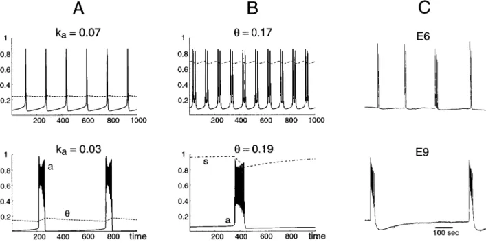
Figure 10 illustrates the effects of changing parameters in the fast subsystem: the steepness ofa⬁(a) for the-model (Fig. 10A)
and the value offor thes-model (B). Increasing the steepness (decreasingka; see Materials and Methods) leads to larger inter-val and episode durations, higher cycling frequency, and larger tonic component. Makinga⬁steeper also results in a lower level
of (background) activity during the silent phase. Increasingin thes-model produces similar effects. These increases in interval and episode duration, cycling frequency, and tonic component are observed experimentally with development, as shown in Figures 1 and 10C [see also O’Donovan and Landmesser (1987)]. For instance, activity at E4–5 consists of single cycle episodes, lasting just a few seconds, but recurring with intervals of⬃2 min (Milner and Landmesser, 1999). By E10–11, episodes typically last⬃60 sec, with intervals of 15–20 min.
To understand more physiologically how such a change in a parameter of the fast subsystem affects both episodes and inter-vals in the same way, let us consider the example of varyingfor thes-model (Fig. 10B). To keep the argument simple, we exag-geratedly assimilate the effect on episode termination to the effects on the high-activity states. Obviously, if the cellular thresh-oldis increased,swill need to reach a higher value to start an episode, because neurons will require a higher level of excitation to start firing. However, the value ofsthat terminates the episode will not be increased as much by the increase of. The reason is that during an episode neurons receive huge synaptic inputs, bringing them far above threshold. A small change intherefore does not affect very much the activity during an episode. In other words, the high-activity states are rather insensitive to changes in
, as can be seen from the saturating shape of a⬁(Fig. 2C) for
large inputs. This is also illustrated in thea–dplane; note how the bottom part of thea-nullcline is much more shifted to the right than the top part whenis increased (Figs. 4B, 5B). The conse-quence of the need to recover more from depression before starting an episode, although the level of depression terminating
Figure 10. Time courses of activity (solid curves) and slow process (dashed curves) for different values of a parameter of the fast subsystem.A, Increasing the slope ofa⬁increases both interval and episode duration (-model). The intermediate caseka⫽0.05 was shown on Figure 8A. Other parameter values
are given in Table 1.B, For thes-model, increasingleads to longer silent phases and longer episodes. Notice how the increases in interval and duration are paralleled by an increase in the range covered by the slow variable. The intermediate case⫽0.18 was shown on Figure 9A. Other parameter values are given in Table 1.C, Spontaneous activity recorded from chick embryonic cord at two stages of development showing the increases in silent phase and episode duration. The scale bar applies to both traces.
the episode is not changed much, is that intervals will be longer, and so will episodes be. The increased level of effective connec-tivity needed to start an episode for increased cellular threshold also means increased synaptic drive at the beginning of an epi-sode and thus explains the larger tonic components for higher. A lower level of “background” activity just after an episode is also attributable to the increased value of , because for a higher cellular threshold, in the absence of network activity the number of cells firing randomly will be even smaller. Again this can be seen from thea⬁curve (Fig. 2C), which shifts to the right when
increases, or in thea–dplane by comparing Figures 4Band 5B. Note how the lower branch of thea-nullcline, and therefore the low state, is almost down to 0 for the higher.
We have also seen that a decrease indleads to similar effects, and so does an increase ind(data not shown). These results suggest that developmental changes that affect the fast subsystem (time scale ⬍1 sec) could be responsible for the increase of episode duration and interepisode interval (time scale minutes), as well as an increase of the tonic component, with age. This prediction is testable by comparing the time constant of fast depression (for example) at different stages of development. The model also suggests that these developmental changes are accom-panied by a reduction in the background activity during the silent phase. Again this could be tested experimentally with intracellu-lar or optical recordings.
Distinguishing the two models
To summarize our previous results, we have constructed two models of episodic oscillatory activity. They share common rhyth-mogenic properties. Their cycle-generating fast subsystems, re-flecting the interplay of a regenerative activity attributable to recurrent excitatory connections and (fast) synaptic depression, are bistable (coexistent states of cyclic high activity and near quiescence). The episodic nature of the activity results from the addition of a slow, activity-dependent process, in one case a slow modulation of cellular properties (-model) and in the other case a slow synaptic depression (s-model). Both models have similar
dynamics, where the slow process switches the network between low and high activity states. As a result, changing a parameter of the fast subsystem affects interepisode interval and episode du-ration in the same way for both models.
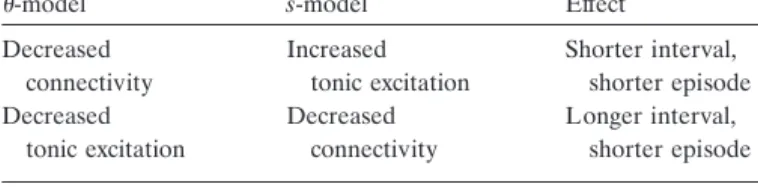
How can we distinguish between the two models? What exper-iment would manipulate a parameter that has different effects on the-model than on thes-model? We have seen that varying a parameter of theslowsubsystem could affect interval and dura-tion in opposite ways. Therefore, varying a parameter that is in the fast subsystem for one model and in the slow subsystem for the other model could have different effects on the models. In this last section, we show that the connectivity parameter,n, affects both models in a different way and also has experimental relevance. Applying the graphical analysis used in the previous sections, we show that only thes-model can explain adequately the experi-mental data, specifically the effects induced by a reduction of synaptic transmission.
Becausencan be identified with the number of connections in the network, it is suitable for experimental manipulation. One way to accomplish this is to antagonize synaptic receptors. For instance, it has been shown previously that on application of the NMDA receptor antagonist APV (alone or in conjunction with CNQX) the activity stops for a period of time but then recovers, with moderately longer interepisode intervals than in control conditions (accompanied by a slight decrease in episode duration) (Barry and O’Donovan, 1987; Chub and O’Donovan, 1998a). We therefore have redone these experiments (using only APV) and compared the results with a decrease ofnfor both models (Fig. 11). All of four experiments on E9–10 preparations showed the transient cessation of activity after drug application, followed by recovered activity with moderately longer intervals than control (after recovery, there was also a slow decrease of the intervals with time, such that in one of the experiments the average interval after recovery was equal to the average control interval).
Both models reproduce the transient cessation of activity after a decrease in connectivity, although it is less marked for the
Figure 11. Effect of a reduction of connectivity.A, Experimental results from an E10 chick spinal cord on application of 100MAPV.Top trace represents electrical activity recorded from a ventral root.Bottom plotrepresents, for each episode, the length of the preceding interval. Over four experiments, control interval, pause, and “recovered” intervals were 742⫾170, 3400⫾970, and 970⫾190 sec, respectively (mean⫾SEM).B,Top, Time course of activity for thes-model on a decrease ofnfrom 1.2 (“control”) to 0.9 (⫺25%).Bottom, As onbottom plotofAfor thes-model (filled symbols) and the-model (open triangles).
-model. More importantly, the following intervals are paradox-icallyshorterthan control for the-model, whereas they arelarger for thes-model, as observed experimentally. Also, episode dura-tion decreases markedly for the-model, in contrast to the slight decrease observed experimentally. These results suggest that the s-model is in better agreement with the data than the-model. The effects of varyingnon both interepisode interval and episode duration are summarized in Figure 12. The models clearly differ in the way intervals are affected. For the-model, episode dura-tion and interepisode interval are both decreased when connec-tivity is reduced, whereas for thes-model, interval increases for a moderate range ofnand duration only slightly decreases.
The fast/slow dissection approach and associated bifurcation diagrams enable us to understand these results. Figure 13 shows explicitly how changing the connectivity,n, affects the solution skeleton of thea⫺dfast subsystem for the-model. With greater connectivity, activity can start for a higher value ofand can also be sustained for higher values of, because of the higher synaptic drive. However, the value ofc(at an episode’s end) increases more than the value ofat the Z-curve’s left knee (at an episode’s beginning). This means that the bistable range, which is covered by the slow variable during episode and silent phase, is in-creased for inin-creasedn, as shown on the Figure (horizontal bars). Therefore, because the same range is covered during the episode and during the silent phase, both silent phase and episode dura-tion are increased. Note however that the range covered byis also slightly shifted to the right for largern. This slightly increases the horizontal distance from thenullcline (and therefore speed) during a silent phase and decreases it during an episode. There-fore this further increases the duration of an episode but limits the extent of an interval, as shown on Figure 12. There is a lower limit on the connectivity that allows episodic rhythmicity. Ifnis too small the Z-curve’s lower branch intersects the-nullcline, forming a steady state of the whole system. Therefore the network remains at this low activity level. If the-nullcline were higher,n could be decreased further, but for n too low the bistability disappears and so does episodic activity.
We can now explain in a more intuitive way the effect of
connectivity changes. Increasing connectivity implies a higher synaptic drive, and therefore episodes are sustained until the cellular threshold reaches a higher critical value than for lowern. However, the value ofthat has to be reached to start an episode does not increase as much because during the silent phase activity is low, and therefore increasing connectivity does not increase synaptic drive as much as during an episode. Because with higher connectivity episodes start at approximately the same value of, but end for a higher valuec, their duration is increased. In turn, silent phases start at a higher value of the threshold, so they increase in duration too. Note how an increase of connectivity for the-model is analogous to an increase infor thes-model (Fig. 10B). The duality of effects of and n on the two models is discussed in the Appendix. It is this duality that allows us to distinguish the two models.
In thes-model,ncan be identified as a parameter of theslow subsystem. Changing this parameter can thus affect episode du-ration and interepisode interval in opposite ways. To demonstrate this, let us define a new variable s˜ ⫽ n䡠s. The system then becomes:
Figure 12. Episode duration and interepisode interval as a function of connectivity for the two models.A,-model. Both duration and interval increase with increasedn, with a relatively smaller effect on interval.B, s-model. Although duration increases slightly, interval decreases with increasingn.
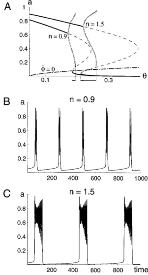
Figure 13. Effects of changing connectivity in-model.A, Bifurcation diagrams corresponding to two different values ofn. Changingnmainly scales the diagram and slightly moves it to theright. The main effect is on the range of bistability, indicated by horizontal bars. Therefore silent phase and duration are changed in the same direction.B, Time course of network activity forn⫽0.9.C, Time course forn⫽1.5.
aa˙⫽a⬁共s˜䡠d䡠a兲⫺a dd˙⫽d⬁共a兲⫺d
ss˜˙⫽n䡠s⬁共a兲⫺s˜,
so that a variation ofnresults only in a multiplicative scaling of thes˜-nullcline, as shown in Figure 14A. From this diagram it is easily seen that the range of s˜does not change withn, but the relative speeds of s˜ are affected. During the silent phase the distance between the trajectory and thes˜-nullcline is smaller for smallern, implying a lower velocity during recovery. Therefore, when connectivity is lowered, interval increases. At the same time, episode duration slightly decreases (Figs. 12, 14B,C). The reason for only a small effect on duration is that during activity, s⬁(a)⯝0, so multiplying it byndoes not change it much, implying
that the part of thes˜nullcline relevant to high activity is moved only slightly leftward (for decreasedn) compared with the part corresponding to the recovery phase.
After application of the glutamate antagonists there is a very large interval, immediately followed by regular occurrence of
episodes. It has been hypothesized previously that the lack of activity for a long period of time (⬃1 hr) could lead to an upregulation of the GABA/glycinergic synapses (Chub and O’Donovan, 1998a). The strengthening of these synapses would compensate for the blockade of the glutamatergic synapses. Our graphical approach helps us to interpret this result with the s-model in a different way. As shown in Figure 15, when n is decreased, the whole diagram is shifted instantaneously to the right, that is, to larger values ofs. However, just after the manip-ulation the variables, because it is slow, will be unchanged. The system’s state drops to the low-activity branch of the shifted S-curve (the only attractor at thiss-value). Before an episode can be initiated,shas to recover to a much larger value (the shifted right knee), hence the long period of inactivity. Oncesis in the right range, episodes occur regularly as in control conditions. Therefore, the model suggests that the hypothesized upregula-tion of GABA/glycinergic synapses may simply be a shift to a lower level of depression.
Finally, there is a corollary to this transient large interval after a decrease in connectivity. Ifnis brought back to its original value, in other words, if the drugs are washed out,shas to decrease back to its original range. Assuming that the washout is immediate,shas to decrease while activity is in the high state. Therefore the model predicts that after washout there should be a very long episode. To test this prediction we have examined the length of the episodes after washing out APV (CNQX was not applied because it washes out too slowly). We did not find such a dramatic increase in the next episode’s duration, probably because the drug does not wash out instantaneously. In two cases, there was a longer episode, but the general effect was a transient reduction of the silent phase. This can be interpreted with the model as a gradual change from the S-curve structure on the right of Figure 15 to that on the left. As the diagram drifts leftward and the trajectory during a silent phase is moving to the right, they intersect, and episodes are started more often than usual, untilsreaches the control range. If we measure the percentage of active phase (the duration divided by the length of the preceding interval), the model predicts a transient decrease in this percentage after drug application and a transient increase after washout. This is what is observed experimentally in all four preparations (data not shown).
DISCUSSION
We have analyzed models that describe the activity of a randomly connected, excitatory network with activity-dependent network depression. The models reproduce many features of the sponta-neous activity generated by developing spinal networks and make a number of experimentally testable predictions. We have used graphical methods to provide insights into the behavior of the models and show that they can account for the newly discovered short-term plasticity (Chub and O’Donovan, 1998a) exhibited by developing spinal networks.
In the first part of Discussion, we will consider the models and the insights that they have provided into the genesis and proper-ties of spontaneously active spinal networks. In addition, we will identify processes of the models with their putative biological equivalents, and we will then discuss some of the specific predic-tions made by using the models. In the second part of Discussion, we will explain some limitations of the models and those aspects of the network behavior that the models cannot account for in their present form. Finally, we will discuss extensions of the model to other spontaneously active networks and compare it to
Figure 14. Effects of changing connectivity ins˜version ofs-model.A, Bifurcation diagram withs˜-nullclines corresponding to two different val-ues ofn. Changingnonly changes the maximal value ofs˜covered by the nullcline. Ifnis further decreased below 0.85, thes˜-nullcline intersects the low steady-state branch so episodic activity ceases.B, Time course of network activity forn⫽0.9.C, Time course forn⫽1.5.