ATOL: Measure Vectorisation for Automatic Topologically-Oriented Learning

(1)

HAL Id: hal-02296513

https://hal.archives-ouvertes.fr/hal-02296513v2

Preprint submitted on 10 Feb 2020

HAL

is a multi-disciplinary open access

archive for the deposit and dissemination of

sci-entific research documents, whether they are

pub-lished or not. The documents may come from

teaching and research institutions in France or

abroad, or from public or private research centers.

L’archive ouverte pluridisciplinaire

HAL

, est

destinée au dépôt et à la diffusion de documents

scientifiques de niveau recherche, publiés ou non,

émanant des établissements d’enseignement et de

recherche français ou étrangers, des laboratoires

publics ou privés.

ATOL: Measure Vectorisation for Automatic

Topologically-Oriented Learning

Martin Royer, Frédéric Chazal, Clément Levrard, Yuichi Ike, Yuhei Umeda

To cite this version:

Martin Royer, Frédéric Chazal, Clément Levrard, Yuichi Ike, Yuhei Umeda. ATOL: Measure

Vectori-sation for Automatic Topologically-Oriented Learning. 2020. �hal-02296513v2�

(2)

ATOL: Measure Vectorisation for

Automatic Topologically-Oriented Learning

Martin Royer Frdric Chazal Clment Levrard

Inria Saclay Inria Saclay Universit Paris Diderot

Yuichi Ike Yuhei Umeda

Fujitsu Laboratories Fujitsu Laboratories

Abstract

Robust topological information commonly comes in the form of a set of persistence di-agrams, finite measures that are in nature uneasy to affix to generic machine learning frameworks. We introduce a learnt, unsuper-vised measure vectorisation method and use it for reflecting underlying changes in topo-logical behaviour in machine learning con-texts. Relying on optimal measure quantisa-tion results the method is tailored to efficiently discriminate important plane regions where meaningful differences arise. We showcase the strength and robustness of our approach on a number of applications, from emulous and modern graph collections where the method reaches state-of-the-art performance to a ge-ometric synthetic dynamical orbits problem. The proposed methodology comes with only high level tuning parameters such as the total measure encoding budget, and we provide a completely open access software.

1 Introduction

Topological Data Analysis (TDA) is a field dedicated to the capture and description of relevant geometric or topological information from data. The use of TDA with standard machine learning tools has proved partic-ularly advantageous in dealing with all sorts of complex data, meaning objects that are not or partly Euclidean, for instance graphs, time series, etc. The applications

Manuscript currently under review.

are abundant, from social network analysis, bio and chemoinformatics, to medical imaging and computer vision, to name a few.

Through persistent homology, a multi-scale analysis of the topological properties of the data, robust and stable information can be extracted. The resulting features are commonly computed in the form of a persistence diagram whose structure (an unordered set of points in the plane representing birth and death times for the features) does not easily fit the general machine learning input format. Therefore TDA is generally combined to machine learning by way of an embedding method for persistence diagrams.

Contributions. Our work is set in that trend. First using recent measure quantisation results we introduce a learnt, unsupervised vectorisation method for mea-sures in Euclidean spaces of any dimension (Section 2.1). Then we specialise this method for handling persistence diagrams (Section 2.2), allowing for easy integration of topological features into challenging ma-chine learning problems with theoretical guarantees (Theorem 1). We illustrate our approach on a set of experiments that leads to state-of-the-art results on difficult problems (Section 3). Lastly we provide an open source implementation and notebook.

Our quantisation of the space of diagrams is statis-tically optimal and the resulting algorithm, a simple variant of the Lloyd’s algorithm, is simple and efficient. It can also be used in a minibatch fashion, making it practical for large scale and high dimensional problems, and competitive with respect to more sophisticated methods involving kernels, deep learning, or compu-tations of Wasserstein distance. To the best of our knowledge, our results provide the first vectorisation method for persistence diagrams that is proven to be able to separate clusters. There is little to no tuning to this method, and no knowledge of TDA is required for this framework.

(3)

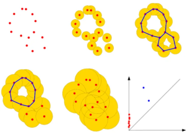
Figure 1: Example of a filtration by union of balls built on top of a 2-dimensional data set (red points) and its corresponding persistence diagram. As the radius of the balls increases, the connected components initially represented by each data point get merged; two cycles appears and disappears along the filtration. The connected components give rise to the red points on the vertical axis of the diagram as their birth time are all 0, and the cycles give rise to the two blue points.

Related work. Finding representations of persistence diagrams that are well-suited to be combined with stan-dard machine learning pipeline is a problem that has attracted a lot of interest these last years. A first fam-ily of approaches consists in finding convenient vector representations of persistence diagrams. For instance it involves interpreting diagrams as images in [AEK+_17],

extracting topological signatures with respect to fixed points whose optimal position are supervisedly learnt in [HKNU17], a square-root transform of their approx-imated pdf in [AVRT16].

A second family of approaches consists in designing spe-cific kernel on the space of persistence diagrams, such as the multi-scale kernel of [RHBK15], the weighted Gaussian kernel of [KHF16] or the sliced Wasserstein kernel of [CCO17]. Those techniques have state-of-the-art behaviour on problems, but for drawback they require another step for an explicit representation, and are known to scale poorly.

A recent other line of work has managed to directly combine the uneasy structure of persistence diagrams to neural networks architectures [ZKR+_{17], [CCI}+_19].

Despite their successful performances, these neural networks are heavy to deploy and hard to under-stand. They are sometimes paired with a representation method as in [HKNU17], [HKN19].

Persistent homology in TDA

Persistent homology provides a rigorous mathematical framework and efficient algorithms to encode relevant

multi-scale topological features of complex data such as point clouds, time-series, 3D images... More precisely, persistent homology encodes the evolution of the topol-ogy of families of nested topological spaces (Fα)α∈A,

called filtrations, built on top of the data and indexed by a set of real numbersA that can be seen as scale parameters. For example, for a point cloud in a Eu-clidean space,Fαcan be the union of the balls of radius

α centered on the data points - see Figure 1. Given a filtration (Fα)α∈A, its topology (homology) changes

asαincreases: new connected components can appear, existing connected components can merge, loops and cavities can appear or be filled, etc. Persistent ho-mology tracks these changes, identifies features and associates, to each of them, an interval or lifetime from αbirth toαdeath. For instance, a connected component

is a feature that is born at the smallestαsuch that the component is present in Fα, and dies when it merges

with an older connected component. The set of inter-vals representing the lifetime of the identified features is called the barcode of the filtration. As an interval can also be represented as a point in the plane with coordinates (αbirth, αdeath), the persistence barcode is

equivalently represented as an union of such points and called the persistence diagram - see [EH10, BCY18] for a more detailed introduction. The classical main advantage of persistence diagrams is that:

(i)they are proven to provide robust qualitative and quantitative topological information about the data [CdSGO16];

(ii)since each point of the diagram represents a specific topological feature with its lifespan, they are easily interpretable as features;

(iii)from a practical perspective, persistence diagrams can be efficiently computed from a wide family of fil-trations [The15].

However, as persistence diagrams come as unordered set of points with non constant cardinality, they cannot be immediately processed as standard vector features in machine learning algorithms. It can be beneficial to interpret persistence diagrams as measures, see for instance [CdSGO16], [CD18], and in this work we will use this paradigm.

Notations

Consider Md the set of finite measures on the d-dimensional ballB(0, R) of the Euclidean space_Rd_with

total mass smaller thanM, for some givenM, R∈R2+.

We assume that the set of input persistence diagrams comes as an i.i.d. sample from a distribution of uni-formly bounded diagrams, that is givenM, R∈_R2

+, let

Dbe the space of persistence diagrams with at mostM points contained in the Euclidean discB2(0, R). The

spaceDis considered as a subspace of the setM2 of

(4)

than M: for any D ∈ D, D :=P

p∈Dδp where δp is

the Dirac measure centered at point p.

2 Methodology

In this section we introduceAtol, a simple unsuper-vised data-driven method for measure vectorisation. Atolallows to automatically convert a distribution of persistence diagrams into a distribution of feature vec-tors that are well-suited for use as topological features in standard machine learning pipelines.

To summarise, given a positive integer b, _Atol pro-ceeds in two steps: it first computes a discrete measure in _Rd _{supported on}_b _{points that approximates the}

av-erage measure of the distribution from which the input observations have been sampled. Second, it computes a set of well-chosen contrast functions centered on each point of the support of this measure, that are then used to convert each observation into a vector of sizeb. 2.1 Measure vectorisation through

quantisation

We now introduce Algorithm 1Atol-featurisation in its generality, that is a featurisation method for ele-ments of Md. The first step in our procedure is to use quantisation in spaceMd. Starting from an i.i.d. sample of measures X1, . . . , Xn drawn from

probabil-ity distribution LX onMd and given an integer

bud-get b∈_N∗_{, we leverage recent algorithms and results}

from [LRC20] and produce a compact representation for the mean measure E(X). That is, we produce a

distribution Pˆcn,b supported on a fixed-length code-book ˆcn,b={c(1), . . . , c(b)} in the ambient space that

aims to minimize over such distribution the distorsion R(Pc) := W22(Pc,E(X)), the squared 2-Wasserstein

distance to the mean measure. In practice, one consid-ers the empirical mean measure ¯Xn and thek-means

problem for this ¯Xn measure. Then the respective

adaptations of Lloyd’s [Llo82] and MacQueen’s [Mac67] algorithms to the format of measures are introduced in [LRC20] and can readily be employed.

From this quantisation our aim is to derive spatial information on measures in order to discriminate be-tween them. Much like one would compactly describe a point cloud with respect to its barycenter in a PCA, we describe measures based on a number of reduced difference to our mean measure approximate. To this end, our second step is to tailorb individual contrast functions each based on the estimated codebook that individually describe local regions. In other words we set to find regions of the space where measures seem to aggregate on average, and build a dedicated descriptor for those regions. We define and use the two following

contrast families R2→R+, fori∈[b]:

These specific contrast functions are chosen to decrease away from the approximate mean centroid in a Lapla-cian (Ψ) or Gaussian (Φ) fashion. We choose the scale to roughly correspond to the minimum distance to the closest Voronoi cell in the corresponding codebook ˆcn,b.

The Ψ-exponential decrease will allow to properly sepa-rate a measure mixture in Theorem 1 so by default we make our arguments with that family in mind and will denote_AtolΦandAtolΨ the Gaussian and Laplacian

versions of the algorithm. To our knowledge there is nothing that prevents other, well designed contrast fam-ilies to be substituted in their place, but this is beyond the scope of this paper. Given a family of contrast function and a mean measure codebook approximate, each element ofMd can now be compactly described through the integrated contribution to each contrast functions: for X∈ Md and contrast function χ, let

X·χ(·,ˆcn,b) :=

Z

x∈Rd

χ(x,ˆcn,b)X(dx). (4)

Our algorithm simply concatenates into a vector each of those contributions.

Algorithm 1:Atol-featurisation

Data: Collection of measuresX1, . . . , Xn∈(Md)n.

parameters :budgetb∈N∗,

contrast familyχ∈ {Ψ,Φ}. Result: vectorisation map v_Atol:Md→Rb.

1 Calibration step 1: apply{batch or minibatch} quantization algorithm of the mean measure with fixed-length support from [LRC20], output: ˆcn,b;

2 Calibration step 2: adjust bmeasurable ”contrast” functions (χi(·,ˆcn,b))i∈[b] to the mean measure

centroids;

3 Vectorisation step: compute featurisation map: v_Atol:Md→Rb, X7→ h X·χi(·,cˆn,b) i i∈[b] .

Calibration step 1 is optimal for deriving space quanti-sation in the following sense: let the excess distorsion be the difference between R(Pˆcn,b) the distorsion of the resulting distribution based on codebook ˆcn,b and

the optimal distorsion of a distribution supported on b points. Then for either version of the quantisation algorithm (batch or minibatch), the excess distorsion

(5)

can be controlled (respectively with high probability or on average) at a logn/nminimax speed under margin conditions, see Theorems 4 and 5 from [LRC20]. 2.2 Topological learning

We now specialise our featurisation method to the context of topological learning when we are set in di-mension d= 2 with D ⊂ M2. Applying Algorithm 1

to a collection from Dis straightforward and allows to embed the complex, unstructured space Din Eu-clidean terms. Set in the context of a standard learning problem, we introduce Algorithm 2 _Atol: Automatic Topologically-Oriented Learning. Let Ω := (X, y) with given observationsX in some spaceX corresponding to a known, partially available or hidden labely∈ Y. As-sume that one has a way to extract toplogical features fromX, i.e. to derive a collection of diagrams associ-ated to those elements, and letκ:X → D, X7→D(X) be the corresponding map. Then applying Algorithm 1 to the resulting collection of diagrams provides some simplified topological understanding on elementsX of this problem.

Algorithm 2: _Atol: Automatic Topologically-Oriented Learning

Data: Learning problem Ω := (X, y)

withX ∈ X observations andy∈ Y labels. parameters :κ:X → Dyielding topological

descriptors, and budgetb∈_N∗_.

Result: Enhanced learning problem

e

Ω := ((X, v_Atol◦κ(X)), y) with euclidean, topological featuresv_Atol◦κ(X)∈_Rb_.

1 Compute intermediate learning problem

ΩPH:= ((X, κ(X)), y)∈(X × D)× Ywith persistent

homology features, unfit for general machine learning routines;

2 Use Algorithm 1 to transform it into a generic machine learning problem

e

Ω := ((X, v_Atol◦κ(X)), y)∈(X ×Rb)× Y.

Suppose now that persistence diagrams originate from distinct sources: assume that observed dia-gramsD1, . . . , Dn are sampled with noise from a

mix-ture model D = PL

l=1πlD(l) of distinct measures

D(1), . . . , D(L)— by that we mean that any two mea-sures in this set differ by at least one point. Call Z the latent variable associated to the mixture so that D|Z = l ∼ D(l)_{. The following results ensures that}

v_Atolhas separative power, i.e. that the vectorisation clearly separates the different sources:

Theorem 1(Separation withAtol).

For a given noise level assumingE(D)satisfies some

(explicit) margin condition and fornandblarge enough

there exists a non-empty segment forσ1, . . . , σbin

Equa-tion (1)such that for all i, j∈[n]2, with high probabil-ity:

Zi=Zj =⇒ kvAtol(Di)−vAtol(Dj)k∞61/4, (5)

Zi6=Zj =⇒ kvAtol(Di)−vAtol(Dj)k∞>1/2. (6)

This result follows from Corollary 19 in [LRC20] and the explicit statement of the assumptions and margin conditions are classical but rather technical and are fully described in [LRC20] (see Definition 3 for the margin conditions).

Notice that establishing that a persistence diagram vec-torisation method allows for separation, i.e. that dia-grams from different clusters will be well-discriminated, has never been achieved to our knowledge. It is not sufficient to find a space quantisation that allows to discriminate a collection of diagrams fromD, the vec-torisation based upon this quantisation could still miss a difference of interest depending on the chosen con-trast family Ψ. The above theorem shows that_Atol overcomes this issue.

Note that in order to adjust the values forσ1, . . . , σb

in Equation (1), we use a common heuristic instead of constant values and it is our intuition that the chosen, adaptive values of Equation (3) help the vectorisation perform better than what the theory can predict. We point that as embedding mapv_Atolis automatically computed without knowledge of a learning task, its derivation is fully unsupervised. The representation is learned since it is data-dependent, but it is also agnostic to the task and only depends on getting a glimpse at an average persistence diagram. Using the minibatch quantisation step of [LRC20] is single-pass so the vectorisation algorithm has linear computation time in O(n×M ×b), therefore it is able to handle high-dimensional problems as long as corresponding diagrams are provided.

This featurisation is conceptually close to two other recent works. [HKNU17] computes a persistence dia-gram vectorisation through a deep learning layer that adjusts Gaussian contrast functions used to produce topological signatures much like our Calibration step 2. So in essence our approach substitutes quantisation to deep learning, with no need of supervision and allowing to provide mathematical guarantees. Next, the bag of word method of [ZLJ+_{19] uses an ad-hoc form of}

quan-tisation for the space of diagrams, then count functions as contrast functions to produce histograms as topolog-ical signatures. There are in fact sensible differences, that will ultimately translate in terms of effectiveness: Section 3.1 shows theAtol-featurisation to produce state-of-the-art mean accuracy on two difficult multi-class multi-classification problems (66.9 % on REDDIT5Kand

(6)

51.6 % on REDDIT12K) that are also tackled by those papers where [HKNU17] report a mean accuracy of respectively 54.5% and 44.5%, and [ZLJ+_{19] report an}

accuracy of respectively 49.9% and 38.6%.

3 Competitive TDA-Learning

In this section we demonstrate experimentally the ad-vantages of our approach. We show theAtol frame-work to be competitive and state-of-the-art, but also versatile and easy to use with high automaticity. 3.1 Graph Classification

Learning problems involving graph data are receiving a strong interest at the moment, consider graph classifi-cation: Ω := (X, y)∈ X × Y is a finite family of graphs and available labels and one learns to mapX → Y. Recently [CCI+_{19] have introduced a powerful way of}

extracting topological information from graph struc-tures. They make use of heat kernel signatures (HKS) for graphs [HRG14], a spectral family of signatures (with diffusion parameter t > 0) whose topological structure can be encoded in the extended persistence framework, yielding four types of topological features with exclusively finite persistence. On both those points we refer to Sections 4.2 and 2 from [CCI+19]. Therefore for each graph and HKS diffusion time tthe resulting topological descriptor are four persistence diagrams with all finite coordinates. For the entire set of prob-lems to come we choose to use the same two HKS diffusion times to be .1 and 10, fueling the extended graph persistence framework and resulting in 8 per-sistence diagrams per considered graph. For budget in Algorithm 2 we choose b= 80 for all experiments, which means Algorithm 1 will rely on approximating the mean measure on ten points per diagram type and filtration. We make no use of (and automatically dis-card) graph attributes on edges or vertices that some dataset do possess, and no other sort of features are col-lected, so that our results are solely based on the graph structure of the problems. To sum up, Algorithm 2 here simply consists in reducing the original problem from Ω toΩ := (ve _Atol◦Φ(X), y) withv_Atol◦Φ(X)∈_R80.

We stress that the embedding map v_Atol from Algo-rithm 1 is computed each time using all diagrams from the training set, without supervision. To measure the worth of this embedding in this learning context, we evaluate the featurisation for classification purposes using the standard scikit-learn[PVG+_11]

random-forest classification tool with 200 trees and all other parameters set as default. On each problem we perform a 10-fold cross-validation procedure and average the resulting accuracies; we report accuracies and standard deviations over ten such experiments.

We use two sets of graph classification problems for benchmarking, one of Social Network origin and one of Chemoinformatics and Bioinformatics origin. They include small and large sets of graphs (MUTAGhas 188 graphs,REDDIT12Khas 12000), small and large graphs (IMDB-M has 13 nodes on average,REDDIT5Khas more than 500), dense and sparse graphs (FRANKENSTEIN has around 12 edges per nodes, COLLABhas more than 2000), binary and multi-class problems (REDDIT12Khas 11 classes), all available in the public page [KKM+_16].

Computations are run on a single laptop (i5-7440HQ 2.80 GHz CPU), in batch version for datasets smaller than a thousand observations and mini-batch version otherwise. Average computing time of Algorithm 1 (the average time to calibrate the vectorisation map on the training set then compute the vectorisation on the entire dataset), are: less than .1 seconds for datasets with less than a thousand observations, less than 10 seconds for datasets that have less than 5 thousand observations, 25 seconds for REDDIT-5K, 50 seconds forREDDIT-12K and 110 seconds for the dens-est problem COLLAB. The results presented here are openly accessible (requiring open source library Gudhi [The15] and reproducible with the public repository github.com/martinroyer/atol.

We compare performances to the top scoring methods for these problems, to the best of our knowledge. Those methods are mostly graph kernels methods tailored to graph problems: two graph kernel methods based on random walks (RetGK1, RetGK11 from [ZWX+18]), one graph embedding method based on spectral dis-tances (FGSD from [VZ17]), two topological graph ker-nel method (WKPI-kM and WKPI-kC from [ZW19]), one graph kernel combined with a graph neural network (GNTK from [DHS+_{19]) and one topological}

vectorisa-tion method learnt by a neural network (PersLay from [CCI+_{19]). Competitor accuracy are quoted from their}

respective publication and we detail how they should be interpreted: for RetGK and WKPI and PersLay the evaluating procedure is done over ten 10-fold, just as ours is so the results directly compare; for FGSD the average accuracy over a single 10-fold is reported, and for GNTK the average accuracy and deviations is reported over a single 10-fold as well. When there are two or more methods under one label, we always report the best outcome.

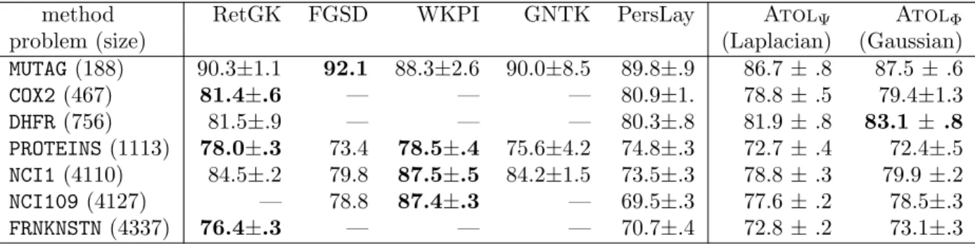
Our results Table 1 are state-of-the-art or substan-tially improving the state-of-the-art on the Large Social Network datasets that are rather difficult multi-class problems. The results on the Chemoinformatics and Bioinformatics datasets Table 2 are state-of-the-art. These results are especially postive seeing how Algo-rithm 1 is generic and has been designed neither for graph experiments nor for persistence diagrams

(7)

specif-method RetGK FGSD WKPI GNTK PersLay AtolΨ AtolΦ

problem (Laplacian) (Gaussian)

REDDIT(5K, 5 classes) 56.1±.5 47.8 59.5±.6 — 55.6±.3 66.9±.3 67±.3 REDDIT(12K, 11 classes) 48.7±.2 — 48.5±.5 — 47.7±.2 51.6±.1 51.6±.2 COLLAB(5K, 3 classes) 81.0±.3 80.0 — 83.6±.1 76.4±.4 87.8±.2 88.1±.1 IMDB-B(1K, 2 classes) 71.9±1. 73.6 75.1±1.1 76.9±3.6 71.2±.7 74.3±.8 74.5±.5 IMDB-M(1.5K, 3 classes) 47.7±.3 52.4 48.4±.5 52.8±4.6 48.8±.6 47.8±.8 48.3±.7

Table 1: Mean accuracy and standard deviations for Large Social Network datasets.

method RetGK FGSD WKPI GNTK PersLay _AtolΨ AtolΦ

problem (size) (Laplacian) (Gaussian)

MUTAG(188) 90.3±1.1 92.1 88.3±2.6 90.0±8.5 89.8±.9 86.7±.8 87.5±.6 COX2(467) 81.4±.6 — — — 80.9±1. 78.8±.5 79.4±1.3 DHFR(756) 81.5±.9 — — — 80.3±.8 81.9±.8 83.1 ± .8 PROTEINS(1113) 78.0±.3 73.4 78.5±.4 75.6±4.2 74.8±.3 72.7±.4 72.4±.5 NCI1(4110) 84.5±.2 79.8 87.5±.5 84.2±1.5 73.5±.3 78.8±.3 79.9±.2 NCI109(4127) — 78.8 87.4±.3 — 69.5±.3 77.6±.2 78.5±.3 FRNKNSTN(4337) 76.4±.3 — — — 70.7±.4 72.8±.2 73.1±.3 Table 2: Mean accuracy and standard deviations for Chemoinformatics and Bioinformatics datasets - all binary classification problems.

ically, and seing how the classification task has been entrusted to an external and generic learning tool. Con-trary to competitors, the method does not require to construct a kernel or a neural network. Overall, the simplicity and absence of tuning hint at robustness and good generalisation power.

3.2 Discrete dynamical systems seen as measures

[AEK+_{17] use a synthetic, discrete dynamical system}

(used to model flows in DNA microarrays) with the following property: the resulting chaotic trajectories exhibit distinct topological characteristics depending on a parameterr >0. The dynamical system is:

xn+1:=xn+ryn(1−yn) mod 1,

yn+1:=yn+rxn+1(1−xn+1) mod 1.

With random initialisation and five different param-eters r ∈ {2.5,3.5,4,4.1,4.3}, a thousand iterations per trajectory and a thousand orbits per parameter, a datasets of five thousand orbits is constituted and commonly used for evaluating topological methods. Figure 2 shows a few orbits generated with parameters r ∈ {4.0,4.1}. For orbits generated with parameter r= 4.1, it happens that the initialisation spawns close to an attractor point that gives it the special shape as in the leftmost orbit. The problem of classifying this datasets in accordance to their underlying

param-Figure 2: Example of synthetised orbits (xandy co-ordinates in the flat torus [0,1]2_{) with parameter 4.0}

(top row) and 4.1 (bottom).

eter is rather uneasy and challenging. Some compet-itive topological methods have tackled this problem in the following way: after a learning phase with a 70/30 split, accuracy with the standard deviation over a hundred such experiments. The following results have been reported: 72.38±2.4 [RHBK15], 76.63±0.7 [KHF16], 83.6±0.9 [CCO17], 85.9±0.8 [LY18], and the state-of-the-art 87.7±1.0 with persistence diagrams in [CCI+_19].

Since those discrete orbits can be seen as measures in [0,1]2_{, we apply our learning framework directly}

on the observed point cloud i.e. we use Algorithm 1 on the synthetic orbits and for learning we use the scikit-learn [PVG+11] random-forest classification tool (with 100 trees and all other parameters set as

(8)

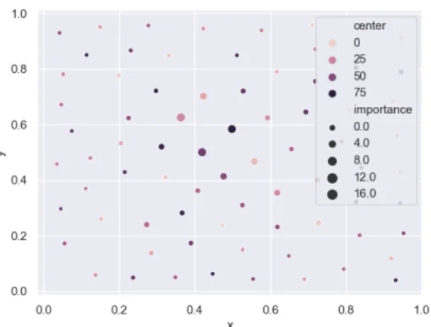
de-Figure 3: Example location ofb= 80 quantisation cen-ters and their respective importance in the clustering task.

fault) on the resulting vector. Note that in this context, our framework resembles that of image classification where instead of a fixed grid for measurement we have learnt centers from which to look at the data. After learning the center importance can be represented (see an example with 80 centers Figure 3) and naturally cen-ters that can gather important geometrical information gain importance in this process.

Using the same 70/30 split procedure and repeating a hundred times with the Ψ-Laplacian contrast family andb= 80 centers (so in the exact same configuration as the graph experiment), we obtain 88.3±.8 mean accuracy and deviation. Therefore our results are also competitive for this high dimensional problem. But what is more, increasing the budget on this experiment yields sensible gains: using the Φ-Gaussian contrast family and a b = 1000 centers for cloud description allows to reach 95% accuracy or more, so it seems that this problem can be precisely described by a purely spatial approach — and our framework can be labeled as such in this context.

We also use this synthetical dataset to present ad-ditional experiments displayed Table 3, designed to understand parameter influence of Algorithm 1. The considered parameters are: (i) a high or low budget b∈_N∗ _{for describing the measure space, (ii) possible}

effect of the contrast functions Ψ or Φ to use for vec-torisation of the quantised space, (iii) the proportion of training observations to use for deriving the quanti-sation, with 10% indicating that all a random selection of a tenth of the measures from the training set were used to calibrate Algorithm 1.

Naturally it is expected that augmenting the budget for vectorising the measure space will yield a better

descrip-tion of said space, and this intuidescrip-tion is confirmed by Table 1. But we stress that a weakness of Algorithm 1 is that once centers are fixed in the quantisation, space regions that are too far from these centers will neces-sarily be left out and the information they can carry with them. Therefore this intuition can sometimes be wrong if a lower number of centers happens to lead to a more pertinent quantisation. Next, the influence of the chosen contrast functions clearly show the Gaussian contrast functions to perform better than the other. Understanding the ability of such contrast functions to describe some particular observation space is challeng-ing and left for future work. Lastly,ORBIT5Kseems to be a dataset where the percentage of observations used in the calibration part of the algorithm does not weigh much on the final result for a budget b= 80 (it does have a significant influence when the budget is lower). This tells us that the calibration can be stable for a given level of information.

3.3 Topological score for time series, an industrial application

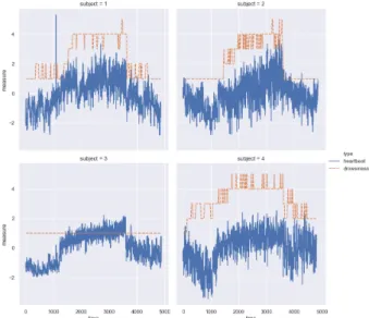
Finally we present an industrial application for time series, in a case where the learning problem is hard and no obvious solutions are to be found. This dataset consists in the following experiments: using commer-cially available simulator of a Japanese city road circuit course, about a hundred subjects are monitored and the intervals between successive heartbeats are recorded (RRI data sampled at 4Hz) for a 80 minutes drive that includes two periods of high-speed driving at the beginning and at the end of the experiment, and a low-speed driving period in the middle designed to induce sleepiness. For each experiment, an expert annotation (labeled NEDO score) produced from visual observation of the driver is made available, indicating sleepiness on a 1 to 5 class scale. We show four such experiments in Figure 4 (the RR-intervals have then been normalised). This problem of retrieving the sleepiness level based on RRI levels is hard and ill-posed: there are strong individual differences in perceived reaction to a given situation, a single experiment per subject to learn be-haviour from, and apparent noise or absence of signal in annotations, see e.g. subject 3 in Figure 4. Nev-ertheless we propose to use the _Atol framework to produce features meant reflect the sleepiness level in subjects based on RRI variations. The intent is that even though this will poorly reflect the latent sleepiness level, this could be enough to allow to catch jumps in the perceived attention level. The framework can read-ily be applied to time series in any given dimension and used to produce topological features. For this applica-tion we will follow a classical path: (i) use a sliding window decomposition on the RRI time-series,(ii) use

(9)

Budget effect Contrast functions Calibration effect b= 2 b= 8 b= 20 b=80 b= 200 Φ-Gaussian Ψ-Laplacian 10% 50% 100% 42.7±.7 68.5±2.5 82.1±2.3 88.3±.8 90.9±.7 93.0±.7 88.3±.8 88.3±.8 88.6±.8 88.6±.8

16.5 s 19.8 s 20.1 s 25.8 s 65.8 s 26 s 25.8 s 25.8 s 25 s 26 s

Table 3: Mean accuracy and deviation and vectorisation time over 10 experiments forORBIT5K. Boldface blue indicate parameters by default, and only one parameter is varied at a time.

Figure 4: Normalized RRI time-series (blue) and anno-tated NEDO score (orange) for four subjects with the simulation time (x-axis, in seconds).

a time-delay embedding to transform said window into a point cloud, (iii)apply persistent homology analysis (we use DTM-filtration [ACG+_{18]) to produce}

persis-tence diagrams and(iv) vectorise persistence diagrams using Algorithm 1.

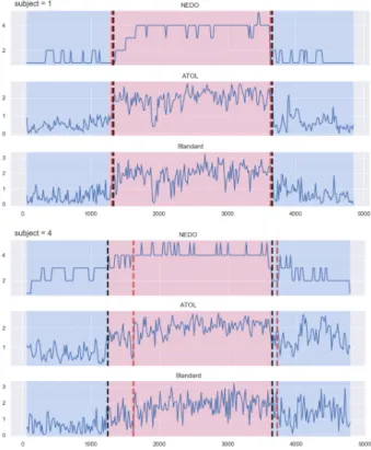
We concatenate those features with the mean and stan-dard deviation statistics on the sliding-window. As for learning, we compute a learner based on other indi-viduals’ features regressed to their NEDO scores, and use it to generate a score based on Atolfeatures (see middle and bottom row in Figure 5). Although this score imperfectly reflects the underlying NEDO score for a given patient, is can still have some uses. We set to detect two jumps on this topologically-augmented score using a Gaussian Kernel. We also compute a regressor based on the standard features without ad-ditional topological features, for comparison purposes, and also detect two jumps on this standard score. Figure 5 shows two example results of our analysis. Each panel (top and bottom) consists in three time-series: the (hidden) NEDO score (top row), the _Atol -score computed from a regressor based on topological features (middle row), and a standard score computed from a regressor based solely on standard features

(bot-tom row). The changes of colour from blue to red and to blue indicates the changes in the experimental design for the driving simulation, i.e. the red portion indicates low-speed driving whereas the blue portions indicate high-speed driving periods. The black dotted lines in-dicate jumps detected from the _Atolrepresentation, whereas the red dotted lines indicate jumps detected from the standard representation. In the top panel, the two series of jumps are concomitant, and almost an exact match to the underlying changes in the exper-imental design. In the bottom panel, an improvement over the standard score is caught with theAtolscore that better reflects the changes in latent NEDO score for this subject, two the point that the detected jumps are an exact match for the changes in experimental conditions. Overall, the _Atol score has less spikes and more regularity than the standard score, which is expected as the topological features are extracted posterior to a time-delay embedding procedure.

4 Conclusion

This paper introduces a vectorisation for measures in Euclidean spaces based on optimal quantisation proce-dures, then shows how this method can be employed in machine learning context and help process topological features. _Atol has a rather simple design, is mul-tifaceted and ties theoretical guarantees to practical efficiency.

Moreover _Atolonly depends on few simple parame-ters, namely the sizeb of the codebook and the choice of contrast functions. The study of the effect and the design of a method for automatic choice of these pa-rameters deserves further analysis and is left to future work.

(10)

Figure 5: For two subjects (1 and 4), results of NEDO score (top row) regression and of a 2-jumps detection procedure, from _Atolprocedure (_Atol-regression in middle row, yields jumps in black dashes) and stan-dard features alone (stanstan-dard-regression in bottom row, yields jumps in red dashes). Red zones indicates low-speed and blue zones indicates high-low-speed section in the experiment.

(11)

References

[ACG+18] Hirokazu Anai, Frédéric Chazal, Marc Glisse, Yuichi Ike, Hiroya Inakoshi, Raphaël Tinarrage, and Yuhei Umeda. Dtm-based filtrations. InSymposium on Computational Geometry, 2018.

[AEK+_17] _{Henry Adams, Tegan Emerson, Michael}

Kirby, Rachel Neville, Chris Peterson, Patrick Shipman, Sofya Chepushtanova, Eric Hanson, Francis Motta, and Lori Ziegelmeier. Persistence images: a sta-ble vector representation of persistent ho-mology. Journal of Machine Learning Re-search, 18(8), 2017.

[AVRT16] R. Anirudh, V. Venkataraman, K. N. Ra-mamurthy, and P. Turaga. A riemannian framework for statistical analysis of topo-logical persistence diagrams. In2016 IEEE Conference on Computer Vision and Pat-tern Recognition Workshops (CVPRW), pages 1023–1031, June 2016.

[BCY18] Jean-Daniel Boissonnat, Fr´ed´eric Chazal, and Mariette Yvinec.Geometric and Topo-logical Inference, volume 57. Cambridge University Press, 2018.

[CCI+19] Mathieu Carrière, Frédéric Chazal, Yuichi Ike, Théo Lacombe, Martin Royer, and Yuhei Umeda. PersLay: A Simple and Versatile Neural Network Layer for Persis-tence Diagrams. To appear in AISTATS 2020, page arXiv:1904.09378, Apr 2019. [CCO17] Mathieu Carrière, Marco Cuturi, and

Steve Oudot. Sliced Wasserstein kernel for persistence diagrams. In Interna-tional Conference on Machine Learning, volume 70, pages 664–673, jul 2017. [CD18] Fr´ed´eric Chazal and Vincent Divol. The

density of expected persistence diagrams and its kernel based estimation. InSoCG 2018 - Symposium of Computational Ge-ometry, Budapest, Hungary, June 2018. Extended version of the SoCG proceed-ings, submitted to a journal.

[CdSGO16] Fr´ed´eric Chazal, Vin de Silva, Marc Glisse, and Steve Oudot.The structure and stabil-ity of persistence modules. SpringerBriefs in Mathematics. Springer, 2016.

[DHS+19] Simon S Du, Kangcheng Hou, Russ R Salakhutdinov, Barnabas Poczos, Ruosong Wang, and Keyulu Xu. Graph neural

tangent kernel: Fusing graph neural net-works with graph kernels. In H. Wallach, H. Larochelle, A. Beygelzimer, F. d’Alch´e Buc, E. Fox, and R. Garnett, editors, Ad-vances in Neural Information Processing Systems 32, pages 5724–5734. Curran As-sociates, Inc., 2019.

[EH10] Herbert Edelsbrunner and John Harer.

Computational Topology: An Introduction. AMS, 2010.

[HKN19] Christoph Hofer, Roland Kwitt, and Marc Niethammer. Graph filtration learning, 2019.

[HKNU17] Christoph Hofer, Roland Kwitt, Marc Ni-ethammer, and Andreas Uhl. Deep learn-ing with topological signatures. In Ad-vances in Neural Information Processing Systems, pages 1634–1644, 2017.

[HRG14] Nan Hu, Raif Rustamov, and Leonidas Guibas. Stable and informative spec-tral signatures for graph matching. In

Proceedings of the IEEE Conference on Computer Vision and Pattern Recognition,

pages 2305–2312, 2014.

[KHF16] Genki Kusano, Yasuaki Hiraoka, and Kenji Fukumizu. Persistence weighted Gaussian kernel for topological data analysis. In In-ternational Conference on Machine Learn-ing, volume 48, pages 2004–2013, jun 2016. [KKM+16] Kristian Kersting, Nils M. Kriege, Christo-pher Morris, Petra Mutzel, and Marion Neumann. Benchmark data sets for graph kernels, 2016. http://graphkernels.cs. tu-dortmund.de.

[Llo82] Stuart P. Lloyd. Least squares quantiza-tion in PCM.IEEE Trans. Inform. Theory, 28(2):129–137, 1982.

[LRC20] Clément Levrard, Martin Royer, and Frédéric Chazal. Optimal quantization of the mean measure and application to clustering of measures, 2020.

[LY18] Tam Le and Makoto Yamada. Persistence Fisher kernel: a Riemannian manifold ker-nel for persistence diagrams. InAdvances in Neural Information Processing Systems, pages 10027–10038, 2018.

[Mac67] J. MacQueen. Some methods for classifi-cation and analysis of multivariate obser-vations. InProc. Fifth Berkeley Sympos.

(12)

Math. Statist. and Probability (Berkeley, Calif., 1965/66), pages Vol. I: Statistics, pp. 281–297. Univ. California Press, Berke-ley, Calif., 1967.

[PVG+_11] _{F. Pedregosa, G. Varoquaux, A. Gramfort,}

V. Michel, B. Thirion, O. Grisel, M. Blon-del, P. Prettenhofer, R. Weiss, V. Dubourg, J. Vanderplas, A. Passos, D. Cournapeau, M. Brucher, M. Perrot, and E. Duches-nay. Scikit-learn: Machine learning in Python. Journal of Machine Learning Re-search, 12:2825–2830, 2011.

[RHBK15] Jan Reininghaus, Stefan Huber, Ulrich Bauer, and Roland Kwitt. A stable multi-scale kernel for topological machine learn-ing. In IEEE Conference on Computer Vision and Pattern Recognition, 2015. [The15] The GUDHI Project. GUDHI User and

Reference Manual. GUDHI Editorial Board, 2015.

[VZ17] Saurabh Verma and Zhi-Li Zhang. Hunt for the unique, stable, sparse and fast fea-ture learning on graphs. InAdvances in Neural Information Processing Systems, pages 88–98, 2017.

[ZKR+17] Manzil Zaheer, Satwik Kottur, Siamak Ravanbakhsh, Barnabas Poczos, Rus-lan Salakhutdinov, and Alexander Smola. Deep sets. InAdvances in Neural Informa-tion Processing Systems, pages 3391–3401, 2017.

[ZLJ+19] Bartosz Zieliski, Micha Lipiski, Mateusz Juda, Matthias Zeppelzauer, and Pawe Dotko. Persistence bag-of-words for topo-logical data analysis. InProceedings of the Twenty-Eighth International Joint Confer-ence on Artificial IntelligConfer-ence, IJCAI-19, pages 4489–4495. International Joint Con-ferences on Artificial Intelligence Organi-zation, 7 2019.

[ZW19] Qi Zhao and Yusu Wang. Learning met-rics for persistence-based summaries and applications for graph classification. In H. Wallach, H. Larochelle, A. Beygelzimer, F. d’Alch´e Buc, E. Fox, and R. Garnett, editors,Advances in Neural Information Processing Systems 32, pages 9855–9866. Curran Associates, Inc., 2019.

[ZWX+18] Zhen Zhang, Mianzhi Wang, Yijian Xiang, Yan Huang, and Arye Nehorai. RetGK:

Graph Kernels based on Return Proba-bilities of Random Walks. In Advances in Neural Information Processing Systems, pages 3968–3978, 2018.