Behavioral/Systems/Cognitive
Higher-Dimensional Neurons Explain the Tuning and
Dynamics of Working Memory Cells
Ray Singh
1and Chris Eliasmith
1,2Departments of1Systems Design Engineering and2Philosophy, University of Waterloo, Waterloo, Ontario, Canada N2L 3G1
Measurements of neural activity in working memory during a somatosensory discrimination task show that the content of working memory is not only stimulus dependent but also strongly time varying. We present a biologically plausible neural model that reproduces the wide variety of characteristic responses observed in those experiments. Central to our model is a heterogeneous ensemble of two-dimensional neurons that are hypothesized to simultaneously encode two distinct stimuli dimensions. We demonstrate that the spiking activity of each neuron in the population can be understood as the result of a two-dimensional state space trajectory projected onto the tuning curve of the neuron. The wide variety of observed responses is thus a natural consequence of a population of neurons with a diverse set of preferred stimulus vectors and response functions in this two-dimensional space. In addition, we propose a taxonomy of network topologies that will generate the two-dimensional trajectory necessary to exploit this population. We conclude by proposing some experimental indicators to help distinguish among these possibilities.
Key words:computational model; neural dynamics; population coding; reward uncertainty; working memory; cognitive
Introduction
The majority of work related to working memory takes stably persistent activity to be an indicator that a cell is participating in remembering a stimulus (Fuster, 1973; Gnadt and Andersen, 1988; Funahashi et al., 1989; Zhang, 1999; Taube and Basset, 2003). However, recent experiments have shown that the major-ity of the neurons in areas associated with working memory have dynamically varying activity during the delay period.
Using macaques trained to perform a vibrotactile discrimina-tion task, Romo et al. (1999) have captured this dynamic activity of individual neurons in the prefrontal cortex (PFC). Their ex-periment requires the comparison of two mechanical vibrations (f1 and f2) separated by 3– 6 s. The task has been analyzed as consisting of three distinct phases: (1) the loading phase in which f1 is registered; (2) the storage phase in which f1 is maintained; and (3) the decision phase in which f1 and f2 are compared. Spiking activities of individual neurons are recorded throughout these time periods. In this study, we are primarily concerned with the mechanisms of memorization and thus focus on the activity during the storage phase.
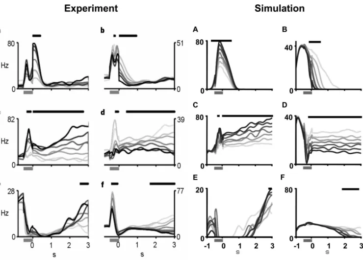
The neural responses (see Fig. 2a–f) have been nominally cat-egorized by their monotonic relationship to the base stimulus, f1 (Romo et al., 1999). Activities that increase with f1 are “positive monotonic,” and those that decrease with f1 are “negative mono-tonic.” Surprisingly, the activities of most neurons are not
persis-tent but display a characteristic ramping up or down behavior. Consequently, the responses are further distinguished by periods of monotonicity. Neurons that are monotonic throughout the delay period are deemed “persistent,” whereas those that are only monotonic during the beginning or end of the delay are desig-nated “early” and “late” neurons, respectively.
In this modeling study, we propose a very simple means of capturing the wide variety of observed responses in a neurally plausible network. The current understanding of working mem-ory is that such areas realize a simple one-dimensional line attrac-tor or a set of such attracattrac-tors (Wang, 1999; Seung et al., 2000; Brody et al., 2003; Miller et al., 2003). Unfortunately, this as-sumption makes it very difficult to capture the wide variety of responses observed by Romo et al. (1999). This was recently dem-onstrated by the model of Miller et al. (2003), in which they were unable to capture responses like those in shown in Figure 2cwith a fairly complex, six-population model. In addition, past models have difficulty incorporating the wide diversity of neural re-sponse functions observed in these areas, usually assuming that any heterogeneity of responses is a result of the “messiness” of neural systems. We demonstrate that by considering a two-dimensional model, all of the categories of responses observed by Romo et al. (1999) can be captured. We show that this is possible only because we explicitly incorporate the heterogeneity ob-served in neural systems into the model. As a result, both the messiness of the system and the higher-dimensional sensitivity of neurons play an important role in explaining the experimental data in a simple, one-population network.
Materials and Methods
To generate and exploit this two-dimensional population, we follow the methodology of Eliasmith and Anderson (2003). Briefly, we begin by randomly choosing neural parameters that fall within biologically
plau-Received Nov. 11, 2005; revised Jan. 23, 2006; accepted Feb. 23, 2006.
This work was supported by grants from the Natural Science and Engineering Research Council (Canada) (261453-03), Canadian Foundation for Innovation (3358401), and Ontario Innovati (3358501). We thank J. Conklin, B. Tripp, and P. Miller for valuable discussions.
Correspondence should be addressed to Dr. Chris Eliasmith at the above address. E-mail: [email protected].
DOI:10.1523/JNEUROSCI.4864-05.2006
sible regimens. We then suggest a plausible population-level encoding and decoding relationship with the relevant stimuli that defines the two-dimensional encoding. Finally, we determine how to instantiate higher-level dynamics (i.e., an appropriate state space trajectory) using this pop-ulation of neurons. The resulting single-cell behavior is then compared with observed data to determine whether the posited encoding, decod-ing, and dynamics are reasonable. Here, we describe each of these steps in detail, with comparisons to more familiar applications to one-dimensional representations.
Central to our results is a general characterization of representation as neural encoding and decoding. The population of neurons in the model is a heterogeneous collection of adapting leaky integrate-and-fire (LIF) neurons. As described in the study by Eliasmith and Anderson (2003), more complex single-neuron models can be used as well, but there is a significant computational cost without much gain in realism, especially in the context of this particular model. The current present in the soma of a particular neuron can be described generically as follows:
Ji共x兲⫽␣i具˜i䡠x典⫹Jibias⫹i, (1) whereJi(x) is the input current to neuroni,xis the vector variable of the stimulus space encoded by the neuron,␣iis a gain factor,˜iis the preferred-direction vector of the neuron in the stimulus space,Jibiasis a bias current that accounts for background activity, andimodels neural noise. Notably, the dot product,具˜i䡠x典, describes the relationship be-tween a high-dimensional physical quantity (e.g., a stimulus) and the resulting scalar signal describing the input current.
For clarity, it is worth comparing the responses of one- and two-dimensional neurons. In the one-two-dimensional case, the preferred-direction vector is either⫹1 or⫺1. Neurons with a preferred direction that is positive are “on” neurons. That is, they will increase their firing rate as the value of the stimulus variable increases. The opposite is true for the negative, or “off,” neurons. The addition of a second dimension generalizes this characterization such that the preferred directions now lie at any direction on the unit circle, rather than just⫾1. Thus, as a constant magnitude stimulus vector sweeps past the preferred-direction vector of the neuron, the firing rate of the neuron will trace out a typical cosine-type tuning curve, with peak firing at the preferred direction. As the magnitude of the stimulus increases at a constant direction (e.g., the preferred direction), the firing rate of the neuron will increase propor-tionally, just as it did in the one-dimensional case (see Fig. 3). In both cases, these tuning curves are, in fact, the result of both Equation 1 and a neural nonlinearity.
In particular, in our model, the time course of the somatic voltage in response to this current evolves as a standard LIF neuron, with the addi-tion of adaptaaddi-tion. These dynamics are captured by (Koch, 1999) as follows:
dVi/dt⫽⫺共Vi共1⫹RGadapt兲⫺Ji共x兲R兲/iRC
dGadapt/dt⫽⫺Gadapt/adapt, (2) whereViis the somatic voltage,Ris the leak resistance,iRCis the RC time constant, andGadaptis the time-varying conductance modulated by
adapt. The system is integrated until the membrane potential,Vi, crosses the neuron threshold,Vth, at which point a␦(t⫺tin) spike is generated,
Gadaptis increased byGinc, andViis reset to zero for the duration of the refractory period,iref. The inclusion of adaptation helps account for the observed effects of stimulus onset (see Fig. 2, gray bars). Notably, includ-ing adaptation does not adversely affect the derivation or overall behav-ior of the model.
As mentioned, it is important for the model to include the heteroge-neity typical of single-cell responses observed in the cortex. Using Equa-tions 1 and 2 as a model of neuron behavior, we randomly select a set of neural parameters. In particular, the preferred-direction vectors,˜i, are drawn from a uniform distribution around the two-dimensional unit circle. The distribution is uniform primarily because we have no indica-tion that it should be otherwise, and this distribuindica-tion has been shown appropriate for other cortical models (Georgopoulos et al., 1984). The gain and bias current,␣iandJibias, are chosen such that the maximum
firing rates are randomly assigned to neurons but evenly distributed between 20 and 100 Hz, to match the data of Romo et al. (1999). The RC time constant is chosen to lie inRC⫽5–15 ms, typical membrane time constant values, and the adaptation constant is set to lie inadapt⫽1–200 ms to reflect the wide variety of adaptation in pyramidal neurons. The refractory period is set toiref⫽1 ms, again a typical value, andGinc⫽20 nS, which has been shown to effectively match cortical adaptation (Koch, 1999). In addition, during the simulation, independent Gaussian noise,
i⫽N(0, 0.1), is injected into the soma to account for various sources of neural noise (e.g., spike jitter, thermal fluctuations, neurotransmitter variations, etc.). In summary, given available evidence, the model popu-lation was closely matched to the parameter regimens that describe the kind of cortical population we suspect Romo et al. (1999) encountered during their recordings. Because many of the parameters are statistically matched, the precise responses of the model population will vary be-tween runs.
We have now completed our characterization of neural encoding (Eqs. 1 and 2). Next we must address how these neurons can use the informa-tion that they have encoded about the stimuli of interest. That is, we must define neural decoding to determine (1) what information regarding the stimulus has been encoded and (2) how the information can be used, transformed, or computed over in a neural circuit.
For each neuron in a neural population, we find a neural decoder,i. This decoder is a least-squares optimal weight that can be applied to the neural activities for estimating the encoded information in the popula-tion (see Appendix, Neural representapopula-tion, for methods used to deter-mine decoders). Together, the elements of Figure 1 show the steps in-volved in encoding and decoding a square wave and a ramp input in a one-dimensional neural population. Specifically, Figure 1bshows the spikes that result from encoding an input signal. Because we have sorted these neurons, and removed adaptation, the encoded information is eas-ily evident in the spike pattern. Figure 1cdepicts example postsynaptic currents (PSCs) that would result in a subsequent population that re-ceives these spikes. This depicts temporally decoded (or filtered) spike trains, an example ofai(t) in Equation 3. Figure 1ademonstrates the results of summing over the population of neurons with such currents and weighting them by their decoders (black line). That is, it shows a decoded estimatexˆ(t) of the original signalx(t). So, the difference be-tween the input and output signals in Figure 1aindicates how well this population has encoded the information in the original signal. To trans-form this encoded intrans-formation (i.e., to compute some function of the input), the same methods can be used to find decoders for each such transformation [see Eliasmith and Anderson (2003) for detailed discus-sion]. This understanding of neural representation generalizes to the dimensional case. Rather than scalar weights, the decoders are two-dimensional vectors, but the methods do not otherwise change.
To this point, we have discussed the two-dimensional representation used in our model. It is this characterization of representation that ex-plains why we are able to produce the variety of results observed in the neural system (see Results). This is because it is the path that the network takes through this representational space that provides an explanation of the data. However, we are also interested in understanding how this path itself is generated. To do so, we need to understand how network-level dynamics can be understood in the context of such representations.
After Eliasmith and Anderson (2003), we assume that the dynamics of the population can be expressed in terms of the dynamics of the signal(s) it is representing. As discussed in detail in the Appendix (see Neural dynamics), taking the neural representation to be the state variable of a dynamic system described by control theory leads to a general method for constructing complex, dynamic neural models. For instance, Elias-mith (2005) provides a comprehensive account of controlled spiking attractor networks (i.e., point, line, ring, plane, cyclic, and chaotic attrac-tor networks) using these methods.
As discussed later, a number of possible dynamic systems can account for the behavior of the working memory neurons of interest here. How-ever, to get a sense of how this variety of dynamics is used to construct a model, let us consider the simple example of a one-dimensional integra-tor. This recurrent network has previously been well characterized (Seung, 1996; Seung et al., 2000; Koulakov et al., 2002; Eliasmith and
Anderson, 2003; Goldman et al., 2003). In summary, to implement a one-dimensional integrator of the signalx, we use our previously defined neural representation ofxto determine the appropriate recurrent con-nection weights. If we would like the population to respectx˙⫽0 [i.e., that there is no change inxover time without input (which defines an inte-grator)], we must ensure that the representation encoded from the neural inputs is the same as the representation decoded from those inputs. Combining Equations 1 and 2, we can write the encoding at the inputs as follows:
ai共t兲⫽Gi关␣i具˜ix共t兲典⫹Jibias兴, (3)
whereGirepresents the encoding defined by Equation 2. We can also write the decoding of this encoded information as a weighted sum (as captured by Fig. 1) as follows:
xˆ共t兲⫽
冘
j⫽1 Naj共t兲j, (4)
whereaj(t) is the neural activity (i.e., the postsynaptic filtered spike trains from neuroni, as shown in Fig. 1c, althoughGiin Eq. 3 should be con-volved with the PSC filter but is left out for simplicity; see Appendix, Neural representation, for a full characterization),Nis the number of neurons in the population, andxˆ(t) is the optimal linear estimate ofx
using the decoders. It should be noted that the subscriptsiandjrange over the same population of neurons, because the connections are recurrent.
With these definitions, we can now construct a one-dimensional neu-ral integrator by allowingxˆ(t)⫽x(t), thus substituting Equation 4 for Equation 3, giving the following:
ai共t兲⫽Gi
冋
␣i冓
˜i冘
j⫽1 N aj共t兲j冔
⫹Jibias册
⫽Gi冋
冘
j⫽1 N ijaj共t兲⫹Jibias册
, (5) whereij⫽␣i具˜ij典. Equation 5 now defines a neural integrator in terms of recurrent connection weights. That is, the circuit with recurrent con-nections that are defined by this weight matrix will have dynamics that are steady (i.e., an unchanging representation) under no input. As de-scribed in the Appendix (see Neural dynamics), this simple derivation can be generalized to arbitrary dynamics and more complex circuits (e.g., with an input signal). As well, it can be generalized to higher dimensions. So, in the two-dimensional case, the preferred-direction (encoding) and decoding vectors replace the encoding and decoding scalars, but other-wise the derivation is the same (see Fig. 6 for plots of these weight structures).
In essence, this derivation is much like those of Seung et al. (2000) and others. They use similar least-squares methods to tune a one-dimensional integrator. However, there are two important differences between past derivations and the one presented here (detailed in the appendices). First, Seung et al. (2000) and others do not characterize the role of the encoders and decoders as we have done. Usually, both are assumed to be free variables for finding the weights. In contrast, we have taken the encoders to be inferable directly from experimentally observed tuning curves. As a result, it is less clear how to generalize past methods to higher dimensions. Here, however, the derivation is the same, regardless of the dimensionality of the tuning curves. Second, we have introduced a general dynamics matrix into our weight derivations, which results in a standard form for the weights ofij⫽␣i具˜
iAⴕj典(see Appendix, Neural dynamics). This is not evident in the simple one-dimensional integrator case, because theAⴕmatrix is equal to 1 and not explicitly included in past derivations. However, as discussed in detail in Results, this characteriza-tion allows us to construct a wide variety of complex dynamics in higher-dimensional spaces.
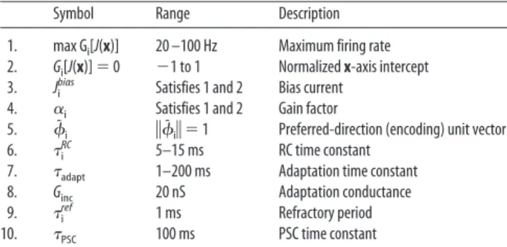
To simulate the data of Romo et al. (1999), circuits derived in this manner were modeled using the Neural Engineering Simulator, which is available as an open source (http://sourceforge.net/projects/nesim). To match the experimental setup of Romo et al. (1999), seven evenly spaced step inputs are used to simulate the base stimulus (f1). The stimulus lasts for 0.5 s, and the delay period runs for 3 s as in the original experiments. The spiking activity of each neuron is collected. Again following the method used by Romo et al. (1999), poststimulus time histogram (PSTH) plots are generated by convolving the spike trains with Gaussian kernels (⫽150 ms during the delay period;⫽50 ms elsewhere). For all simulations, the PSC time constant is 100 ms. A summary of the parameters used can be found in Table 1.
Results
Here, we describe our simulation results and situate them with respect to past attempts at modeling the observed working
mem-Figure 1. Population encoding and decoding of a square pulse and ramp signal.a, The input
x(t) (gray line) and the decoded estimate,xˆ(t) (black line), using a population of 100 one-dimensional LIF neurons. The weighted sum all of the PSCs yields the decoded estimate (black line).b, The spike raster produced by encoding the input. Neurons are separated ati⫽50 into on and off neurons ( ˜i⫽⫹1 and⫺1, respectively) and sorted by firing onset.c, The rasters of
neuronsi⫽80, 50, and 35 are plotted with their resulting PSCs. Notably, these were chosen to hint at the ramping response of early, persistent, and late firing seen in the data of Romo et al. (1999).
ory effects. We then provide a taxonomy of network topologies that give rise to the dynamics needed to explain the data of Romo et al. (1999).
Related work
Much effort has been spent designing systems that maintain a persistent signal after stimulus presentation, the presumed pur-pose of working memory. However, this approach is somewhat at odds with the data, which suggests that the majority of working memory signals are not persistent. Hence, our purpose here is to describe a neural model that reproduces the dynamics of the data of Romo et al. (1999). We are less concerned with neural mech-anisms for signal persistence (Seung, 1996; Koulakov et al., 2002; Goldman et al., 2003). Nevertheless, as described above, our so-lution is related to that of Seung et al. (2000), and we provide some discussion of the robustness of the solution to fine-tuning and noise. However, here we address the more immediate ques-tion: How can memory be reliably encoded in a time-varying signal and what explains the wide variety of dynamics observed in working memory?
Miller et al. (2003) have recently proposed a model that ad-dresses this question directly, and in the context of the vibrotac-tile discrimination task. Their model consists of a large network of LIF neurons in a locally structured circuit. To avoid the fine-tuning problem that plagues some neural integrators [like that of Seung et al. (2000)], Miller et al. (2003) use a collection of bistable groups to create a network of multi-stable states (Koulakov et al., 2002). However, they conclude that non-finely tuned networks do not properly reflect the data because such networks result in highly discontinuous neuron responses. Additionally, they dem-onstrate that fine tuning is a reasonable alternative, which is also supported by our results below.
Of greater interest here is how they attempt to reproduce the wide variety of observed neural dynamics. To do so, they propose a network of three neural integrator populations that capture the characteristic ramping up, down, and tonic behaviors. The pop-ulations are assumed to be assembled together with suitable ex-citatory and inhibitory connections. Each population consists of two subnetworks: one that supports negative monotonicity and one that supports positive monotonicity. Each subnetwork con-sists of 12 neuronal groups of 500 neurons each (the bistable integrators). The resulting subnetworks have 6000 neurons each for a total of 36,000 in the entire network (although each popu-lation of 12,000 neurons is simulated independently).
Although their model can broadly simulate the categorized responses, it is unable to reproduce the wide variety of neural responses seen in data set of Romo et al. (1999). For instance, neurons in the study by Miller et al. (2003) exhibit either tonic or ramping curves but not variations of both, as in Figure 2,candC,
where the high-frequency responses are ramping but the low-frequency responses are tonic. This is because, like other past characterizations of working memory (Zipser et al., 1993; Cam-peri and Wang, 1998; Reutimann et al., 2004), Miller et al. (2003) tacitly assume that neural responses in their populations encode only one-dimensional signals. As a result, monotonicity with re-spect to frequency is rendered independent from time-varying dynamics. These features are then further subdivided: monoto-nicity is split into positive and negative monotonic neurons, and time-varying dynamics are split into ramping up or down ten-dencies. Unfortunately, this divide-and-conquer approach has two limitations. First, it unnecessarily complicates matters. For instance, there is no need to explicitly simulate two oppositely ramping responses; using a two-dimensional population with randomly distributed preferred directions in the two-dimensional space automatically provides neurons with oppo-sitely directed tuning curves that naturally account for this kind of behavior. Second, it results in missing some of the observed properties of neural tuning. In addition to not reproducing Fig-ure 2,candC, separating the two dimensions will result in ramp-ing neurons always startramp-ing from an initial (background) posi-tion and “fanning” outward, although the opposite (fanning inward) is seen in Figure 2,aandA.
Simulation results
The empirical responses shown in Figure 2a–f clearly portray neurons that are both time and stimulus dependent. These de-pendencies are independent only in the sense that frequency monotonicity does not dictate time-varying behavior. This does not entail that the representation of these dimensions needs to be independent, however. Thus, we propose a model that views neu-rons as simultaneously sensitive to both quantities, with those sensitivities evenly and randomly distributed in a two-dimensional space (see Materials and Methods). In particular, we assume that the two-dimensional space of interest has, as its di-mensions, “time” (i.e., a representation of time; but see Discus-sion) and frequency. Mathematically, we denote the two quanti-ties as the parameterized vectorx(t)⫽[F(t),T(t)] (Fig. 3). Let us first consider the role of this representation in explaining the data of Romo et al. (1999).
Neurons representing this space will maximally fire to some “preferred stimulus,” which defines a direction in the two-dimensional space as depicted in Figure 3. As a result, the ob-served gradations in sensitivity in a particular direction should be a reflection of the heterogeneity of intrinsic neural response curves (where such curves are understood as the responses found by direct current injection). So, a representation of the two-dimensional space that consists of randomly distributed pre-ferred directions, along with a variety of intrinsic neural response curves, should correspond to the different kinds of tuning shown in Figure 2. Notably, these curves have been selectively chosen to match the experimental data. It would be more informative to compare the entire distribution of tuning curves to determine how typical such neuron classes are. However, because we were unable to examine the complete original data set, we cannot affect this comparison. The even distribution that we have assumed for tuning curves results in a wide variety of responses, many of which are intermediate between the classes shown in Figure 2. Other distributions would result in more “clustered” preferred-direction vectors and thus fewer and more typical cell classes. Given the general tendency to observe high heterogeneity in the cortex, we take the even distribution to be a reasonable assumption.
Table 1. Model parameters
Symbol Range Description 1. max Gi[J(x)] 20 –100 Hz Maximum firing rate
2. Gi[J(x)]⫽0 ⫺1 to 1 Normalizedx-axis intercept
3. Ji
bias Satisfies 1 and 2 Bias current
4. ␣i Satisfies 1 and 2 Gain factor
5. ˜i 储˜i储⫽1 Preferred-direction (encoding) unit vector 6. i
RC 5–15 ms RC time constant
7. adapt 1–200 ms Adaptation time constant
8. Ginc 20 nS Adaptation conductance
9. i
ref 1 ms Refractory period
However, this characterization of the neural representation alone does not account for the changes over time of the neural responses. The specific values taken on by the two-dimensional quantity through time (i.e., the state space trajectory or dynam-ics) also play a significant role. Assuming a two-dimensional rep-resentation that consists of a time and frequency dimension, as
we have, examination of the experiments of Romo et al. (1999) suggests that the observed dynamics result from a combination of a constant signal along the frequency dimension (the memory of f1) and a ramping signal in the time dimension.
To test this account, we built and simulated a network of two-dimensional neurons that realized this trajectory (see Mate-rials and Methods). The results are plotted in Figure 2A–Fand are juxtaposed with the experimental findings. The simulation reveals early, late, and persistent neurons that exhibit positive and negative monotonic responses, all of the classes of response de-scribed in the original data. So, the model demonstrates that the observed PSTHs can be understood as primarily the result of two-dimensional neural tuning curves and the dynamics of a two-dimensional quantity. Figure 4 provides a geometric expla-nation of how dynamics and tuning curves interact to result in the observed responses. In Figure 4b, filtered spike trains are shown as a function of the state space trajectory projected onto the two-dimensional tuning curve of a neuron. The path traveled on this surface is driven by the dynamics of the working memory signal. Each set of input signals produces a characteristic and systematic path across the surface. We can thus understand the observed variety of responses in the experiments: the PSTHs vary systematically with f1, yet generally maintain the same shape be-cause there is a monotonically increasing time signal,T(t), over a consistent (neural) nonlinearity.
The variety of observed tuning curves is thus explained by the
Figure 2. PSTH plots during memorization. The gray bars under the axes indicate the onset of the stimulus, and black bars above the graph mark periods of monotonicity. The higher stimulus frequency (f1) is marked with darker response curves.a,c,e, Positive monotonic.b,d,f, Negative monotonic.a,b, Early neurons.c,d, Persistent neurons.e,f, Late neurons. [Data are from Romo et al. (1999).]A–F, Corresponding simulation results from the model shown.
Figure 3. Tuning curve of a two-dimensional neuron defined byGi[␣i具˜i䡠X典 ⫹Ji bias. For
this neuron, the preferred-direction vector is ˜i⫽[⫺0.64, 0.766]. Three state space
trajecto-ries, defined byx(t)⫽[F(t),T(t)], are shown projected onto the curve. For each trajectory,F(t) is a constant,T(t) is a ramping signal, andtranges from 0 to 3 s. The units ofF(t) andT(t) are open to interpretation, but one can view them as normalized frequency and time, respectively.
distribution of preferred-direction vectors,˜⫽[˜f,˜t], the firing
thresholds (along those vectors) in the two-dimensional space, and the neural nonlinearity. Generally, monotonicity is deter-mined bysign(˜f), and early, late, and persistent firing is
charac-terized by˜t. As mentioned, we chose the vectors randomly from
an even distribution over the unit circle and the response thresh-old randomly from an even distribution along the vector. Better fits to the likelihoods of observing various classes of responses could be made by altering these distributions to match the neural data (the complete data set was not available).
The key difference between this model and that of Miller et al. (2003) is in the representation of the content of memory. Rather than taking neurons to encode a series of one-dimensional sig-nals, we understand them to encode a single two-dimensional space. As a result, the myriad of observed responses are a natural consequence of a heterogeneous population of individual neuron tuning curves directed in this higher-dimensional space. As a result, Figure 2,candC, is observed in our model but not in that of Miller et al. (2003). Additionally, this approach results in a much more efficient use of neural resources. The results pre-sented in Figure 2 are from a network of⬍3000 neurons (the organization of which is described below). This is an order of
magnitude fewer neurons than in the model of Miller et al. (2003), despite a more complete characterization of the observed data, and the same degree of dynamic stability.
It is worth emphasizing that the neurons in our model are, biophysically speaking, no different than those in past models. The important difference is in how we have characterized what those biophysical states are used to represent. As a result, refer-ring to these neurons as higher dimensional denotes the fact that they are sensitive to multiple physical dimensions concurrently. This, it should be noted, has nothing to do with the dimension-ality of the equations used to describe the time course of the voltages and currents in the neuron model itself. What these results show, then, is that mapping biophysical states of cells into higher-dimensional representational spaces can more effectively explain the observed transitions between those biophysical states in real neural systems.
Dynamics
Our discussion so far leaves unresolved why or how this popula-tion has the particular trajectory through the state space that it does (i.e., a coupled ramp and constant). We address these ques-tions in detail here. Systematically characterizing network-level dynamics is essential because the time-varying activity might be explained by a number of competing hypotheses. Some have sug-gested that the network encodes the passage of time, which could be used to deduce f1 (Brody et al., 2003; Reutimann et al., 2004). Others have posited that signals with the necessary time course are broadly projected to the PFC (Fiorillo et al., 2003). These latter signals are thought to encode reward uncertainty and could account for the observed dynamics in the PFC neurons. For the most part, our modeling effort is agnostic as to the exact nature of this quantity. However, here we discuss and model the architec-tural implications of these different kinds of explanations for the observed dynamics.
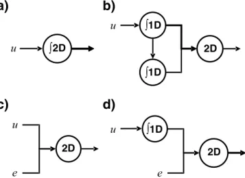
Recall that we have identified the necessary state space trajec-tory as including a constant signal related to f1 and a time-varying ramp signal, time. Clearly, then, any network architecture that results in this state space trajectory will give rise to the single-cell responses depicted in Figure 2. Figure 5 depicts four network topologies that result in this trajectory. The topologies can be
Figure 4. a, Response curves of a late positive monotonic neuron.b, The spiking rates can be seen as a mapping of the state space trajectory onto the two-dimensional tuning curve of the neuron. The trajectories of every other curve inaare shown. The responses do not lie exactly on the curve (as in Fig. 3) because of accumulated noise.
Figure 5. Network architectures that produce the observed responses.a, A simple two-dimensional integrator.b, Coupled one-dimensional integrators.c, Projected external signals.
d, One-dimensional integrator with an external input. The circuits can be categorized as either using two-dimensional integration (a,c) or two-dimensional projection (b,d) with inputs that are locally generated (a,b) or external (c,d). 2D, Two-dimensional; 1D, one-dimensional.
categorized as either using purely two-dimensional representa-tions (Fig. 5a,c) or not (Fig. 5b,d), with behavior that is either entirely locally generated (Fig. 5a,b) or not (Fig. 5c,d). Note that all networks eventually rely on a two-dimensional representation to explain the results. We believe that this taxonomy of networks can both guide and be adjudicated by experimental results, as discussed. First, however, we turn to a brief characterization of each topology.
Two-dimensional integrator
Neural integration is a robust and common phenomenon across brain areas and has been widely associated with working memory (Douglas et al., 1995; Seung, 1996, 2000; Aksay, 2000, 2001). Because we are using a two-dimensional representation, it may make sense to account for this phenomena using a local, two-dimensional integrator.
In terms of the desired trajectory through the two-dimensional space, one dimension of the signal must represent the frequency,F(t), and the other must represent a monotoni-cally increasing function of time,T(t), that is dependent on the initial frequency.F(t) can be linked directly to the integration of f1, whereasT(t) can be considered an integration of the inte-grated f1 signal. In other words, to reproduce the observed re-sponse curves, we must integrate both the input frequency (to remember it) and the results of that integration (to generate the ramping time signal).
These “double-integration” dynamics can be defined in stan-dard control theoretic terms, using the dynamics equation, x˙(t)⫽Ax(t)⫹Bu(t), as follows:
冋
x˙1 x˙2册
⫽冋
0 0 ␣ 0册冋
x1 x2册
⫹冋
1 0 0 0册冋
u 0册
, (6) whereurepresents the stimulus presentation and␣is a constant that scales the effect of the frequency component on the time component (i.e., the second integration). As described in the Appendix (see Neural dynamics), we can use Equation 13 to con-vert this two-dimensional integration network into a neurally implementable network:A⬘⫽
冋
␣1 01册
,B⬘⫽冋
0 00册
. (7) As described in Results, this is a natural extension of previous characterizations of a one-dimensional integrator. The difference lies in the fact that the representation is two-dimensional and the dynamics are slightly more sophisticated, as reflected in the dy-namics matrixAⴕ.In our simulations of up to 3000 neurons, this circuit is un-stable, because trajectories drift rapidly and then rest on one of a few attractor points (data not shown). These problems can be alleviated with longer time constants (which may be biophysi-cally unrealistic), by adding neurons (Eliasmith and Anderson, 2003) (we were unable to pursue this solution further because of computational limitations), by including more sophisticated control circuits (e.g., a differentiating compensator), or by intro-ducing varieties of hysteresis (Koulakov et al., 2002; Goldman et al., 2003).
Coupled one-dimensional integrators
Alternatively, it is possible to implement a similar solution in which the integration dynamics are handled in separate popula-tions. Figure 5bshows the topology of such a network. Here, two one-dimensional integrators implement the same dynamic sys-tem (i.e., double integration) and project their results into a
two-dimensional population. Nevertheless, Equation 6 describes the dynamics of this network as well, because only the representation and not the dynamics have changed. More accurately, Equation 6 could be written as two separate coupled differential equations (although this is mathematically equivalent). The reason two dif-ferent architectures are described by the same equations is be-cause anatomical constraints are important for determining the precise relationship between a dynamical description and its im-plementation in a set of neurons, although such constraints are not capture by the equations. So, the difference between panelsa andbin Fig. 5 is the result of a difference in our assumptions regarding anatomical organization in these two cases (in the first that there are broad reciprocal projections from all two-dimensional neurons, in the second that there are feedforward projections from the one-dimensional integrators to the two-dimensional population).
The results from this network are shown in Figure 2A–F. To achieve these results, each integrator used 1000 one-dimensional neurons, and the two-dimensional population consisted of 500 neurons. The network is highly stable and thus able to reproduce the results from the experiment. Notably, both this solution and the previous one assume that the signals driving the movement through the two-dimensional state space are internally gener-ated, which is consistent with the idea that the network itself is keeping track of the time elapsed between stimulus presentations. Projected external signals
Unlike the characterization of the previous two architectures, the dynamics could be driven by external signal sources. For in-stance, signals from the ventral tegmental area project to the PFC and could account for the time-varying signal observed in work-ing memory. However, the existence of rampwork-ing signals seem to be sensitive to the uncertainty regarding a reward, whereas the monkey in these experiments receive a reward on almost all trials. Indeed, it is possible that both theF(t) andT(t) signals are exter-nal to the population in the PFC. In this scenario “working mem-ory” is a misnomer for the function of this area, because there is no active maintenance of a local signal in the region. Rather, the PFC would simply be a merging of two independent signals into a single two-dimensional representation. The results from this network are identical to those presented in Figure 2, given appro-priate input signals.
Including such external signals can be accomplished with a simple modification of Equation 6:
冋
x˙1 x˙2册
⫽冋
␣1 0 0 ␣2册冋
x1 x2册
⫹冋
1 0 0 1册冋
u e册
. (8) With␣1,2⬍0, neither dimension will be integrated as it was in theprevious networks and will thus both reflect the external signals directly.
One-dimensional integrator with one external input
If, however,␣1⫽0 or␣2⫽0, then the corresponding dimension
will be integrated. Thus if only the frequency or time signals were projected into the network from an external source, appropri-ately varying Equation 8 will reflect this fact. For instance, sup-posing that␣1⫽0, thenuwould reflect the standard input to
working memory that would be integrated in this area, ande would reflect an externally generated ramping time signal. The results of simulating this network are identical to those in Figure 2 given appropriately chosen external signals for the chosen dynamics.
General dynamics results
Despite this variety of possible architectures, there are some gen-eral insights that can be gained from examining them together (we discuss ways of empirically distinguishing these topologies in the Discussion). First, it is useful to recall at this point that the connection matrices for all dynamics in these various architec-tures are of the same form (i.e.,ij⫽␣1具˜iAⴕjx典for recurrent
connections andij⫽␣1具˜iBⴕku典for input connections).
Obvi-ously, the specific values of these variables will change the precise structure of the matrices. Nevertheless, there is some degree of “typical” structure for recurrently connected integrators, regard-less of their dimension (Fig. 6a,b). Specifically, both one- and two-dimensional integrator populations display a noisy center-surround organization, although this pattern is more evident in the two-dimensional case. For the one-dimensional case, there are only two possible encoders (⫾1), so the diagonal center is the size of half of the population. However, this center-surround structure has been observed in higher dimensions (e.g., 25 di-mensions) as well (Conklin and Eliasmith, 2005). And this pat-tern is strikingly similar to the hand-constructed center-surround weight matrices used in past integrator models (Zhang, 1999). As a result, if connectivity patterns of neural populations
resemble this general pattern, they may be involved in a form of neural integration for any dimensionality of representation.
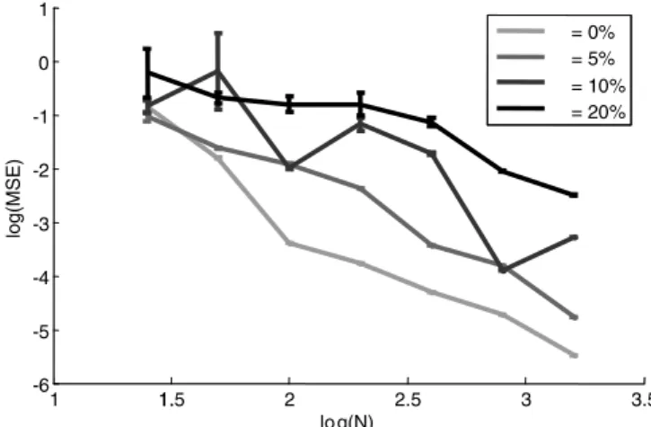
One concern that arises with constructing weight matrices using these methods is the “fine-tuning problem” (i.e., the prob-lem of making the matrix robust to noise). One difficulty with this characterization of the problem is that whether or not there is actually a problem depends on the precise kind of disturbance introduced. The weights in these networks are clearly robust to some noise, as demonstrated by Figure 7. This figure shows that a desired mean squared error (MSE) can be reached by increasing the size of the integration population. Specifically, it can be seen that the effects of the noise go down as⬃1/N. These results indi-cate that the integrator will be robust even for small population sizes, because integrator stability is directly related to the MSE (Eliasmith and Anderson, 2003). Similar robustness results for a high-dimensional integrator have been reported by Conklin and Eliasmith (2005), who showed that integration behavior was only mildly affected by the addition of up to⫽50% noise.
However, this robustness is to zero mean, independent Gauss-ian noise. We have no reason to believe that our network will be especially robust to non-zero mean noise in the connection weights. What is of importance, then, is not the presence of noise, but rather some population-wide bias (e.g., shifting all weights in one direction). We are unaware of any experimental results indi-cating that such biases should be expected here, or in any other integrator networks. We suggest that fine-tuning is thus a misno-mer for the problem (because we can add random noise the weights to a large degree and the network still functions). Perhaps it should be called the “biased weight problem” instead.
Discussion
There are three major insights to be drawn from these results. First, a two-dimensional neural representation can underwrite a natural, efficient, and robust network that explains the wide va-riety of responses exhibited by working memory neurons. In this regard, it is important to note that this approach is also relevant for systems with nonmonotonic (e.g., peaked) tuning curves, which are observed in many working memory tasks (Nieder et al., 2002). This is because if the dimensions of the representation are polar coordinates (rather than Cartesian), peaked tuning natu-rally results (because a sweep around thedimension produces a
Figure 6. Recurrent connection weights for the one-dimensional integrator (a) and two-dimensional integrator (b). Both axes areN, the neuron number assigned after sorting the neurons by their encoders and decoders. The depth of gray indicates connection strength. These matrices demonstrate the systematic relationship between center-surround connectivity and attractor networks of any dimension.
Figure 7. Network robustness to connection weight noise. This is a log–log plot of the MSE as a function of the number of neurons (N) and the amount of Gaussian noise added to the weights in the connection matrix. The noise added is calculated by taking the indicated percent-age as the SD of Gaussian, independent mean zero noise that is then scaled by the original size of the weight.
peak centered on the preferred-direction vector), and the dynam-ics can be described analogously. Notably, higher-dimensional models can also result in this kind of peaked tuning (Eliasmith and Anderson, 2003; Conklin and Eliasmith, 2005). These repre-sentations may be relevant for understanding working memory in visual areas, which are sensitive to a large number of dimensions.
Second, this explanation relies on the observed heterogeneity of neural responses. Elsewhere, we have argued that neural het-erogeneity is a natural result of a trade off between representa-tional efficiency and simple organizarepresenta-tional mechanisms in neural systems (Eliasmith and Anderson, 2003). So, this work supports the idea that, rather than being a sign of the intractability of neural systems, heterogeneity is both consistent with efficient neural computation and essential to incorporate into models at-tempting to explain such computation.
Third, these results provide evidence that the methods used here allow for effective, plausible, and quantitative characteriza-tions of neural representation and neural dynamics resulting from a wide variety of possible network topologies.
However, these conclusions do not directly address two cen-tral empirical questions: (1) How might we tell whether working memory uses a two-dimensional rather than one-dimensional (or higher-dimensional) representation? (2) How can we adjudi-cate between the possible network topologies that give rise to the state space trajectory?
Regarding the first question, we note that one benefit of a two-dimensional representation is that it supports the linear ex-traction of nonlinear functions of the represented dimensions (Eliasmith and Anderson, 2003). If these neurons are used to encode not only stimulus parameters but also act as a kind of preparatory signal [as suggested by Brody et al. (2003)], extract-ing such a function is essential. So, the model leads to the predic-tion that some neural populapredic-tions that receive projecpredic-tions from this area will compute nonlinear functions of the represented variables (which should be evident in their tuning). This high-lights the close link between nonlinear computation and higher-dimensional representation (under the assumption that neural populations in the cortex perform linear transformations, i.e., by summing weighted synaptic input).
However, this does not address the question of whether the population may be representing more than two dimensions. This is a valid concern because our simulation does not display all of the subtleties of the data. For example, the minor ramping of early neurons after the first second (Fig. 2a,b) are absent in our simulations (Fig. 2A,B). Additionally, we do not find the “down-then-up” responses evident in some neurons (data not shown). Despite the fact that these responses account for a small portion of the categorized curves, higher-dimensional extensions to the current model might account for these additional phenomena. A principal, or independent, component analysis of the experimen-tal data could provide a good indication of how many dimensions are required. It is important to note, however, that such features of the data might also arise from different dynamics: including the state space trajectory (we have assumed a very simple one).
Considering the number of dimensions needed to model the data highlights predictions that distinguish models of different dimensions. From a purely mathematical point of view, any D-dimensional representation can be reproduced by D one-dimensional representations (because both representations span the D-dimensional space). However, when there are resource constraints (e.g., maximum firing rates), these two representa-tions can be distinguished because saturation effects will be
dif-ferent. Consider two two-dimensional populations: the first has all preferred-direction vectors aligned with thex-ory-axes (be-cause it is equivalent to two one-dimensional populations, we call it the one-dimensional model), and the second has preferred-direction vectors evenly distributed over the two-dimensional space (the two-dimensional model). Distributions between these two extremes will show related effects to greater and lesser de-grees. In the first case, the saturation of representations along the xdimension will be unaffected by any variations in the represen-tations along theydimension. In the second case, for the majority of preferred-direction vectors, any increase in x-related firing results in a comparable reduction in the range ofydimension values that can be represented before saturation. These effects will likely only be observed for delay periods longer than the expected delay because of rapid renormalization of the stimuli. If the renormalization is rapid enough, it may only be the first trial after that expectation is violated that shows the effects. These effects should be both neurally and behaviorally observable.
Consider high-frequency trials and neurons with positive monotic, downward ramping responses. In the two-dimensional model, such neurons are nearly saturated by the frequency input but are driven toward zero by the ramping time signal. This sets up a conflict between the representation of frequency and time. So, after the saturation of the time signal (i.e., in which the time signal is very negative for the neurons), these neurons will never-theless have an above background firing rate because they are also contributing to the representation of frequency. As a result, they will downward slope but level off, even with an increasing time signal. In contrast, a one-dimensional model will have all down-ward ramping neurons driven to very low or zero firing rates. This is because they are only representing the temporal aspect of the signal, so there is no source of current (e.g., from representing frequency) to counteract the strong downward signal.
Behaviorally there should be differences as well. In the trials that violate the expected delay period, there should be a progres-sive worsening of accuracy of response as the time course goes past the expected delay period, because thexandydimensions interact, andyis ramping. However, this accuracy effect should level off once both dimensions are saturated. In contrast, in a one-dimensional model, there should be no effect on accuracy of changes in time delay, because the dimensions represent (and therefore saturate) independently.
Turning to the second question (adjudication of network dy-namics), distinguishing these network topologies could be ac-complished through carefully constructed microstimulation ex-periments. This methodology has been applied to work in decision making, motion processing, eye control, and tactile working memory (Cohen and Newsome, 2004). Although there are some concerns regarding the application and effects of stim-ulation, the ability of microstimulation to elicit equivalent re-sponses to tactile stimuli in S1 (Romo et al., 1998) suggests the somatosensory cortex may be a good target for microstimulation. As well, microstimulation has been applied successfully to char-acterizing neural integration, a closely related form of dynamics (Kustov and Robinson, 1995).
Microstimulation could be highly informative regarding the network topology both for distinguishing the origin of the sig-nals, and for distinguishing one- and two-dimensional integra-tion. In the first case, if the memory signal is not stored in this anatomical area but rather is projected to the network, brief stim-ulation should only temporarily affect the representation during the delay period. If, however, stimulation resulted in disruption of the dynamics, and hence performance on the task, then the
signals are at least partially locally generated. The differential effects of microstimulation on one- or two-dimensional integra-tors is likely more subtle. If both signals are disrupted after stim-ulation and there is a systematic relationship between the two disruptions (e.g., the time signal is still the integral of the fre-quency signal), then Figure 5bis most likely. In contrast, if both signals are arbitrarily disrupted by stimulation, Figure 5ais more likely because the representation and dynamics in both dimen-sions will be changed concurrently. If only one or the other signal is locally generated, then only that signal would be disrupted by microstimulation. So, it would be difficult to distinguish panelb from paneldin Figure 5, because both are consistent with that outcome. Thus, a series of results in which either the time signal is disrupted or both signals are disrupted would be required to make Figure 5bmore likely. If only one of the signals was ever disrupted, then Figure 5dis more likely. We should note that this reasoning is dependent on the assumption of very small back-propagation effects during microstimulation. It is commonly as-sumed that microstimulation is highly local, affecting an area of only⬃200m or a few hundred cells (Tu and Keating, 2000; Cohen and Newsome, 2004). However, some studies suggest the possibility that the effects could traverse hemispheres (Seide-mann et al., 2002).
In conclusion, our simulations demonstrate that a diverse population of two-dimensional neurons can naturally reproduce the data of Romo et al. (1999). We have emphasized how the methods exploited here can suggest ways of systematically ex-ploring the possible topologies to generate these results. Doing so makes it clear that limiting models to one-dimensional represen-tations unnecessarily limits the hypotheses being considered and can overcomplicate models of the observed responses. Given general methods for building models with higher-dimensional populations, and given the availability of data that are highly suggestive of trajectories through higher-dimensional spaces, there is good reason to adopt this kind of alternative explanation of neural behavior.
Appendix
Neural representation
We take representation in neural populations to be characterized in terms of a nonlinear encoding process and a linear decoding process (Eliasmith and Anderson, 2003). Encoding involves con-verting a quantity,x(t), into a spike train:
冘
n ␦共t⫺tin兲⫽Gi关Ji共x共t兲兲兴, (9)whereGi[䡠] is the nonlinear function describing the spiking
re-sponse (see Figs. 3 and 4bfor typical LIF responses), Jiis the
current in the soma of the cell,iindexes the neuron, andnindexes the spikes produced by the neuron. Note that the driving current is described in detail by Equation 1 and the nonlinearity is de-scribed by Equation 2. Equation 9 captures the nonlinear encod-ing process from a high-dimensional variable, x, to a one-dimensional soma current,Ji, to a train of spikes,␦(t⫺tin).
To understand how a neural system might use the informa-tion encoded into a spike train in this manner, we must charac-terize a neurally plausible decoding as well. To do so, we need to understand how this information can be converted from spike trains back into a relevant quantity. Note that we are not suggest-ing that this decodsuggest-ing process takes place explicitly in neurons. Rather, it is a theoretically useful means of characterizing part of the information processing characteristics of neurons. In partic-ular, we characterize decoding in terms of PSCs and connection
weights. Somewhat surprisingly, a plausible means of character-izing this decoding is as a linear transformation of the spike train. Specifically, we can estimate the original stimulus vectorx(t) by decoding an estimate,xˆ(t), using a linear combination of filters, hi(t), weighted by decoding weights,i, as follows:
xˆ共t兲⫽
冘
in
␦共t⫺tin兲*hi共t兲i⫽
冘
inhi共t⫺tin兲i, (10)
where * indicates convolution (see Fig. 1). Thesehi(t) are thus
linear decoding filters that, for reasons of biological plausibility, we take to be the PSCs in the subsequent neuron.
Revisiting Figure 1, we can understand the depicted processes in terms of these equations. The encoding in Figure 1bproduces a raster of spike trains,␦(t⫺tin), wheretinindicates thenth spike
for neuroni. Neurons are separated ati⫽50 into on and off neurons (˜i⫽ ⫹1 and⫺1, respectively) and sorted by firing
onset (the value ofxfor whichGi[Ji(x)]⫽0). In Figure 1c, spike
trains are plotted with their PSC-filtered counterpart [i.e., hi(t⫺
tin)⫽␦(t⫺tin) * hi(t)]. Finally, the weighted sum of all of the
filtered trains,⌺inhi(t⫺tin)i, yields the overall decoded estimate
(Fig. 1a, black line).
To find theiweights to determine this estimate, we minimize
the mean-squared error (see also Salinas and Abbott, 1994; Seung et al., 2000): E⫽1 2具关x共t兲⫺xˆ共t兲兴 2典 x,t ⫽12具关x共t兲⫺
冘
in 共hi共t⫺tin兲⫹i兲i兴2典x,t, (11)where具䡠典xdenotes integration over the range ofxandimodels
the expected noise. By optimizing with Gaussian random noise, we ensure that fine tuning is not a concern, because the decoding weights will be robust to fluctuations.
This method provides a means of definingn-dimensional rep-resentations in a biologically plausible population of neurons. Here, we have taken the population,i, and temporal,hi(t),
de-coders to be independent, although this is not necessary, as can be seen from the fact that Equation 11 can also be minimized over time.
Neural dynamics
For generality, we can write the relevant dynamics of a popula-tion in a control theoretic form (i.e., using the dynamics state equation that comprises the foundation of modern control theory):
x˙共t兲⫽Ax共t兲⫹Bu共t兲, (12) whereAis the dynamics matrix,Bis the input matrix,u(t) is the input or control vector, andx(t) is the state vector (see Fig. 8afor a graphical depiction of this equation). In general, these matrices and vectors can describe a wide variety of linear, time-invariant physical systems [Eliasmith and Anderson (2003) show how these same methods apply to time-varying and nonlinear systems as well]. Here, we use Equation 12 to capture the hypothesized high-level dynamics of a population of neurons.
Initially, this high-level characterization is divorced from neural-level, implementational considerations. However, it is possible to modify these matrices to render the system neurally plausible. First, we must account for intrinsic neural dynamics by converting this characterization into a neurally relevant one (Fig.
8b). To do so, we assume a model of PSCs given by h(t) ⫽ ⫺1e⫺t/and can derive the following relationship between
pan-elsaandbin Figure 8 [see Eliasmith and Anderson (2003) for a discussion that justifies assuming this (or, more generally, any typically “peaked”) PSC model]:
A⬘⫽A⫹I.
B⬘⫽B (13)
So, our description of the high-level neurally plausible dynamics becomes the following:
x共t兲⫽h共t兲*关Aⴕx共t兲⫹Bⴕu共t兲兴. (14) Notably, this transformation is general and assumes nothing about the form ofAorB. So, given any behavioral system defined in the form of Equation 12, it is possible to construct the neural counterpart by solving forAⴕandBⴕ. A variety of applications of this method to linear, nonlinear, and time-varying neural sys-tems is described by Eliasmith (2005).
Next, we must incorporate this high-level description of the dynamics with our previous characterization of the neural repre-sentation. To do so, we combine the dynamics of Equation 14, the encoding of Equation 9, and the population decoding ofxandu from Equation 10. That is, we takexˆ⫽ ⌺jnhj(t⫺tjn)jxanduˆ⫽
⌺knhk(t⫺tkn)ku, which gives the following:
冘
n ␦共t⫺tin兲⫽Gi关␣i具˜ix共t兲典⫹Jibias兴⫽Gi关␣i具˜i关Aⴕxˆ共t兲⫹Bⴕuˆ共t兲兴典⫹Jibias兴
⫽Gi关␣i具˜i关A⬘⌺jnhj共t⫺tjn兲jx⫹Bⴕ⌺knhk共t⫺tkn兲ku兴典⫹Jibias兴.
(15)
It is important to keep in mind that the temporal filtering is only done once (here included in the estimate of the signals), despite the fact that it is include in both Equations 14 and 10. That is,h(t) in these equations both defines the dynamics and defines the decoding of the representations. To put it in a more familiar form, this equation can be written as follows:
Gi关␣i具˜i关Aⴕ⌺jnhj共t⫺tjn兲jx⫹Bⴕ⌺knhk共t⫺tkn兲ku兴典⫹Jibias兴
⫽Gi关⌺jnijhj共t⫺tjn兲⫹⌺knikhk共t⫺tkn兲⫹Jibias兴, (16)
whereij⫽␣1具˜iAⴕjx典andik⫽␣1具˜iBⴕku典are the recurrent
and input connection weights, respectively. These weights will now implement the dynamics defined by the control theoretic structure from Equation 14 in a neurally plausible network.
References
Aksay E, Baker R, Seung HS, Tank DW (2000) Anatomy and discharge properties of pre-motor neurons in the goldfish medulla that have eye-position signals during fixations. J Neurophysiol 84:1035–1049. Aksay E, Gamkrelidze G, Seung HS, Baker R, Tank DW (2001) In vivo
in-tracellular recording and perturbation of persistent activity in a neural integrator. Nat Neurosci 4:184 –193.
Brody CD, Romo R, Kepecs A (2003) Basic mechanisms for graded persis-tent activity: discrete attractors, continuous attractors, and dynamic rep-resentations. Cogn Neurosci 13:204 –211.
Camperi M, Wang X-J (1998) A model of visuospatial short-term memory in prefrontal cortex: cellular bistability and recurrent network. J Comput Neurosci 5:383– 405.
Cohen MR, Newsome WT (2004) What electrical microstimulation has re-vealed about the neural basis of cognition. Curr Opin Neurobiol 14:1–9. Conklin J, Eliasmith C (2005) An attractor network model of path
integra-tion in the rat. J Comp Neurosci 18:183–203.
Douglas R, Koch C, Mahowald M, Martin K, Suarez H (1995) Recurrent excitation in neocortical circuits. Science 269:981–985.
Eliasmith C (2005) A unified approach to building and controlling spiking attractor networks. Neural Comp 17:1276 –1314.
Eliasmith C, Anderson C (2003) Neural engineering: computation, repre-sentation, and dynamics in neurobiological systems. Cambridge, MA: MIT.
Fiorillo CD, Tobler PN, Schultz W (2003) Discrete coding of reward prob-ability and uncertainty by dopamine neurons. Science 299:1898 –1902. Funahashi S, Bruce CJ, Goldman-Rakic PS (1989) Mnemonic coding of
vi-sual space in the monkey’s dorsolateral prefrontal cortex. J Neurophysiol 61:331–349.
Fuster JM (1973) Unit activity in the prefrontal cortex during delayed re-sponse performance: neuronal correlates of short-term memory. J Neu-rophysiol 36:61–78.
Georgopoulos AP, Kalasaka JF, Crutcher MD, Caminiti R, Massey JT (1984) The representation of movement direction in the motor cortex: single cell and population studies. In: Dynamic aspects of neocortical function (Edeleman GM, Gail WE, Cowan WM, eds), pp 501–524. New York: Neurosciences Research Foundation.
Gnadt JW, Andersen RA (1988) Memory related motor planning activity in posterior parietal cortex of macaque. Exp Brain Res 70:216 –220. Goldman MS, Levine JH, Major G, Tank DW, Seung HS (2003) Robust
persistent neural activity in a model integrator with multiple hysteretic dendrites per neuron. Cereb Cortex 13:1185–1195.
Koch C (1999) Biophysics of computation: information processing in single neurons. New York: Oxford UP.
Koulakov AA, Raghavachari S, Kepecs A, Lisman JE (2002) Model for a robust neural integrator. Nat Neurosci 5:775–782.
Kustov AA, Robinson DL (1995) Modified saccades evoked by stimulation of the macaque superior colliculus account for properties of the resettable integrator. J Neurophysiol 73:1724 –1728.
Miller P, Brody C, Romo R, Wang X-J (2003) A recurrent network model of somatosensory parametric working memory in the prefrontal cortex. Cereb Cortex 13:1208 –1218.
Nieder A, Freedman DJ, Miller EK (2002) Representation of the quantity of visual items in the primate prefrontal cortex. Science 297:1708 –1711.
Figure 8. Control theoretic block diagram for time invariant linear systems.a, Diagram of the standard state equation,x˙(t)⫽Ax(t)⫹Bu(t).b, Diagram of the neural state equation,
x(t)⫽h(t) * [A⬘x(t)⫹B⬘u(t)]. Note that the dot is dropped in the neural equation because the dynamics of the filter,h(t), accounts for integration. We can convertaintobusing Equation 13.
Reutimann J, Yakovlev V, Fusi S, Senn W (2004) Climbing neuronal activity as an event-based cortical representation of time. J Neurosci 24:3295–3303.
Romo R, Hernandez A, Zainos A, Salinas E (1998) Somatosensory discrim-ination based on cortical microstimulation. Nature 392:387–390. Romo R, Brody C, Hernandez A, Lemus L (1999) Neuronal correlates of
parametric working memory in the prefrontal cortex. Nature 399:470 – 473.
Salinas E, Abbott L (1994) Vector reconstruction from firing rates. J Comp Neurosci 1:89 –107.
Seidemann E, Arieli A, Grinvald A, Slovin H (2002) Dynamics of depolar-ization and hyperpolardepolar-ization in the frontal cortex and saccade goal. Sci-ence 295:862– 865.
Seung HS (1996) How the brain keeps the eyes still. Proc Natl Acad Sci USA 93:13339 –13344.
Seung HS, Lee DD, Reis BY, Tank DW (2000) Stability of the memory of eye position in a recurrent network of conductance-based model neurons. Neuron 26:259 –271.
Taube JS, Bassett JP (2003) Persistent neural activity in head direction cells. Cereb Cortex 13:1162–1172.
Tu TA, Keathing EG (2000) Electrical stimulation of the frontal eye field in a monkey produces combined eye and head movements. J Neurophysiol 84:1103–1106.
Wang XJ (1999) Synaptic basis of cortical persistent activity: the importance of NMDA receptors to working memory. J Neurosci 19:9587–9603. Zhang K (1999) Representation of spatial orientation by the intrinsic
dy-namics of the head-direction cell ensemble: a theory. J Neurosci 16:2112–2126.
Zipser D, Kehoe B, Littlewort G, Fuster J (1993) A spiking network model of short-term active memory. J Neurosci 13:3406 –3420.