Application of a simple nonparametric conditional quantile function estimator in unemployment duration analysis

Full text

(1)Discussion Paper No. 05-67. Application of a Simple Nonparametric Conditional Quantile Function Estimator in Unemployment Duration Analysis Laura Wichert and Ralf A. Wilke.

(2) Discussion Paper No. 05-67. Application of a Simple Nonparametric Conditional Quantile Function Estimator in Unemployment Duration Analysis Laura Wichert and Ralf A. Wilke. Download this ZEW Discussion Paper from our ftp server:. ftp://ftp.zew.de/pub/zew-docs/dp/dp0567.pdf. Die Discussion Papers dienen einer möglichst schnellen Verbreitung von neueren Forschungsarbeiten des ZEW. Die Beiträge liegen in alleiniger Verantwortung der Autoren und stellen nicht notwendigerweise die Meinung des ZEW dar. Discussion Papers are intended to make results of ZEW research promptly available to other economists in order to encourage discussion and suggestions for revisions. The authors are solely responsible for the contents which do not necessarily represent the opinion of the ZEW..

(3) Non technical summary Applied researcher often have to handle large data sets, e.g. administrative data has recently gained popularity in research on unemployment. In order to explore those data sets and to get a first impression about possible dependencies it is convenient to impose as few assumptions as possible about the structure of the econometric model. In this paper, we present a nonparametric conditional quantile function estimator with mild functional assumption that can be used as a fast and powerful tool for data exploration. We apply the estimator to a sample of the ”IABBeschäftigtenstichprobe” (IAB-employment sample) that includes daily employment trajectories of the socially insured workforce in Germany. The focus of our analysis is the impact of age and the previous wage level on the length of unemployment for short-, middle-, and long-term unemployed. We find that age has a strong extending influence on unemployment of long-term unemployed, i.e. old long-term unemployed have much longer unemployment spells than younger unemployed. In the group of the short-term unemployed age doesn’t matter: it takes a young short-time unemployed as long as an old one to find a job. This age pattern is much clearer for men than for women, which is likely linked to maternity leave of women. As to the wage level before the beginning of unemployment, we find a weak negative, i.e. shortening, influence for short-term unemployed. This influence strengthens for the middle- and long-term unemployed up to a previous wage level of 65 Euro per day: In this group, persons who earned more before they became unemployed are shorter unemployed than those with a lower former income. In the group of long-term unemployed with a previous wage level of more than 80 Euro, we find a weak extending impact of a higher wage level. Especially the results for the longterm unemployed at a low previous wage level give an impression about the impact of the system of social benefits on the length of unemployment, since the financial incentive to leave unemployment is rather small for this group. We provide a theoretical motivation for the estimator and show with simulations that it is fast and reliable in typical data structures..

(4) Application of a Simple Nonparametric Conditional Quantile Function Estimator in Unemployment Duration Analysis.∗ Laura Wichert† Ralf A. Wilke‡ July 2007. ∗. We thank Eva Müller for research assistance and Hidehiko Ichimura, Noël Veraverbeke, an. associate editor and anonymous referees for useful remarks on the paper. The authors gratefully acknowledge financial support by the German Research Foundation (DFG) through the research project Microeconometric modelling of unemployment duration under consideration of the macroeconomic situation while they were employed at the ZEW Mannheim, Germany. This work uses the IAB Employment Subsample (IABS 2001-R01) of the Research Data Centre at the Institute of Employment Research (IAB). The IAB does not take any responsibility for the use of its data. † University of Konstanz, Department of Economics, E-mail: [email protected] ‡ University of Leicester, Department of Economics, E-mail: [email protected].

(5) Abstract We consider an extension of conventional univariate Kaplan-Meier type estimators for the hazard rate and the survivor function to multivariate censored data with a censored random regressor. It is an Akritas (1994) type estimator which adapts the nonparametric conditional hazard rate estimator of Beran (1981) to more typical data situations in applied analysis. We show with simulations that the estimator has nice finite sample properties and our implementation appears to be fast. As an application we estimate nonparametric conditional quantile functions with German administrative unemployment duration data. Keywords: nonparametric estimation, censoring, unemployment duration JEL: C14, C34, C41.

(6) 1. Motivation. More and more national governments make samples of administrative individual data available to the research community. As these data sets are large, applied researchers can use flexible statistical models for a detailed data exploration. Existing estimators, however, are not always applicable because administrative data comes with important limitations as its data generating process can cause, among other things, various forms of censoring. The most common example in administrative data is an individual’s wage, which is not observed below and above a certain limit. In this paper we suggest simple nonparametric estimators for conditional hazard rates and conditional quantile functions in presence of censoring. We demonstrate that they can be directly applied to German administrative unemployment duration data. Economic theory is often not fully conclusive for the specification of an econometric model as results are generally limited to partial effects. Being left without a full parametrization of the problem, empirical economists commonly apply classical models that are available in the main econometric software packages. In the case of unemployment duration these are, for example, the accelerated failure time or the proportional hazard model. These models impose restrictive conditions on the relationship between the regressors and the response that may not be met by the underlying empirical distribution (Koenker and Geling, 2001, Portnoy, 2004, Fitzenberger and Wilke, 2006). For this reason quantile regression is emerging as a popular alternative in applied economics, see Koenker and Bilias (2001), Machado and Portugal (2002), and others. In a (censored) quantile regression framework, however, the response may depend on the regressors in a variety of ways and it is difficult in an application to determine an appropriate functional form specification. For this reason this paper considers nonparametric estimators as they can provide beneficial information with in respect. In particular, we focus on conditional hazard rates and conditional quantile functions without imposing shape restrictions on the conditional density of the response. The resulting estimates provide insights into whether the shape of the functional is invariant across quantiles or they may detect important nonlinearities. We follow the nonparametric conditional hazard 2.

(7) rate estimator of Beran (1981) with the main difference that we use a nearest neighbour estimator (Yang, 1981) design. Akritas (1994) considers a similar estimation strategy and he derives asymptotic properties for this class of estimators. We aim to convince applied researchers that our estimation strategy is an applicable solution to common empirical problems and take unemployment duration analysis as an example. A small application to German administrative data demonstrates the applicability of the estimator and it highlights the need for flexible functional form specifications. We perform simulations to study finite sample performance and computing time.. 2. The Estimator. We consider a model with an unknown joint distribution (Y, X). Y is a discrete response or duration and X is a continuous regressor. Let C denote a censoring variable. Y and C are mutually independent given x. Suppose there are i = 1, . . . , n independent realisations Yi , Xi and Ci . In our data, however, we have i = 1, . . . , n observations (τi , νi , di ), where di is an indicator for censoring of Yi with di = 0 if Yi is censored and τi = min(Yi , Ci ). The censoring of X can be from below and from above. If a realization of X falls below (or above) a threshold cl (or cu ), it is set to any number xl < cl (or xu > cu ):     xl if Xi < cl νi = Xi if cl ≤ Xi ≤ cu    x if X > c . u i u Let F (y|x) be the distribution of Y given x and S(y|x) = 1−F (y|x) is the conditional survivor function. Let h(y|x) = f (y|x)/S(y|x) be the conditional hazard rate with f (y|x) as the conditional density. Our aim is to estimate the unknown conditional hazard rate and the conditional α quantile function qα (x) = inf{y|S(y|x) ≥ α}. The well-known classical Kaplan-Meier type estimator for the unconditional hazard rate of the distribution of Y , h(y), is Pn 1 1 Pn τi =y di =1 , hn (y) = i=1 i=1 1τi ≥y 3. (1).

(8) where 1θ is the indicator function for the event θ. The numerator divided by n estimates the conditional probability P (Y = y|d = 1) and the denominator divided by n estimates the survivor function of the response P (Y ≥ y). If in an application Y is continuous, it may be useful for finite sample reasons to use an evaluation grid on the support of Y and uniform weights in the neighborhood of each grid point yj . The ordered grid points yj satisfy yj − yj−1 − 2∆ = 0+ with ∆ > 0. The numerator P P in equation (1) is then ni=1 1τi ∈[y−∆,y+∆] 1di =1 and the denominator is ni=1 1τi ≥y−∆ . This is in fact rounding of τi towards the closest grid point. Alternatively, one may use kernel smoothing in the dimension of Y as done by e.g., McKeague and Utikal (1990) and Van Keilegom and Veraverbeke (2001). In order to study regression problems with censored data, Beran (1981) suggests the so-called conditional Kaplan-Meier estimator (see also Van Keilegom, 1998). Beran assumes for simplicity ordered design points x on [0, 1]. In case of no censoring his estimator is equivalent to Stone’s (1977) estimator. In the case of uniform weights 1/n it is the univariate Kaplan-Meier estimator. Our estimation strategy additionally accounts for possible censoring of the regressor. For this reason we adopt the nearest neighbour design of Yang’s (1981) SNN estimator. The SNN estimator for the density of the marginal distribution of X, g(x), is defined as: µ ¶ n 1 X Gn (x) − Gn (νi ) gn (x) = K , nbn i=1 bn where Gn (x) = (1/n). Pn i=1. 1νi ≤x is the empirical distribution function and bn is a. bandwidth. In our model Gn (x) is a uniformly consistent estimator for the marginal distribution of x for x ∈ [cl , cu ]. The estimator gn has also nice properties for other censoring schemes of X than considered in this paper if there is a consistent estimator for the marginal distribution. For example in case of random censoring of X, one can use the univariate Kaplan-Meier estimator. Yang (1981) shows mean squared and uniform convergence of gn under several conditions on K and the choice of bn . For this reason we assume that K is a continuous density function and the bandwidth goes to zero as the sample size tends to infinity. We suggest the following. 4.

(9) estimator for h(y|x): µ. Pn. 1τi =y 1di =1 K µ ¶ Pn Gn (x)−Gn (νi ) i=1 1τi ≥y K bn. i=1. hn (y|x) =. ¶ Gn (x)−Gn (νi ) bn. (2). for x ∈ [cl , cu ]. The numerator and the denominator estimate the conditional probabilities P (Y = y|d = 1, X = x) and P (Y ≥ y|X = x) which are smoothed in the dimension of x. While Beran’s (1981) estimator and our estimator can be used for the same purpose, our implementation is very intuitive and it does not require distinct values τi . The advantages and disadvantages of Yang’s estimator carry over to the estimation of conditional hazard rates: it is sufficient to have a consistent estimate of the rank of the Xi . The SNN smoothing works like a variable bandwidth which extenuates the boundary problems of the locally constant smoothing approach. We do not present a rule for the bandwidth choice here, since in exploratory data analysis an eye ball based bandwidth choice is justifiable. Note that in case of arbitrary uniform weights K the estimator becomes the conventional Kaplan-Meier estimator. According to Kaplan and Meier (1958), one can estimate the univariate survivor function with the product limit estimator: Sn (y) =. Y¡. ¢ 1 − hn (yj ) ,. yj ≤y. with hn (yj ) as defined in equation (1), where yj are the j = 1, . . . , m points of support of Y . In our framework the S(y|x) can then be estimated by Sn (y|x) =. Y¡. ¢ 1 − hn (yj |x) ,. (3). yj ≤y. for x ∈ [cl , cu ] and qα (x) can be estimated by qnα (x) = inf{y|Sn (y|x) ≥ α}.. (4). Akritas (1994) derives asymptotic properties for the estimator of the conditional survivor function (3). Weak convergence can be established by an appropriate choice of the bandwidth and under some technical assumptions. The numerator and the 5.

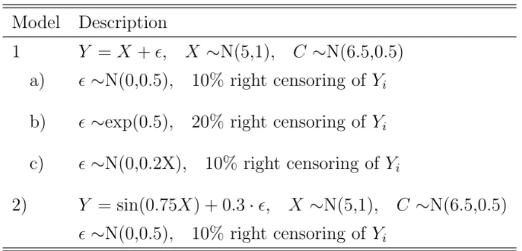
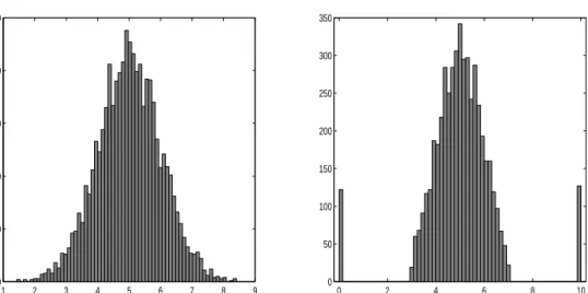
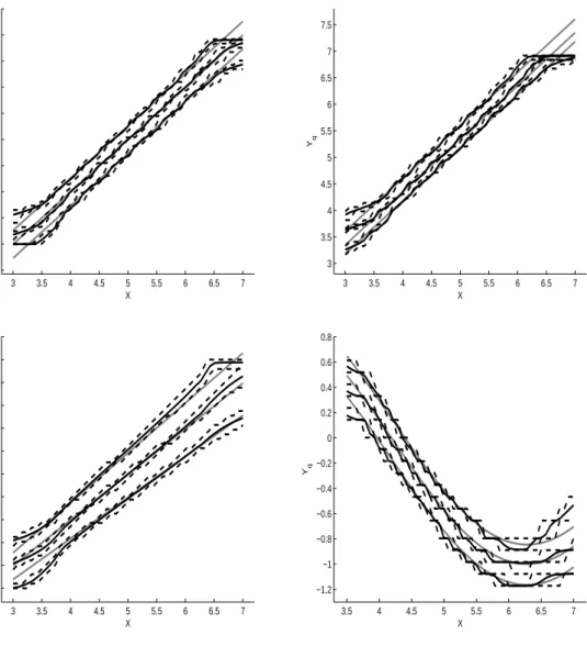
(10) denominator of our estimator then converge to the conditional probabilities P (Y = y|d = 1, X = x) and P (Y ≥ y|X = x), respectively. Akritas (1994) also derives an expression for the covariance function, but it is alternatively possible to use the bootstrap (Akritas, 1992). We follow the second approach because it appears to be more simple.. 3. Simulation. We analyse the behaviour of estimator (4) for different functional relationships between X and Y and different distributions of error terms. We draw k = 500 random samples of size 500 or 5,000 for the models given in table 1. The specification of model 2 is adapted from Fan (1992) who investigates the behavior of kernel estimators in the mean regression model. In the following we focus mainly on the 0.3, 0.5 and 0.7 quantile function. As the kernel function we use the Epanechnikov kernel K(x) = max{0.75(1 − x2 ); 0}. As Y and C are continuous we round the τi ’s to the first decimal point. We use three different bandwidths to analyze the sensitivity of the estimates with respect to the bandwidth choice. The mean runtime for one simulation is about 0.5 seconds for 500 observations and 2.5 seconds for 5,000 observations (AMD64 1.4 GHz, 64 Bit Linux, 64BIT Matlab v7.01) where we have 50 grid points on the support of x and 50 grid points on the support of y. This is evidently fast enough for real world applications. In order to investigate the properties of our estimator in presence of a censored regressor, we censor the distribution of X on both sides. νi = 0 if Xi < 3 and νi = 10 if Xi > 7. Figure 1 illustrates the distribution of X and ν. 5% of the observations are on average affected by this data manipulation. Figure 2 presents the mean 0.3, 0.5 and 0.7 quantile functions as well as the 2.5%- and the 97.5%-quantile of the simulation distribution with bn = 0.1 and the true quantile functions. The estimator generally recovers the true shape of the conditional quantile functions. The bias at both sides of the support of ν is due to two reasons: first, our estimator fits locally a constant. Therefore we have a boundary bias that starts at a distance of the bandwidth apart of the edge of observations. Second, Gn is inconsistent below cl 6.

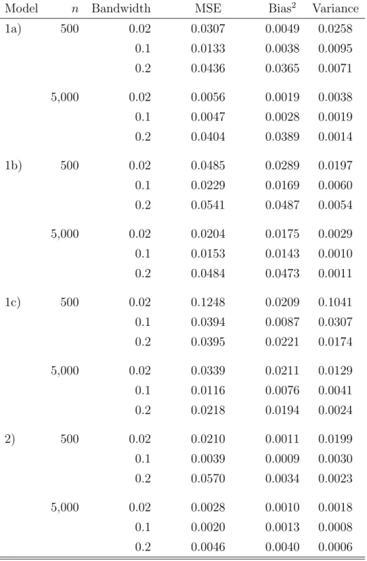
(11) Model. Description. 1. Y = X + ², X ∼N(5,1), C ∼N(6.5,0.5). 2). a). ² ∼N(0,0.5), 10% right censoring of Yi. b). ² ∼exp(0.5), 20% right censoring of Yi. c). ² ∼N(0,0.2X), 10% right censoring of Yi Y = sin(0.75X) + 0.3 · ², X ∼N(5,1), C ∼N(6.5,0.5) ² ∼N(0,0.5), 10% right censoring of Yi Table 1: Models for simulation study.. and above cu . This aggravates the boundary bias but it does not affect interior estimates. Since we use the SNN smoothing we have a variable bandwidth given ν. The low density of ν at the boundaries implies a larger bandwidth given ν than in the interior of the support of ν. Table 2 presents the mean squared error (MSE), the squared bias and variance of the estimator for the different models. We only present the result for the median as the results for other quantiles (α = 0.3 and α = 0.7) do not differ remarkably. The MSE is calculated by using k. M SE =. m. 1 XX (q̂j (Xi ) − q(Xi ))2 . km i=1 j=1. It is apparent from the table that the estimator has the typical behaviour with respect to the bandwidth choice. In particular, there is a bandwidth which minimises the MSE. In our small numerical exercise it takes on the smallest value for bn = 0.1 in all models, but this would certainly not be the case for other simulation designs.. 4. Empirical Results. We estimate conditional quantile functions with a sample of German administrative individual unemployment duration data. It is extracted from the IAB-Employment Sample 1975-2001 (IABS-R01) which contains daily employment trajectories of 7.

(12) Model 1a). 500. 500. 5,000. 2). Variance. 0.02. 0.0307. 0.0049. 0.0258. 0.1. 0.0133. 0.0038. 0.0095. 0.2. 0.0436. 0.0365. 0.0071. 0.02. 0.0056. 0.0019. 0.0038. 0.1. 0.0047. 0.0028. 0.0019. 0.2. 0.0404. 0.0389. 0.0014. 0.02. 0.0485. 0.0289. 0.0197. 0.1. 0.0229. 0.0169. 0.0060. 0.2. 0.0541. 0.0487. 0.0054. 0.02. 0.0204. 0.0175. 0.0029. 0.1. 0.0153. 0.0143. 0.0010. 0.2. 0.0484. 0.0473. 0.0011. 0.02. 0.1248. 0.0209. 0.1041. 0.1. 0.0394. 0.0087. 0.0307. 0.2. 0.0395. 0.0221. 0.0174. 0.02. 0.0339. 0.0211. 0.0129. 0.1. 0.0116. 0.0076. 0.0041. 0.2. 0.0218. 0.0194. 0.0024. 0.02. 0.0210. 0.0011. 0.0199. 0.1. 0.0039. 0.0009. 0.0030. 0.2. 0.0570. 0.0034. 0.0023. 0.02. 0.0028. 0.0010. 0.0018. 0.1. 0.0020. 0.0013. 0.0008. 0.2. 0.0046. 0.0040. 0.0006. 500. 5,000. 1c). Bias2. Bandwidth. 5,000. 1b). MSE. n. 500. 5,000. Table 2: Simulation results for α = 0.5.. 8.

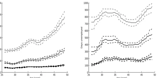
(13) 250. 350. 300 200 250 150. 200. 150. 100. 100 50 50. 0. 1. 2. 3. 4. 5 x. 6. 7. 8. 0. 9. 0. 2. 4. ν. 6. 8. 10. Figure 1: Distribution of X (left) and observed distribution of ν (right). about 1.1 Mio indivduals from West-Germany and about 200K individuals from East-Germany. It is a 2% random sample of the socially insured workforce. See Hamann et al. (2004) for further details on this data. For our estimations we use the same sample of unemployment spells that is also used by Fitzenberger and Wilke (2007). However, we restrict attention to the age, the gender and the last daily wage before unemployment for all ”nonemployment” spells starting in 1996 or 1997 in West-Germany. Our sample comprises 21, 685 observations. We use the estimator defined in (4) to estimate smooth nonparametric conditional quantile functions of the distribution of unemployment duration conditional to age or previous wage level. According to our simulations, the bandwidth should not be too large or too small. After checking that the quality of our results does not change with small variations in the bandwidth, we decided to use bn = 0.1. For the estimation of the standard errors we use the bootstrap method by drawing 500 resamples with replacement and plot the 5%− and the 95%- quantiles of the bootstrap distribution. Figure 3 shows the estimation results conditional to age for the 0.3-, 0.5- and the 0.7-quantile for males (left) and females (right) with the 5- and 95%-bootstrap quantiles for each quantile. While age plays a less important role for the shortly unemployed men and women, there is a strongly positive influence of age in the 9.

(14) 7.5 7.5 7 7 6.5 6.5. 6. 6 Yq. Yq. 5.5 5. 5.5 5. 4.5. 4.5. 4. 4. 3.5. 3.5. 3. 3. 2.5 3. 3.5. 4. 4.5. 5 X. 5.5. 6. 6.5. 7. 3. 8. 0.8. 7.5. 0.6. 7. 0.4. 6.5. 3.5. 4. 4.5. 5 X. 5.5. 6. 6.5. 7. 0.2. 6 0 Yq. Yq. 5.5 5. −0.2 −0.4. 4.5. −0.6. 4 3.5. −0.8. 3. −1. 2.5. −1.2 3. 3.5. 4. 4.5. 5 X. 5.5. 6. 6.5. 7. 3.5. 4. 4.5. 5. 5.5. 6. 6.5. 7. X. Figure 2: Simulation of model 1a (top left), model 1b (top right), model 1c (bottom left) and model 2 (bottom right); mean of the estimates of the quantile functions for (from bottom to top) α=0.3;0.5;0.7, the 2.5%- and the 97.5%-bootstrap quantile for each estimate (dashed lines) and the true model (lighter lines) for 5,000 observations and a kernel bandwidth b = 0.1.. 10.

(15) group of the long-term unemployed men. The pattern for the longer unemployed women isn’t as clear as it is for men, especially not for the 0.7-quantile. According to Lechner (1997) the probability of fertility has its maximum between the age of 26 and 30. This fact could offer a possible explanation for the peak of the curve at the age of 32: At that age, mothers have passed their maternity leave and claim remaining entitlements for unemployment benefits. However, some of them may not actually look for a job. Note that both ends of the estimated curves can have some boundary bias. For the estimations conditional to the previous daily wage we only use the males. This is because of some lack of information about part-time work which is rather frequent for females. The histogram in figure 4 (left) shows the distribution of the variable ”previous wage”. The value ”0” means an income below and the value ”200” means an income above the social security contribution ceiling (”Beitragsbemessungsgrenze”). For this reason we only plot results for the 10% − 90%-quantile of former income. The right panel of Figure 4 shows a weakly decreasing conditional 0.3 quantile function. At the 0.5 and 0.7-quantiles, the decrease is much stronger until a previous wage level of 65 Euro per day. As discussed in detail by Fitzenberger and Wilke (2007), the much longer long-term unemployment periods for low wage individuals are probably related with high and almost time invariant wage replacement rates. The income transfers for this group generally do not decrease after expiration of unemployment benefits as they often do not exceed the level of social benefits. It is unlikely that presented estimates have a boundary bias as we only report them in the range 20-120 EUR. Biewen and Wilke (2005) and Fitzenberger and Wilke (2007) apply the semiparametric hazard rate model, the accelerated failure time model and Box-Cox quantile regression to similar or the same data. While there is no evident contradiction between their and our results, we claim that the estimated conditional quantile functions of this paper give more detailed insights on the conditional distribution of unemployment duration.. 11.

(16) 1200. 1000 900 800 700. 800. Days unemployed. Days unemployed. 1000. 600. 400. 600 500 400 300 200. 200. 100 0 25. 30. 35. 40 Age (years). 45. 0 25. 50. 30. 35. 40. 45. 50. Age (years). Figure 3: Estimated quantile functions conditional on age (for α = 0.3; 0.5; 0.7 from bottom to top); left: males, right: females; dashed lines: 5%- and the 95%bootstrap quantile for each estimate.. 1200. 1000. 1000. 800. 800. Days unemployed. 1200. 600. 400. 200. 0. 600. 400. 200. 0. 50. 100 150 Previous daily wage (in EURO). 0. 200. 20. 40. 60 80 Previous daily wage in EURO. 100. 120. Figure 4: left: Histogram of the previous wage for males; right: Estimated quantile functions conditional on the previous wage (for α = 0.3; 0.5; 0.7 from bottom to top) for males; dashed lines: 5%- and the 95%-bootstrap quantile for each estimate.. 12.

(17) 5. Conclusion and Outlook. This paper suggests simple nonparametric estimators for the conditional hazard rate and the conditional quantile function when the distribution of the response and of the regressor are both censored. Our simulations and our application show that it is a meaningful and fast tool for data exploration that works without strong assumptions. Resulting estimates can be used for the specification of a statistical model of more structure. There are several interesting topics for future research that may be beneficial for applied analysis: one could introduce a partially linear approach or one may establish a link to the approach of Portnoy (2004). One could allow for discrete regressors or an additive nonparametric structure. In our application we found some evidence that the conditional quantile functions possess different shapes across quantiles. Therefore one may also develop a test for shape invariance of those functions. Such a test would then provide elaborate information whether a more structural model, such as censored quantile regression, would require different model specifications across the quantiles. It would also be straightforward to extend the estimator given in (2) to multivariate X of dimension k = 1, . . . , D by applying the idea of product kernels. The estimator for the conditional hazards rates is then µ ¶ Pn Q Gn (xk )−Gn (νik ) i=1 1τi =y 1di =1 kK bnk µ ¶ . hn (y|x) = Pn Q Gn (xk )−Gn (νik ) i=1 1τi ≥y kK bnk Note that this estimation strategy, however, suffers from the curse of dimensionality. For multivariate regressors see also Dabrowska (1995).. References Akritas, M.G. (1992). ”Boostrapping the nearest neighbor estimator of a bivariate function”, unpublished manuscript. Akritas, M.G. (1994). ”Nearest neighbor estimation of a bivariate distribution under random censoring”, Annals of Statistics, 22, 1299–1327. 13.

(18) Beran, R. (1981). ”Nonparametric Regression with Randomly Censored Survival Data”, Technical Report, University of California, Berkeley, CA. Biewen, M. and Wilke, R.A. (2005).. ”Unemployment duration and the length. of entitlement periods for unemployment benefits: do the IAB employment subsample and the German Socio-Economic Panel yield the same results?” Allgemeines Statistisches Archiv , 89(2), 409–425. Dabrowska, D.M. (1995). ”Nonparametric regression with censored covariates”, Journal of Multivariate Analysis, 54(2), 253–283. Fan, J. (1992). ”Design-adaptive Nonparametric Regression”, Journal of the American Statistical Association, Col. 87, No. 420, 998–1004. Fitzenberger, B. and Wilke, R.A. (2006), ”Using Quantile Regression for Duration Analysis”, Allgemeines Statistisches Archiv, 90(1), 103–118. Fitzenberger, B. and Wilke, R.A. (2007), ”New Insights on Unemployment Duration and Post Unemployment Earnings in Germany: Censored Box-Cox Quantile Regression at Work”, ZEW Discussion Paper 07-007. Hamann, S., Krug, G., Köhler, M., Ludwig-Mayerhofer, W. and Hacket, A. (2004). Die IAB-Regionalstichprobe 1975-2001: IABS-R01” ZA-Information 55, S. 36-42 Kaplan, E. L., and P. Meier (1958), ”Nonparametric estimation from incomplete observations”, Journal of the American Statistical Association, 53, 457–481. Koenker, R. and Bilias, Y. (2001), ”Quantile Regression for Duration Data: A Reappraisal of the Pennsylvania Reemployment Bonus Experiments”, Empirical Economics, Vol.26, 199–220. Koenker, R. and Geling, O. (2001), ”Reappraising Medfly Longevity: A Quantile Regression Survival Analysis”, Journal of the American Statistical Association, Vol.96, No.454, 458–468.. 14.

(19) Lechner, M. (1997), ”Eine empirische Analyse der Geburtenentwicklung in den neuen Bundesländern”, Beiträge zur angewandten Wirtschaftsforschung, No. 551-97. Machado, J.A.F. and Portugal, P. (2002), ”Exploring Transition Data through Quantile Regression Methods: An Application to U.S. Unemployment Duration”, in: Statistical data analysis based on the L1-norm and related methods – 4th International Conference on the L1-norm and Related Methods (Ed. Yadolah Dodge), Basel: Birkhäuser. McKeague, I.W. and Utikal K.J. (1990), ”Inference for a Nonlinear Counting Process Regression Model”, Annals of Statistics, 18, 1172–1185. Portnoy, S. (2004), ”Censored Regression Quantiles”, Journal of the American Statistical Association, Vol.98, No.464, 1001–1012. Stone, C.J. (1977), ”Consistent nonparametric regression”, Annals of Statistics, 5, 595–645. Van Keilegom, I. (1998), ”Nonparametric Estimation of the Conditional Distribution in Regression with Censored Data”, Ph.D. Thesis, Limburgs Universitair Centrum, Belgium Van Keilegom, I. and Veraverbeke, N. (2001), ”Hazard Rate Estimation in Nonparametric Regression with Censored Data”, Ann. Inst. Statist. Math., 53, 730–745. Yang, S. (1981), ”Linear functions of concomitants of order statistics with applications to nonparametric estimation of a regression function”, Journal of the American Statistical Association, 76, 658–662.. 15.

(20)

No results found