ISSN 1440-771X
Australia
Department of Econometrics and Business Statistics
http://www.buseco.monash.edu.au/depts/ebs/pubs/wpapers/
September 2011
Working Paper 14/11
Estimation in Partially Linear Single-Index Panel
Data Models with Fixed Effects
Estimation in Partially Linear Single–Index
Panel Data Models with Fixed Effects
By Jia Chen∗†, Jiti Gao† and Degui Li†1
∗University of Queensland and †Monash University
Abstract
In this paper, we consider semiparametric estimation in a partially linear single– index panel data model with fixed effects. Without taking the difference explicitly, we propose using a semiparametric minimum average variance estimation (SMAVE) based on a dummy–variable method to remove the fixed effects and obtain consistent estimators for both the parameters and the unknown link function. As both the cross section size and the time series length tend to infinity, we not only establish an asymptotically normal distribution for the estimators of the parameters in the single index and the linear component of the model, but also obtain an asymptotically normal distribution for the nonparametric local linear estimator of the unknown link function. The asymptotically normal distributions of the proposed estimators are similar to those obtained in the random effects case. In addition, we study several partially linear single–index dynamic panel data models. The methods and results are augmented by simulation studies and illustrated by an application to a cigarette– demand data set in the US from 1963–1992.
JEL subject classifications: C13, C14, C23.
Keywords: Fixed effects, local linear smoothing, panel data, semiparametric
estima-tion, single–index models.
1Corresponding author: Department of Econometrics and Business Statistics, Monash University
1. Introduction
Panel data analysis has become increasingly popular in many fields, such as cli-matology, economics and finance. The double–index models enable researchers to estimate complex models and extract information that may be difficult to obtain by applying purely cross–section or time–series models. There exists rich literature on parametric linear and nonlinear panel data models. For an overview of statistical inference and econometric analysis of parametric panel data models, we refer to the books by Baltagi (1995), Arellano (2003) and Hsiao (2003). As in both the cross section and time series cases, parametric panel data models may be misspecified, and estimators obtained from such misspecified models are often inconsistent. To address such issues, some nonparametric methods have been used in both panel data model estimation and specification testing. Recent studies include Ullah & Roy (1998), Hjellvik et al (2004), Cai & Li (2008), Henderson et al (2008), and Mammen et al
(2009).
In the multivariate setting with more than three covariates, the underlying re-gression function cannot be estimated with reasonable accuracy due to the so–called “curse of dimensionality”. How to circumvent the curse of dimensionality is an im-portant issue in both nonlinear time series and panel data analysis. Many approaches have been developed to address this issue (see, recent books by Fan & Yao 2003, Gao 2007, Li & Racine 2007 for example). One commonly–used approach is the semi-parametric partially linear modeling. An advantage of the semisemi-parametric partially linear modeling is that any existing information concerning possible linearity of some of the components can be taken into account in such models. This has been studied extensively in both the time series and panel data cases (see, for example, Gao 2007, Li & Racine 2007).
As is well known, however, the nonparametric components in the partially linear models may only accommodate covariates X with low dimension and they are also subject to the curse of dimensionality when the dimension ofXis larger than three. To address this issue, we use the dimension reduction technique of single–index modelling. Specifically, we consider a partially linear single–index panel data model of the form
where Zit = (Zit,1,· · · , Zit,d)⊤ and Xit = (Xit,1,· · · , Xit,p)⊤ are the respective d–
dimensional and p–dimensional covariate vectors, β0 = (β0,1,· · ·, β0,d)⊤ and θ0 =
(θ0,1,· · · , θ0,p)⊤ are unknown parameters with dimensions d and p, respectively, η(·)
is an unknown link function, αi are unobserved time-invariant individual effects, and
vit are the random errors. Note thatZit can be either continuous or discrete random
variables, whileXit are assumed to be continuous random variables.
Model (1.1) is called a fixed effects model if {αi} is correlated with {Zit} and
(or) {Xit} with an unknown correlation structure. Model (1.1) is called a random
effects model if{αi}is uncorrelated with both{Zit}and{Xit}. In this paper, we are
concerned with the fixed effects case. For the purpose of identification, we assume that
(i)
n
∑
i=1
αi = 0, (ii) ∥θ0∥= 1 and the first component of θ0 is positive, (1.2)
where∥·∥:=∥·∥2 is the L2–distance. (i) is a commonly used identification condition
on the fixed effects (see, for example, Su & Ullah 2006, Sun et al 2009). (ii) is an identification condition for the single–index structure in our model (see, for example, Carrollet al 1997, Xiaet al 2002).
Model (1.1) covers many interesting panel data models. When β0 ≡ 0, model (1.1) reduces to a single–index panel data model (Bai et al 2009). When Xit are
scalar, model (1.1) becomes to a partially linear panel data model with fixed effects (Su & Ullah 2006). When β0 ≡ 0 and η(·) is known, model (1.1) is a generalized linear panel data model with fixed effects (Hsiao 2003).
Existing literature mainly focuses on both nonparametric and semiparametric es-timation of random effects panel data models (see, for example, Li & Stengos 1996, Ullah & Roy 1998, Henderson & Ullah 2005). Note that the random effects estima-tors are inconsistent if the true model is one with fixed effects. In this paper, we will develop a semiparametric estimation method associated with a local linear dummy variable approach for model (1.1). The estimation method is consistent under either
the random effects setting or the fixed effects setting.
In this paper, we also allow that either Zit or Xit contain time lagged values of
Yit. In this case, model (1.1) covers several partially linear single–index dynamic
geometrically ergodic under some mild conditions, when it is generated by a type of partially linear autoregressive models. This implies that stationarity and mixing conditions on the underlying process are satisfied for each i ≥ 1. Furthermore, we apply the partially linear single–index panel data model to analyze the dynamic de-mand of cigarettes based on a panel data set from 46 states in the US. The data set contains the consumption of cigarettes, the lagged consumption of cigarettes, the average retail price, disposable income and the minimum price of cigarettes in any neighboring state. Baltagi et al (2000) and Mammen et al (2009) respectively used a parametric linear model and a nonparametric additive model to analyze the rela-tionship among the variables. From the study by Mammen et al (2009), we can see that there is some linear relationship between the consumption of cigarettes and its lagged consumption. This suggests that model (1.1) might be a better option for such a data set (see Section 5 for detail).
The main contribution of this paper can be summarized as follows. We first propose using a semiparametric minimum average variance estimation (SMAVE) ap-proach associated with a dummy variable method to estimate the parametersβ0 and
θ0 as well as the unknown link functionη(·). Under certain regularity conditions, we
are able to establish asymptotically normal distributions for the proposed parametric estimators and nonparametric estimator when both n and T tend to infinity. Fur-thermore, we find that the dummy variable approach proposed for the fixed effects case enables us derive the same asymptotically normal distributions as in the case where random effects are involved.
The rest of the paper is organized as follows. In Section 2, we introduce the so–called SMAVE method to estimate β0, θ0 and η(·). Section 3 establishes the
asymptotic theory for the proposed estimators. Section 4 discusses some autoregres-sion extenautoregres-sions of the proposed model. Section 5 illustrates the performance of the proposed models and estimation methods using both simulated and real data exam-ples. Technical assumptions and proofs of the main results are provided in Appendices A–C. An additional appendix as Appendix D is given in a supplemental document.
2. Dummy variable based SMAVE approach
methods have been introduced (see, for example, Carroll et al 1997, Liang et al
2010, Wang et al 2010 for the profile likelihood method; Yu & Ruppert 2002 for the penalized spline method; Xia and H¨ardle 2006 for the SMAVE method). However, these methods cannot be readily used for the panel data model (1.1) due to the presence of the fixed effects. The fixed effects, which are absent in time series models, have to be eliminated in the estimation procedure so that consistent estimators can be constructed. In linear panel data models, the conventional method of removing the fixed effects is differencing, i.e., deducting either a cross–time average or the observations for the previous time period from the observations for the current time period (Henderson et al 2008). However, due to the single–index structure in model (1.1), the differencing will complicate the estimation of the link function. Hence, we will develop an estimation procedure based on a local linear dummy variable approach, which is motivated by the least squares dummy variable approach used for parametric panel data analysis (Hsiao 2003). In the dummy variable approach, the unobserved fixed effects are brought explicitly into the model (1.1) and are treated as the coefficients of the model. Having re-specified model (1.1) in this way, we can estimate it by using the SMAVE method.
Apart from the fixed effects, another factor in the estimation of model (1.1) that is different from the estimation of corresponding time series models is the involvement of two indices: the time index t and the individual index i, which, as one might expect, will add further complexity to the estimation of model (1.1). We will establish asymptotic theory for the proposed estimators, as both the time–series dimension T and the cross–sectional dimensionntend to infinity, by using the joint limit approach introduced by Phillips and Moon (1999). The detailed proofs for such joint limiting distribution results are more complicated than those for the asymptotic distribution theory of time series models.
We next introduce the SMAVE method, which estimates both the parameters and the unknown link function by minimizing a single common loss function. The SMAVE method was first introduced by Xia et al (2002) for single–index time series models, Recently, Xia (2006) established an asymptotic theory for this approach in time series models and Xia & H¨ardle (2006) extended the approach and its asymptotic theory to partially linear single–index time series models. However, extending this approach to
the partially linear single–index panel data model (1.1) is challenging for the reasons stated above. To address these issues, we will combine the dummy variable approach with the SMAVE method and construct root–nT consistent parametric estimators.
We first introduce some notations for brevity of the presentation of our estimation method. Let Y= (Y11,· · · , Y1T, Y21,· · · , YnT)⊤, Z= (Z11,· · · ,Z1T,Z21,· · · ,ZnT)⊤, V= (v11,· · · , v1T, v21,· · ·, vnT)⊤, η(X,θ) =(η(X⊤11θ),· · ·, η(X⊤1Tθ), η(X⊤21θ),· · · , η(X⊤nTθ))⊤, D0 =In⊗eT, α0 = (α1,· · ·, αn)⊤,
whereIn is then×n identity matrix, eT is a T–dimensional vector with all elements
being 1, and⊗denotes the Kronecker product. With these notations, we can rewrite model (1.1) as
Y=Zβ0+η(X,θ0) +D0α0+V. (2.1)
Furthermore, by the identification assumption
n ∑ i=1 αi = 0, we have α1 = − n ∑ i=2 αi.
LettingD= [−en−1, In−1]⊤⊗eT and α= (α2,· · · , αn)⊤, (2.1) can then be rewritten
as
Y=Zβ0+η(X,θ0) +Dα+V. (2.2)
For Xit close to x∈Rp, we have the following local linear approximation:
η(X⊤itθ0)≈η(x⊤θ0) +η′(x⊤θ0)(Xit−x)⊤θ0,
where η′(u) is the derivative of η(u) at u. The basic idea of the SMAVE method is to minimize n ∑ i=1 T ∑ t=1 [ Y−Zβ−Dα−(enT,Xit(θ)) (ait, bit)⊤ ]⊤ Wit [ Y−Zβ−Dα−(enT,Xit(θ)) (ait, bit)⊤ ] (2.3) with respect toβ,θ, and (ait, bit)⊤, where
Xit(θ) =
(
(X11−Xit)⊤θ,· · ·,(X1T −Xit)⊤θ,(X21−Xit)⊤θ,· · · ,(XnT −Xit)⊤θ
)⊤
and Wit = diag(w11,it,· · · , w1T,it, w21,it,· · ·, wnT,it) is a diagonal matrix with its elements satisfying n ∑ j=1 T ∑ s=1
To solve the minimization problem (2.3), we will use an iterative procedure, which is detailed as follows.
Step (i): For given β and θ, minimizing
[ Y−Zβ−Dα−(enT,Xit(θ)) (ait, bit)⊤ ]⊤ Wit [ Y−Zβ−Dα−(enT,Xit(θ)) (ait, bit)⊤ ] (2.4) with respect toα, we get
αit = ( D⊤WitD )−1 D⊤Wit [ Y−Zβ−(enT,Xit(θ)) (ait, bit)⊤ ] . (2.5)
Then, lettingα in (2.4) replaced by the right hand side of (2.5) and minimizing the resulting weighted least squares with respect to (ait, bit)⊤, we obtain the local linear estimator of(η(X⊤itθ), η′(X⊤itθ))⊤:
(ait, bit)⊤=
(
X⊤it,∗(θ)WitXit,∗(θ)
)−1
X⊤it,∗(θ)Wit(Yit,∗−Zit,∗β), (2.6) where Xit,∗(θ) = [ InT −D ( D⊤WitD )−1 D⊤Wit ] (enT,Xit(θ)), Yit,∗=Y−D ( D⊤WitD )−1 D⊤WitY, Zit,∗=Z−D ( D⊤WitD )−1 D⊤WitZ.
Step (ii): For each pair (i, t), substituteαand (ait, bit)⊤in (2.3) with the right hand sides of (2.5) and (2.6) and solve the resulting minimization problem with respect toβand θ to obtain (β⊤,θ⊤)⊤ = Z ⊤ ∗WZ∗ Z⊤∗WX∗ X⊤ ∗WZ∗ X⊤∗WX∗ −1 Z ⊤ ∗ X⊤ ∗ W(Y∗−A∗), (2.7) where W= diag (W11,· · · ,W1T,W21,· · ·,WnT), Y∗ = ( Y11⊤,∗,· · · , Y1⊤T,∗, Y21⊤,∗,· · · , YnT ,⊤ ∗ )⊤ , Z∗ = ( Z⊤11,∗,· · ·,Z⊤1T,∗,Z⊤21,∗,· · ·,Z⊤nT,∗ )⊤ , X∗ = ( b11X⊤11,∗,· · · , b1TX⊤1T,∗, b21X⊤21,∗,· · · , bnTX⊤nT,∗ )⊤ , Xit,∗= [ InT −D ( D⊤WitD )−1 D⊤Wit ] Xit,
Xit = ((X11−Xit),· · ·,(X1T −Xit),(X21−Xit),· · ·,(XnT −Xit))⊤,
A∗ = ( a11e⊤11,∗,· · · , a1Te⊤1T,∗, a21e⊤21,∗,· · ·, anTe⊤nT,∗ )⊤ , eit,∗= [ InT −D ( D⊤WitD )−1 D⊤Wit ] enT.
Step (iii): With the updated values of βand θ, repeat the above two steps until conver-gence.
As in Xiaet al(2002), we use two sets of weights in the above iterative procedure. The first is a set of multidimensional kernel weights defined as
wjs,it = H((Xjs−Xit)/h1) n ∑ j=1 T ∑ s=1 H((Xjs−Xit)/h1) , (2.8)
whereH(·) is ap–variate symmetric kernel function and h1 is a bandwidth. Choosing any
d–dimensional vector β and p–dimensional vectorθ with∥θ∥= 1 and following the above iterations, we can obtain initial estimators of β0 and θ0, which will later be shown to be
consistent. The initial estimators ofβ0 andθ0 are denotedβe and eθ, respectively. However,
the estimators based on the p–variate kernel H(·) are not efficient due to the “curse of dimensionality”. To improve the efficiency, we then use a set of single–index weights which are defined as wθjs,it= K ( (Xjs−Xit)⊤θ/h2 ) n ∑ j=1 T ∑ s=1 K((Xjs−Xit)⊤θ/h2) , (2.9)
where K(·) is a univariate symmetric kernel function and h2 is a bandwidth. Using the
initial estimatesβe andeθand following steps (i)–(iii) with the single–index weights, we then obtain the final estimatorsβb and bθ. By substitutingβ,θ and X⊤itθ in (2.6) withβb,θband
u, we obtain the estimator of η(u), which is denoted bη(u).
3. Asymptotic theory
In this section, we establish the weak consistency ofβe and eθ and then give the asymp-totically normal distributions of βb, bθ and the nonparametric local linear estimate of the link function.
Theorem 3.1. Let Assumptions A1–A7 listed in Appendix A hold. Then, we have
e
β−β0=oP(1) and θe−θ0=oP(1). (3.1) The proof of Theorem 3.1 is given in Appendix B below. Theorem 3.1 establishes the weak consistency of βe and eθ. Note that the detailed proof of Theorem 3.1 and related technical lemmas in Appendix D of the supplemental document indicate that one can pos-sibly strengthen the weak consistency result to strong consistency. The consistency of the initial estimators ofβ0 andθ0 will help us to establish the root-nT convergence of the final
Before giving the asymptotic distribution for βb and bθ, we introduce some notations. Let Zeit,θ =Zit−vθ(Xit) and Xeit,θ =Xit−µθ(Xit), wherevθ(x) =E
( Z11|X⊤11θ =x⊤θ ) and µθ(x) =E(X11|X⊤11θ=x⊤θ ) . Define Σ0 = Σ0(1) Σ0(2) Σ⊤0(2) Σ0(3) and Σ1 = Σ1(1) Σ1(2) Σ⊤1(2) Σ1(3) , (3.2) where Σ0(1) =E ( e Z11Ze⊤11 ) , Σ0(2) =E [ e Z11η′(X⊤11θ0)Xe⊤11 ] , Σ0(3) =E [( η′(X⊤11θ0) )2 e X11Xe⊤11 ] , Σ1(1) = ∞ ∑ t=−∞ E ( e Zi1Ze⊤itvi1vit ) , Σ1(2) = ∞ ∑ t=−∞ E [ e Zi1η′(X⊤itθ0)Xe⊤itvi1vit ] and Σ1(3) = ∞ ∑ t=−∞ E [ η′(X⊤i1θ0)η′(X⊤itθ0)Xei1Xe⊤itvi1vit ] .
The asymptotically normal distribution ofβb and bθ is given in the following theorem.
Theorem 3.2. Let AssumptionsA1–A7andB1–B4 listed in Appendix A hold. Then, as
n, T → ∞ simultaneously, we have √ nT βb−β0 b θ−θ0 −→d N(0, Σ0−1Σ1Σ−01 ) , (3.3)
where 0 is a null–vector of dimension d+p.
Theorem 3.2 shows that the final estimators resulting from the iterative procedure as-sociated with the second set of weights achieve the root–nT rate of convergence. The asymptotic distribution in (3.3) can be regarded as a natural and substantial extension of existing results for time series case, such as Theorems 2 and 3 in Carroll et al (1997), Theorem 1 in Xia & H¨ardle (2006) and Theorem 1 in Liang et al (2010). Furthermore, if we assume that the error process {vit} is independent of {Zit} and {Xit}, and vit are independent and identically distributed (i.i.d.) over i and t, the asymptotic variance in (3.3) can be reduced to σ2Σ−01, where σ2 =E[v2it]. This implies that the SMAVE method achieves an semiparametrically efficient bound (see Carroll et al 1997 for details).
Under some mild conditions, we can show that the joint limit as both n and T tend to infinity is identical to the sequential limit as T → ∞ first and then n → ∞ or the
sequential limit asn→ ∞first and thenT → ∞(see, for example, Phillips & Moon 1999). Additionally, we also find that, asT → ∞, the dummy variable approach proposed for the fixed effects case provides the same asymptotically normal distribution as in the case where random effects are involved. To the best of our knowledge, this is a set of new findings for this type of nonlinear panel data models.
Let us turn to the asymptotic distribution of the the nonparametric estimator of the link function. Letµk=∫ ukK(u)du,νk =
∫
ukK2(u)du, bη(u) = 12µ2η′′(u)h22 and σ2η(u) =
ν0σ2θ0(u)fθ−01(u), where σ2θ0(u) = E(vit2|X⊤itθ0 = u) and fθ0(·) is the density function of
X⊤itθ0.
Theorem 3.3.Let the conditions of Theorem 3.2 hold. As n, T → ∞ simultaneously,
√ nT h2 ( b η(x⊤bθ)−η(x⊤θ0)−bη(x⊤θ0) ) d −→N ( 0, σ2η(x⊤θ0) ) . (3.4)
From the above theorem, the forms of the bias term bη(·) and the asymptotic variance term σ2η(·) are similar to those of the local linear estimator for panel data models with random effects (see, for example, Theorem 3 in Cai & Li 2008). This implies that the dummy variable approach proposed for the fixed effects case has similar asymptotically normal distribution to that in the random effects case.
The proofs of Theorems 3.2 and 3.3 are given in Appendix C.
4. Dynamic partially linear single–index panel data models
This section introduces several dynamic models where the regressorsZitand (or) Xitin (1.1) contain time–lagged values ofYit. Three types of partially linear single–index dynamic panel data models are considered.
Case (i) LettingZit= (Yi,t−1,· · ·, Yi,t−d)⊤, model (1.1) then becomes
Yit= d
∑
j=1
Yi,t−jβ0,j+η(X⊤itθ0) +αi+vit, 1≤i≤n,1≤t≤T. (4.1) For each i, suppose that {Xit : t ≥ 1} and {vit : t ≥ 1} are two i.i.d. sequences, and (Xit, vit) are independent of Yi,t−j,j ≥1. Then, a sufficient condition for the geometrical ergodicity of{Yit: t≥1}for each iis that
yd−β0,1yd−1− · · · −β0,d−1y−β0,d̸= 0 for any |y| ≥1, (4.2) which also leads to the stationarity of {Yit: t≥1}.
Case (ii) Consider the case where Xit contain time–lagged values of Yit with Xit = (Yi,t−1,· · · , Yi,t−p)⊤. Model (1.1) then becomes
Yit=Z⊤itβ0+η ∑p j=1 Yi,t−jθ0,j +αi+vit, 1≤i≤n,1≤t≤T. (4.3) For each i, suppose that {Zit : t ≥ 1} and {vit : t ≥ 1} are two i.i.d. sequences, and (Zit, vit) are independent of Yi,t−j,j≥1. Furthermore, assume that for anyu∈R,
|η(u)| ≤λ∗|u|/√p+c∗, (4.4) where 0< λ∗ <1 and 0< c∗ <∞. Then, following the same argument as in Example 3.5 of An and Huang (1996), we can show that{Yit: t≥1}is geometrically ergodic for eachi.
Case (iii) Consider the case where bothZit andXit contain time–lagged values ofYit. In this case, (1.1) becomes
Yit= d ∑ j=1 Yi,t−jβ0,j+η ∑p j=1 Yi,t−jθ0,j +αi+vit, 1≤i≤n,1≤t≤T. (4.5) Xiaet al(1999) considered the time series case of (4.5) withαi≡0 and gave some conditions for the model to be identifiable. We now consider the geometrical ergodicity of{Yit: t≥1} in the panel data model (4.5) withαi ̸= 0 generally. Letηi(u) =η(u) +αi. Then (4.5) can be rewritten as Yit= d ∑ j=1 Yi,t−jβ0,j+ηi ∑p j=1 Yi,t−jθ0,j +vit. (4.6)
Suppose that β0,1, · · ·, β0,d satisfy (4.2), max
i |αi| < ∞, |ulim|→∞ ηi(u) u = |ulim|→∞ η(u) u = 0, and the probability density function of{vit} is positive everywhere. Then it can be shown, following the proof of Theroem 3 in Xia et al (1999), that {Yit : t ≥ 1} is geometrically ergodic for each i.
5. Numerical Examples
In this section, we first carry out a Monte Carlo simulation study to examine the finite sample performance of the proposed estimation method, and then use the proposed model and method to analyze a set of US cigarette demand data.
As introduced in Section 2, we use two sets of weights: one set of multivariate weights for producing consistent initial estimates of β0 and θ0 and a set of single–index weights
p
∏
j=1
K(xj) for the multivariate weights, whereK(u) = 34(1−u2)I(|u| ≤1). Equal bandwidth of h1 = bσX(nT)−1/(4+p) is used for each variate of the multivariate weights, where σbX is the sample standard deviation ofXit, 1≤i≤ n, 1 ≤t≤T. The bandwidthh1 is simply
chosen under the following considerations: firstly it can reduce the computational burden that we suffer from the iterations and secondly the bandwidth choice for the production of initial estimates has little effect on the performance of the final estimates.
For the single–index weights, we use the quadratic kernel K(u) = 34(1−u2)I(|u| ≤
1) and apply a leave–one–unit–out cross validation method for choosing the bandwidth. The leave–one–out cross validation method was proposed in Sun et al (2009) and is an extension of the conventional leave–one–out cross validation method. The idea is to remove
{(Zit,Xit, Yit) : 1≤t≤T} from the data and use the rest of the (n−1)T observations as the training data to obtain estimates ofβ0,θ0 and η(·), which are denoted as βb(−i),θb(−i)
and bη(−i)(·). We thus choose an optimal bandwidth that minimizes a weighted squared prediction error of the form
( Y−B(Z,βb(−))−η(X,bθ(−)) )⊤ M⊤M ( Y−B(Z,βb(−))−η(X,bθ(−)) ) , (5.1) whereM =In×T −T1In⊗(eTe⊤T), B(Z,βb(−)) = ( Z⊤11βb(−1),· · ·,Z⊤1Tβb(−1),Z⊤21βb(−2),· · · ,Z⊤2Tβb(−2),· · ·,Z⊤n1βb(−n),· · ·Z⊤nTβb(−n) )⊤ and η(X,bθ(−)) = ( η(−1) ( X⊤11θ(b−1) ) ,· · ·, η(−1) ( X⊤1Tbθ(−1) ) , η(−2) ( X⊤21bθ(−2) ) ,· · ·, η(−n) ( X⊤nTbθ(−n) ))⊤ .
The weight matrix M is constructed to satisfy M D =0 so that the fixed effect term
Dα is eliminated from (5.1). In fact, M removes a cross-time average from each variable. For example, MY= (Y11−Y1A,· · ·, Y1T −Y1A,· · ·,· · · , Yn1−YnA,· · · , YnT −YnA)⊤, whereYiA= T1 T ∑ t=1 Yit fori= 1,· · ·, n. 5.1. Simulated Examples
Example 5.1. We first use the following data generating process
Yit= 0.3Zit+ sin
{
π
[
(Xit,1+Xit,2+Xit,3)/
√ 3−A ] /(B−A) } +αi+vit, (5.2)
where Zit = 0 for odd t and Zit = 1 for even t, Xit = (Xit,1, Xit,2, Xit,3)⊤ are three–
dimensional random vectors with independent uniform U(0,1) components and are i.i.d. over both i and t, A = 0.3912 and B = 1.3409, αi = 0.5ZiA∗ +ui for i = 1, · · ·, n−1, and αn=− n∑−1 i=1 αi, in whichZiA∗ = 21T T ∑ t=1
(Zit,1+Zit,2) and ui are i.i.d. N(0,0.12) random errors, vit are i.i.d. (over both i and t) N(0,0.12) random variables. In addition, {Zit},
{Xit},{ui}and {vit} are mutually independent.
The true parameters of model (5.2) are β0 = 0.3 andθ0 = (1,1,1)⊤/
√
3, and the link function is η(u) = sin{π(u−A)/(B−A)}. The time series counterpart of this example was used by Carrollet al (1997), Xia and H¨ardle (2006) and Lianget al (2010).
We start the iterative estimation procedure described in Section 2 withθ= (0,1,2)⊤/√5 as the initial values ofθ0. The resulting estimates of the parameters over 200 realizations,
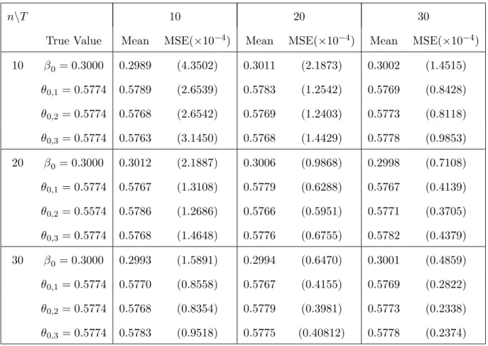
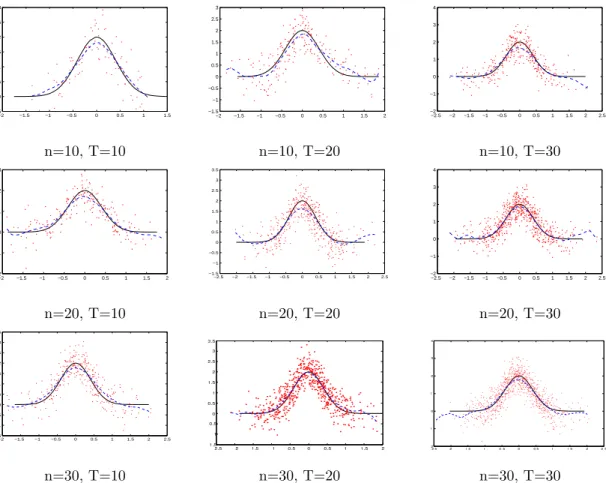
as well as their corresponding mean squared errors (MSEs) for samples of sizes n, T = 10, 20, 30 are summarized in Table 5.1 with the MSEs parenthesized. The estimates of the link functionη(·) from typical realizations of sample sizesn, T = 10, 20, 30 are given in Figure 5.1.
Table 5.1 indicates that the SMAVE method produces accurate estimates of both β0
and θ0, and as either n or T increases, the MSEs of the estimates become smaller and
smaller. Comparison of the results in Table 5.1 with those in the second panel of Table 1 in Xia and H¨ardle (2006) also suggests that the estimates and MSEs here are comparable with those in Xia and H¨ardle (2006).
Example 5.2. Consider the following model
Yit= (2Zit,1+Zit,2)/
√
5 + 2 exp{−(2Xit+Xi,t−1+ 2Xi,t−2)2/3
}
+αi+vit, (5.3)
where Zit = (Zit,1, Zit,2)⊤ are two–dimensional i.i.d. (over both i and t) random vectors
with independent components that have binary distribution withP(Zit,j= 0) =P(Zit,j = 1) = 0.5, j = 1,2, Xit = (Xit, Xi,t−1, Xi,t−2)⊤ in which Xit = 0.4Xi,t−1+xit and xit are i.i.d. (over i and t) and uniformly distributed with xit ∼ U(−1,1), vit are i.i.d. (over i and t) with normal distribution N(0,0.52), αi = 0.5ZiA∗ +ui for i = 1, · · ·, n−1, and
αn=− n∑−1 i=1 αi, in whichZiA∗ = 21T T ∑ t=1
(Zit,1+Zit,2) andui i.i.d.
∼ N(0,0.22). {Zit},{xit},{ui} and {vit} are mutually independent.
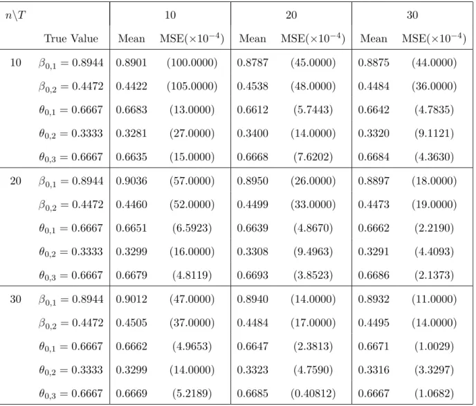
The true parameters of model (5.4) are β0 = (2,1)⊤/√5 andθ0= (2,1,2)⊤/3, and the
true link function isη(u) = 2 exp{−3u2}.
The means as well as the MSEs of the estimates of the parameters over 200 replications are given in Table 5.2. These results indicate that the SMAVE method estimates the
parameters accurately, and its performance (in terms of MSE) improves asnorT increases.
Table 5.1. Means and MSEs of the estimates of the parameters in Example 5.1
n\T 10 20 30
True Value Mean MSE(×10−4) Mean MSE(×10−4) Mean MSE(×10−4) 10 β0= 0.3000 0.2989 (4.3502) 0.3011 (2.1873) 0.3002 (1.4515) θ0,1= 0.5774 0.5789 (2.6539) 0.5783 (1.2542) 0.5769 (0.8428) θ0,2= 0.5774 0.5768 (2.6542) 0.5769 (1.2403) 0.5773 (0.8118) θ0,3= 0.5774 0.5763 (3.1450) 0.5768 (1.4429) 0.5778 (0.9853) 20 β0= 0.3000 0.3012 (2.1887) 0.3006 (0.9868) 0.2998 (0.7108) θ0,1= 0.5774 0.5767 (1.3108) 0.5779 (0.6288) 0.5767 (0.4139) θ0,2= 0.5574 0.5786 (1.2686) 0.5766 (0.5951) 0.5771 (0.3705) θ0,3= 0.5774 0.5768 (1.4648) 0.5776 (0.6755) 0.5782 (0.4379) 30 β0= 0.3000 0.2993 (1.5891) 0.2994 (0.6470) 0.3001 (0.4859) θ0,1= 0.5774 0.5770 (0.8558) 0.5767 (0.4155) 0.5769 (0.2822) θ0,2= 0.5774 0.5768 (0.8354) 0.5779 (0.3981) 0.5773 (0.2338) θ0,3= 0.5774 0.5783 (0.9518) 0.5775 (0.40812) 0.5778 (0.2374)
Table 5.2. Means and MSEs of the estimates of the parameters in Example 5.2
n\T 10 20 30
True Value Mean MSE(×10−4) Mean MSE(×10−4) Mean MSE(×10−4) 10 β0,1= 0.8944 0.8901 (100.0000) 0.8787 (45.0000) 0.8875 (44.0000) β0,2= 0.4472 0.4422 (105.0000) 0.4538 (48.0000) 0.4484 (36.0000) θ0,1= 0.6667 0.6683 (13.0000) 0.6612 (5.7443) 0.6642 (4.7835) θ0,2= 0.3333 0.3281 (27.0000) 0.3400 (14.0000) 0.3320 (9.1121) θ0,3= 0.6667 0.6635 (15.0000) 0.6668 (7.6202) 0.6684 (4.3630) 20 β0,1= 0.8944 0.9036 (57.0000) 0.8950 (26.0000) 0.8897 (18.0000) β0,2= 0.4472 0.4460 (52.0000) 0.4499 (33.0000) 0.4473 (19.0000) θ0,1= 0.6667 0.6651 (6.5923) 0.6639 (4.8670) 0.6662 (2.2190) θ0,2= 0.3333 0.3299 (16.0000) 0.3308 (9.4963) 0.3291 (4.4093) θ0,3= 0.6667 0.6679 (4.8119) 0.6693 (3.8523) 0.6686 (2.1373) 30 β0,1= 0.8944 0.9012 (47.0000) 0.8940 (14.0000) 0.8932 (11.0000) β0,2= 0.4472 0.4505 (37.0000) 0.4484 (17.0000) 0.4495 (14.0000) θ0,1= 0.6667 0.6662 (4.9653) 0.6647 (2.3813) 0.6671 (1.0029) θ0,2= 0.3333 0.3299 (14.0000) 0.3323 (4.7590) 0.3316 (3.3297) θ0,3= 0.6667 0.6669 (5.2189) 0.6685 (0.40812) 0.6667 (1.0682)
5.2. A Real Data Example
The real data example is about the cigarette demand in 46 states of the USA over the period 1963–1992. The data set is from Baltagi et al (2000), who used a linear dynamic panel data model of the form
lnCit =β0+β1lnCi,t−1+θ1lnDIit+θ2lnPit+θ3lnP Nit+uit (5.4)
to analyze the demand for cigarettes, where i= 1, · · ·, 46, denotes the i–th state, t= 1,
· · ·, 29 denotes the t–th year, Cit is the real per capita sales of cigarettes (measured in packs), DTit is the real per capita disposable income, Pit is the average retail price of a
0.2 0.4 0.6 0.8 1 1.2 1.4 1.6 −1 −0.5 0 0.5 1 1.5 0 0.5 1 1.5 −1 −0.5 0 0.5 1 1.5 0 0.2 0.4 0.6 0.8 1 1.2 1.4 1.6 −1.5 −1 −0.5 0 0.5 1 1.5 n=10, T=10 n=10, T=20 n=10, T=30 0 0.2 0.4 0.6 0.8 1 1.2 1.4 1.6 −1 −0.5 0 0.5 1 1.5 0 0.2 0.4 0.6 0.8 1 1.2 1.4 1.6 −1 −0.5 0 0.5 1 1.5 0 0.2 0.4 0.6 0.8 1 1.2 1.4 1.6 1.8 −1.5 −1 −0.5 0 0.5 1 1.5 n=20, T=10 n=20, T=20 n=20, T=30 0 0.2 0.4 0.6 0.8 1 1.2 1.4 1.6 −1 −0.5 0 0.5 1 1.5 0 0.5 1 1.5 2 −1 −0.5 0 0.5 1 1.5 0 0.2 0.4 0.6 0.8 1 1.2 1.4 1.6 1.8 −1 −0.5 0 0.5 1 1.5 n=30, T=10 n=30, T=20 n=30, T=30
Figure 5.1. Curve estimates from single replications of the simulation study of Example 5.1. The solid curves are the true functions η(X⊤itθ0), the dashed curves are the corresponding estimated
functionsbη(X⊤itbθ), the dots denoteYit−Z⊤itβb−αib plotted againstX⊤itbθ.
pack of cigarettes measured in real terms, P Nit is the minimum real price of cigarettes in any neighboring state, and the disturbance termuit in (5.4) is specified as
uit=µi+λt+vit, (5.5)
whereµi denotes a state-specific effect, and λt denotes a year-specific effect, which can also be interpreted as a trend int.
Due to the presence of the time–specific effect or trend λt in all the variables, we first remove the trend from the log-transformed observations as in Mammenet al (2009),
Yit= lnCit−sC(t), V1it =Yi,t−1, V2it= lnDIit−sDI(t),
V3it= lnPit−sP(t), V4it = lnP Nit−sP N(t),
where sC(t), sDI(t), sP(t), and sP N(t) are the nonparametric estimates of the trends in lnCit, lnDIit, lnPit and lnP Nit, i= 1 · · ·, 46, t= 1, · · ·, 29. In Figure 5.3, we give the
−2 −1.5 −1 −0.5 0 0.5 1 1.5 −0.5 0 0.5 1 1.5 2 2.5 3 −2 −1.5 −1 −0.5 0 0.5 1 1.5 2 −1.5 −1 −0.5 0 0.5 1 1.5 2 2.5 3 −2.5 −2 −1.5 −1 −0.5 0 0.5 1 1.5 2 2.5 −2 −1 0 1 2 3 4 n=10, T=10 n=10, T=20 n=10, T=30 −2 −1.5 −1 −0.5 0 0.5 1 1.5 2 −2 −1 0 1 2 3 −2.5 −2 −1.5 −1 −0.5 0 0.5 1 1.5 2 2.5 −1.5 −1 −0.5 0 0.5 1 1.5 2 2.5 3 3.5 −2.5 −2 −1.5 −1 −0.5 0 0.5 1 1.5 2 2.5 −2 −1 0 1 2 3 4 n=20, T=10 n=20, T=20 n=20, T=30 −2 −1.5 −1 −0.5 0 0.5 1 1.5 2 2.5 −1.5 −1 −0.5 0 0.5 1 1.5 2 2.5 3 3.5 n=30, T=10 n=30, T=20 n=30, T=30
Figure 5.2. Curve estimates from single replications of the simulation study of Example 5.2. The solid curves are the true functions η(X⊤itθ0), the dashed curves are the corresponding estimated
functionsbη(X⊤itbθ), the dots denoteYit−Z⊤itβb−αbi plotted againstX⊤itbθ.
scatter plots ofY against V1,V2, V3, andV4. It is clear from Figure 5.3 thatY exhibits strong linearity with V1 (i.e. the lagged variable of Y). For the other three covariates, their linearities with Y are not as strong as that for the lagged-variable. Hence, we define
Zit = V1it and Xit = (V2it, V3it, V4it)⊤, and put Zit in the linear term and Xit in the single-index term of the following model
Yit=Zitβ+g(X⊤itθ) +αi+vit, (5.6)
whereθ = (θ1, θ2, θ3)⊤,αiis a state–specific effect which may include religion, race, tourism, tax, and education. αicorresponds toµiin model (5.4)–(5.5). Furthermore, as we detrended lnCit, lnDIit, lnPit and lnP Nit, the year-specific term λt that appeared in model (5.4)– (5.5) is eliminated from model (5.6).
After applying the estimation method proposed in Section 2 to the data on Yit, Zit,
−0.8 −0.6 −0.4 −0.2 0 0.2 0.4 0.6 0.8 1 −1 0 1 V1 Y −0.8 −0.6 −0.4 −0.2 0 0.2 0.4 0.6 −1 0 1 V2 Y −0.4 −0.3 −0.2 −0.1 0 0.1 0.2 0.3 0.4 0.5 −1 0 1 V3 Y −0.3 −0.2 −0.1 0 0.1 0.2 0.3 0.4 −1 0 1 V4 Y
Figure 5.3. From top to bottom: the scatter plots ofY againstV1,V2,V3, andV4.
−0.25 −0.2 −0.15 −0.1 −0.05 0 0.05 0.1 0.15 0.2 0.25 −0.2 −0.1 0 0.1 0.2 0.3 0.4 0.5
Figure 5.4. Estimated link function and its 95% confidence band. Dots denote Yit−Zitbβ−αib
plotted againstX⊤itbθ. The solid line denotes the estimated link functionbη(X⊤itbθ). The dash-dotted lines represent the 95% confidence band.
5.3. The estimated curve of the link function as well as its 95% confidence band is given in Figure 5.4.
Table 5.3. Estimates of the parameters in the cigarette data example
parameter β θ1 θ2 θ3
estimate 0.8480 0.2594 -0.8735 0.4119
(SD) (0.0073) (0.0217) (0.0099) (0.0260)
Comparison of the results in Table 5.3 with that in Baltagi et al (2000) indicates that our estimate of β is smaller than the estimates of the corresponding coefficient in Baltagi et al(2000), where a value of 0.90 from the OLS method and a value of 0.91 from the GLS method were obtained. In addition, compared withbθ= (0.2112,−0.9404,0.2665)⊤from the OLS andbθ= (0.1602,−0.9503,0.2669)⊤ from the GLS in Baltagiet al(2000), the absolute value of our estimate of θ2 is smaller, while those of θ1 and θ3 are larger (note that due
to the identification condition ∥θ∥ = 1, one has to normalize the estimates of θ in (5.4) before making comparisons). The computed coefficient of determination for model (5.6) is
R2 = 0.9698, which indicates a good fit to the data.
6. Conclusions and Discussion
This paper has considered a partially linear single–index panel data model with fixed effects. A semiparametric minimum average variance estimation method associated with a dummy–variable approach has been proposed to deal with the estimation of both the parametric and nonparametric components of the model. We have shown that the proposed estimators all have asymptotically normal distribution regardless of whether the effects involved are random or fixed. We have then assessed the finite–sample performance of the proposed estimation method through using both simulated and real data examples.
The paper certainly has some limitations. One question is whether the established theory may be extended to the case where both {Xit} amd {Zit} are nonstationary over
t and cross–sectional dependent over i. How to answer such a question should be left in future research.
7. Acknowledgments
The authors would like to thank Xiaohong Chen, Qi Li, Oliver Linton, Liangjun Su and the seminar participants at Monash University, University of Adelaide, University of Queensland, SETA 2011 Conference in Melbourne, and ESAM 2011 Conference in Adelaide.
This project was financially supported by the Australian Research Council Discovery Grants Program under Grant Number: DP0879088.
Appendix A: Assumptions
LetZi = (Zit: 1≤t≤T),Xi = (Xit: 1≤t≤T) andVi= (vit: 1≤t≤T). To derive the consistency of the initial estimates βe and eθ, we need the following set of regularity conditions.
A1(Zi,Xi, Vi),i= 1,· · ·, n, are i.i.d. and{(Zit,Xit, vit) :t≥1}is a stationaryα–mixing sequence with mixing coefficientαi(t) for eachi. Furthermore, there exists a positive coefficient functionα(t) such that
sup i
αi(t)≤α(t) with α(t)≤Cαt−γ0, whereCα>0 andγ0 >
(2+δ∗)(2+δ)
2(δ−δ∗) , in whichδandδ∗are positive constants satisfying
δ > δ∗.
A2The kernel functionH(·): Rd →R+ is a bounded and Lipschitz continuous probabil-ity densprobabil-ity function with a compact support. Furthermore, H(x) is symmetric and
∫
xx⊤H(x)dxis positive definite.
A3The density functionfX(·) of Xit is second–order continuous and has gradient fX′ (·).
Moreover, fX(·) is positive and bounded in X :=
{
x:∥x∥ ≤C(nT)2+1δ }
for any
C >0 and E∥Xit∥2+δ <∞, where ∥ · ∥is the L2–distance and δ was defined in A1.
A4 Let g1(x) := E[Zit|Xit=x] and g2(x) := E
[
ZitZ⊤it|Xit=x
]
. Both g1(x) and g2(x)
have bounded and continuous derivatives. In addition,E∥Zit∥2+δ<∞and
E {
(Zit−E(Zit|Xit)) (Zit−E(Zit|Xit))⊤
}
is a positive definite matrix, where δ was defined in A1.
A5 {vit} is independent of {(Zit,Xit)} with E[vit] = 0, 0 < σ2 := E[v2it] < ∞ and
E[|vit|2+δ∗]<∞forδ∗ >0 defined inA1.
A6 The link functionη(·) has continuous derivatives up to the second order.
A7 The bandwidth h1 involved in the multivariate weights satisfies
h1→0, logT T hp1+2 =O(1), (nT)2γ0−4p(1+2+1δ)−3h2pγ0+4p2+9p+2 1 log2γ0−4p+1(nT) → ∞, wherep is the dimension ofXit, and γ0 and δ were defined inA1.
To establish asymptotic distribution for the final parametric estimators βb and bθ, we further need the following set of regularity conditions.
B1 The kernel function K(·): R→ R+ is a bounded and symmetric probability density function. Furthermore, K(·) is Lipschitz continuous and has a compact support.
B2The density function fθ(·) of X⊤itθ is positive and second–order continuous forθ in a neighborhood ofθ0. Moreover,fθ0(·) is positive and bounded in
U := { u=x⊤θ0:∥x∥ ≤C(nT) 1 2+δ }
for anyC >0 and δ were defined inA1.
B3 The conditional expectationg3(u) :=E[Zit|X⊤itθ=u] has a bounded and continuous derivative forθ in a neighborhood ofθ0.
B4The bandwidthh2 involved in the single–index weights satisfies
0< lim
n,T→∞(nT) h
5
2 <∞.
Furthermore, there exists a relationship betweenn andT,
Tδ∗δ+2δlog5(2+δ)(2+δ∗)(nT)
n4δδ∗+10δ∗−2δ =o(1).
In A1, we assume that (Zi,Xi, Vi), 1≤i≤n, are cross–sectional independent (see, for example, Su & Ullah 2006, Sun et al 2009) and each component time series is α–mixing dependent, which can be satisfied by many linear and nonlinear time series (see, for ex-ample, the discussion in Section 4). AssumptionA2 involves some mild conditions on the multivariate kernel function H(·). A3and A4 are similar to the corresponding conditions in Xia & H¨ardle (2006). Sinceαi are allowed to be correlated with (Xit,Zit),uit=αi+vit thus may be correlated with (Xit,Zit) even though vit are independent of (Xit,Zit). As-sumptionA4is needed to ensure that both (β0,θ0) andη(·) are identifiable and estimable.
Meanwhile, the independence between {(Zit,Xit)} and {vit} in A5is imposed to simplify our proofs and it can be removed at the expense of more tedious proofs. A6is a common condition for local linear estimators (see, for example, Fan & Gijbels 1996, Fan & Yao 2003). We next show that the bandwidth restrictions inA7are satisfied under mild conditions if we take h1 ∼(nT)−ϑ, 0< ϑ <1/(p+ 2). It is easy to check thath1 ∼(nT)−ϑ=o(1) and
the second condition inA7is also satisfied whenn=O
( T 1 ϑ(p+2)−1/log 1 ϑ(p+2)T ) . If we let
p1 = 2γ0−
4p(3+δ)
2+δ −3,p2 = 2pγ0+ 4p2+ 9p+ 2 andp3= 2γ0−4p+ 1, the left hand side
of the last term inA7becomes
(nT)p1hp21
logp3(nT) =
(nT)p1−p2ϑ logp3(nT)
which tends to ∞ when p1 > p2ϑ. As ϑ < 1/(p+ 2), 2−2pϑ > 0. By some elementary
calculation, it is easy to show that if
γ0> (4p
2+ 9p+ 2)ϑ
2−2pϑ +
(4p+ 3)(2 +δ) + 4p
(2 +δ)(2−2pϑ) , thenp1 > p2ϑand thus the third condition in A7holds.
AssumptionsB1–B3are natural extensions of conditions C2, C4 and C5 in Xia & H¨ardle (2006). The rate of the bandwidth h2 inB4 is optimal for pooled local linear estimators.
In particular, if we takeδ∗= 1 and δ = 2,
δ∗δ+ 2δ = 6, 5(2 +δ)(2 +δ∗) = 60, 4δδ∗+ 10δ∗−2δ= 14.
Then, the condition on the relationship betweenn andT inB4would become
T3log30(nT)
n7 =o(1),
which includes two cases: (i) the time series length T is larger than the cross–sectional dimension n, and (ii) the cross–sectional dimension nis larger than the time series length
T.
Appendix B: Proof of Theorem 3.1
Define ax = η(x⊤θ0), ait =η(X⊤itθ0), bx = η′(x⊤θ0) and bit =η′(X⊤itθ0). Let eax, eait,
ebx, andebit be the local linear estimators obtained from (2.6) using the set of multivariate weights in (2.8). Letex,∗,Xx,∗,Xx,∗,Wx and Zx,∗ be the counterparts of eit,∗,Xit,∗,Xit,∗,
Wit and Zit,∗ when Xit are replaced by x. Furthermore, define
Dx,∗=D−D ( D⊤WxD )−1 D⊤WxD, Vx,∗ =V−D ( D⊤WxD )−1 D⊤WxV, Vit,∗ =V−D ( D⊤WitD )−1 D⊤WitV. For simplicity, defineτ(T) =
√ logT T hp1,τnT(1) = √ lognT nT hp1,τnT(2) = √ lognT nT h2 ,ζβ =β−β0 and ζθ =θ−θ0.
To prove the weak consistency of βe and θe in Theorem 3.1, we need to establish the asymptotic uniform expansions of eax and ebx in {x : ∥x∥ ≤ CnT}, where CnT =
C0 (nT)1/(2+δ) and 0< C0 <∞.
Lemma B.1.Let AssumptionsA1–A7 in Appendix A hold. Then, we have
eax=ax+g1⊤(x)(β0−β) +OP ( h21+τ(T)), (B.1) and ebx=θ⊤θ 0bx+OP ( ∥ζβ∥+h21+τ(T)) (B.2) uniformly in {x: ∥x∥ ≤CnT}, where g⊤1(x) was defined in A4.
Proof. By the definition ofeax andebx, we have
( e ax, ebx )⊤ = ( X⊤x,∗(θ)WxXx,∗(θ) )−1 X⊤x,∗(θ)WxZx,∗(β0−β) + ( X⊤x,∗(θ)WxXx,∗(θ) )−1 X⊤x,∗(θ)WxDx,∗α + ( X⊤x,∗(θ)WxXx,∗(θ) )−1 X⊤x,∗(θ)Wxηx,∗(X,θ0) + ( X⊤x,∗(θ)WxXx,∗(θ) )−1 X⊤x,∗(θ)WxVx,∗ = ( X⊤x,∗(θ)WxXx,∗(θ) )−1 X⊤x,∗(θ)WxZx,∗(β0−β) + ( X⊤x,∗(θ)WxXx,∗(θ) )−1 X⊤x,∗(θ)Wxηx,∗(X,θ0) + ( X⊤x,∗(θ)WxXx,∗(θ) )−1 X⊤x,∗(θ)WxVx,∗, (B.3) whereηx,∗(X,θ0) =η(X,θ0)−D ( D⊤WxD )−1 D⊤Wxη(X,θ0).
By Taylor expansion of η(X⊤itθ0), we have
η(X⊤itθ0) =η(x⊤θ0)+η′(x⊤θ0)d⊤it(x)θ0+η′′(x⊤θ0) ( d⊤it(x)θ0 )2 +O (( d⊤it(x)θ0 )3) , (B.4)
where dit(x) =Xit−x. By (B.4), the definition of ηx,∗(X,θ0) and following the proof of
Lemma D.2 in Appendix D of the supplemental document, we have
( X⊤x,∗(θ)WxXx,∗(θ) )−1 X⊤x,∗(θ)Wxηx,∗(X,θ0) = ( ax, θ⊤θ0bx )⊤ +OP(h21+τ(T)). (B.5) By Lemmas D.4 and D.5 in Appendix D of the supplemental document, we have
(1,0) ( X⊤x,∗(θ)WxXx,∗(θ) )−1 X⊤x,∗(θ)WxZx,∗=g1(x) +OP ( h21+τ(T)) (B.6) and ( X⊤x,∗(θ)WxXx,∗(θ) )−1 X⊤x,∗(θ)WxVx,∗ =OP(τnT(1)) =oP(τ(T)) (B.7)
uniformly in∥x∥ ≤CnT.
By (B.3), (B.5)–(B.7), we have proved that (B.1) holds.
On the other hand, by Lemma D.4, we have, uniformly in∥x∥ ≤CnT, (0,1) ( X⊤x,∗(θ)WxXx,∗(θ) )−1 X⊤x,∗(θ)WxZx,∗ =OP ( 1 +h−11τ(T)). (B.8) With (B.3), (B.5), (B.7) and (B.8), we have shown that (B.2) holds.
We next give the proof of Theorem 3.1 by making use of Lemma B.1.
Proof of Theorem 3.1. Note that for any small ε >0,
P ( max 1≤i≤n1max≤t≤T∥Xit∥> C(nT) 1/(2+δ) ) ≤ n ∑ i=1 T ∑ t=1 P ( ∥Xit∥> C(nT)1/(2+δ) ) ≤ n ∑ i=1 T ∑ t=1 E∥Xit∥2+δ (C2+δ nT) < ε ifC >(E∥Xit∥2+δ/ε ) 1
(2+δ). Hence, we need only to consider the case of max
1≤i≤n1max≤t≤T∥Xit∥ ≤ C (nT)2+1δ. By (2.7) and (B.1), we have e β−β0 = ( E [ ZitZ⊤it ])−1 E [ g1(Xit)g1⊤(Xit) ] (β−β0) +oP(1). (B.9) Since we use the multivariate kernel H(·) for producing initial estimates ofβ0 and θ0,
(B.9) does not involveθ. From (B.9), we have
e βk+1−β0= ( E [ ZitZ⊤it ])−1 E [ g1(Xit)g⊤1(Xit) ] (βek−β0) +oP(1), (B.10) where βek is the estimate of β0 from the k-th iteration in the process of producing initial estimates.
By Assumption A4 in Appendix A, it can be shown that the matrix E[ZitZ⊤it
] − E[g1(Xit)g1⊤(Xit)
]
is positive definite. Similarly to the proofs of Lemma 1 and Theorem 1 in Xia & H¨ardle (2006), the eigenvalues of the matrix(E[ZitZ⊤it
])−1
E[g1(Xit)g1⊤(Xit)
]
are all less than 1. Hence, after a sufficiently large number of iterations,
e
βk−β0=oP(1), which implies that the first result in (3.1) holds.
By (2.7) and (B.2), we have e θ−θ0= ( θ⊤θ0 )−1( 1−θ⊤θ0 ) θ0+O(∥ζβ∥) +oP(1), (B.11) which implies that
e θ= ( θ⊤θ0 )−1 θ0+O(∥ζβ∥) +oP(1). (B.12) Following the proof of Lemma 1 in Xia & H¨ardle (2006), we can also show that the second result in (3.1) holds.
Appendix C: Proofs of Theorems 3.2 and 3.3
For simplicity, let Wit(θ) be defined as Wit with the weights in (2.7) replaced by those in (2.8), and eit,∗, Xit,∗,Xit,∗,Vit and Zit,∗ be defined in the same way as in Appendix B. Throughout this section, bax, bait,bbx, and bbit are the local linear estimators obtained from (2.6) using the single–index weights defined in (2.9). As in Appendix B, ex,∗, Xx,∗, Xx,∗,
Wx(θ),Vx,∗ and Zx,∗ are defined similarly to eit,∗,Xit,∗, Xit,∗,Wit(θ), Vit,∗ and Zit,∗ with
Xit replaced byx. Furthermore, define
dx(θ) = (( d⊤11(x)θ )2 ,· · ·, ( d⊤1T(x)θ )2 , ( d⊤21(x)θ )2 ,· · · , ( d⊤nT(x)θ )2)⊤ , dx,∗(θ) =dx(θ)−D ( D⊤W(θ)D )−1 D⊤W(θ)dx(θ),
wheredit(x) was defined in the proof of Lemma B.1.
To prove the asymptotic distributions of βb and bθ given in Theorem 3.2, we need the following asymptotic uniform expansions ofbax andbbx in{x: ∥x∥ ≤CnT}.
Lemma C.1.Let Assumptions A1–A7andB1–B4 in Appendix A hold. Then, uniformly in {x: ∥x∥ ≤CnT}, b ax =ax+bxUx⊤(1)ζθ+Ux⊤(2)ζβ+Rx(1) +h22η′′(x⊤θ0)Ux(3) +OP(h32) (C.1) and bbx=bx+Rx(2) +OP ( h22+∥ζβ∥+∥ζθ∥), (C.2) where Ux⊤(1) = (1,0) ( X⊤x,∗(θ)Wx(θ)Xx,∗(θ) )−1 X⊤x,∗(θ)Wx(θ)Xx,∗, Ux⊤(2) = (1,0) ( X⊤x,∗(θ)Wx(θ)Xx,∗(θ) )−1 X⊤x,∗(θ)Wx(θ)Zx,∗, Ux(3) = (1,0) ( X⊤x,∗(θ)Wx(θ)Xx,∗(θ) )−1 X⊤x,∗(θ)Wx(θ)dx,∗(θ0), (Rx(1), Rx(2))⊤= ( X⊤x,∗(θ)Wx(θ)Xx,∗(θ) )−1 X⊤x,∗(θ)Wx(θ)Vx,∗.