A strategy to interface isogeometric analysis with Lagrangian finite elements Application to incompressible flow problems

A strategy to interface isogeometric analysis with Lagrangian

finite elements — Application to incompressible flow problems

Raheel Rasool, Callum J. Corbett and Roger A. Sauer 1

Aachen Institute for Advanced Study in Computational Engineering Science (AICES), RWTH Aachen University, Templergraben 55, 52056 Aachen, Germany

Published2 inComputers & Fluids,DOI: 10.1016/j.compfluid.2015.12.016

Submitted on 10. April 2015, Accepted on 29. December 2015

AbstractMotivated by the superior accuracy and better stability of isogeometrically enriched finite elements — when compared to standard Lagrangian finite elements for problems involving contact and debonding [15,16] — we extend their applicability to fluid flow problems. Internal and external flow involving incompressible Newtonian fluids is analyzed in the framework of the Finite Element Method (FEM). The concept of isogeometric analysis is applied only at certain localized regions while the bulk fluid is modeled with Lagrangian finite elements. This is achieved by using isogeometrically enriched finite elements that have a NURBS surface rep-resentation on one face while all other basis functions are represented by Lagrange polynomials. In this manner an enriched representation and analysis of the near surface region is possible, resulting in an approach that shows similar accuracy as the isogeometric analysis (IGA) while at the same time incurring similar cost as the standard FEM. This is demonstrated through several numerical examples involving laminar fluid flow.

Keywords: incompressible Navier–Stokes, isogeometric analysis, enriched finite elements, SUPG/PSPG based stabilized FEM, internal and external fluid flow.

1

Introduction

Solving the incompressible Navier–Stokes equations presents a challenging task for researchers analyzing problems involving fluid dynamics. Because of the inherent non-linearity due to the convective transport term, obtaining an exact solution for many physical flow problems is impossible. Hence over the years, several computational algorithms have been proposed to approximately solve these equations. One of the first solution algorithm for these equations can be credited to Harlow and Welsch [32] for their MAC grid method. This was followed by the so-called segregated algorithms which were based on pressure projection and solution of pressure Poisson equation [46,37]. Meanwhile, advanced algorithms which were motivated from compressible flow computations, such as the artificial compressibility method (ACM), were also applied to incompressible flow computations [10, 45]. These methods, unlike the segregated algorithms, have the benefit of yielding a fully coupled and implicit system of equations for the momentum and mass balance laws.

Another area where computational modeling of Navier–Stokes equations has been actively pur-sued is in the finite element method (FEM) community. This was motivated by the success and wide-spread acceptance of FEM in solid/structural mechanics. However very early in its

1

corresponding author, email: [email protected]

2_{This pdf is the personal version of an article whose final publication is available at} http://www.journals.elsevier.com/computers-and-fluids

development it became apparent that the standard FEM, also known as the Galerkin method, is susceptible to numerical instabilities when applied to convection dominated problems. These in-stabilities can only be avoided with intense mesh refinement, which undermines the applicability of the method for practical usages.

Considerable research has been performed in developing stabilization schemes for FEM that would yield a stable and robust formulation. Early efforts in this regard comprised the so-called upwinding technique which amounts to adding artificial viscosity to the convective term. This treatment results in a stable but overly diffusive solution. Moreover, it leads to a formulation which is inherently inconsistent. A consistent approach to obtaining a stabilized finite element formulation for the Navier–Stokes equations was first presented in [9]. The method, known as the Streamline Upwind/Petrov Galerkin (SUPG), consists of adding an element level integral to the Galerkin formulation. Moreover, this integral is taken as a function of the residual of the momentum balance equation, thus resulting in a scheme which is consistent. The introduction of the SUPG formulation led to several developments in the context of consistently stabilized FEM and over the years several enhancements and variations have been proposed to this original idea

(see [20, 30, 53, 12, 33]). An approach to systematically obtain various stabilized formulations was proposed in [34]. The method, known as the variational multiscale method (VMS), proceeds by separating the flow features into resolved and unresolved scales in a predetermined manner. Although initially proposed as a theoretical justification for the stabilized methods, VMS has since found wide acceptance for turbulent and complex flow analysis [39,4,2,5,27].

Apart from modifying the formulation itself, another strategy to improve a FEM scheme is to enrich the spaces from which the element basis functions are chosen. In [3] it was demonstrated that enriching the Galerkin basis functions with bubble functions, which are only defined in the element interior and vanish on the element boundaries, results in a stabilized formulation for convection-diffusion problems. In fracture mechanics, the extended finite element method (XFEM) [6] makes use of a strategy where the elements near the crack are locally enriched with functions that are able to capture a non-smooth field. The concept of isogeometric analysis (IGA), introduced in [35], uses NURBS and T-Spline CAD entities to define the element basis instead of classical Lagrange interpolatory polynomials. The strategy not only provides a geo-metrically exact model for computational analysis, but can also lead to a basis that may ensure higher continuity over the entire domain as compared to classical FEM.

Interest in improved geometrical representation for boundary surfaces is not a recent phenomena in FEM. Earlier attempts made use of the so-called curved finite elements where edges of the element were enriched with higher-order Lagrange polynomials to give better approximation of the underlying geometrical surface (see [22, 58, 28]). Recently, localized surface enriched elements based on higher-order Lagrange and Hermite polynomials were used in [47, 48] for problems involving adhesion and multibody contact. The use of Hermite enriched elements renders a fullyC1-continuous surface, however their application is restricted to two-dimensional domains. The NURBS-enhanced finite element method (NEFEM) [49] offers another strategy where the boundary of the domain is mapped to a CAD surface description while the interior volume is modeled with standard piecewise finite elements. Unlike traditional FEM and IGA, the isoparametric concept in NEFEM is compromised since the NURBS basis is employed only for the geometrical representation while the solution field is approximated by standard Lagrange basis. This requires special numerical integration rules for the enriched elements.

Although higher continuity across the entire computational domain is an attractive property, it is however not always desirable to retain this feature. For fluid flows inherent with evolving interfaces, such as moving shocks or multiphase flows, a jump in the solution field is a physical reality. HavingC1- or higher continuity across such interfaces will lead to smearing of the jump

in the solution field. In the context of IGA, this can be remedied by locating patch boundaries at such interfaces. This however is not trivial for the case of evolving interfaces, such as developing shocks, where the location of the shock wave is not known a priori. On the other hand, classical Lagrange finite elements coupled with interface modeling algorithms [25,51,54] present a much more convenient remedy. Additionally, higher level of continuity incurs an adverse effect on the performance of the linear solvers. In [14,13] it was observed that for the same degrees of freedom and basis order, a significant increment in computational cost is incurred when the continuity is raised. Such limitations motivate the development of a strategy where IGA can be employed in conjunction with classical Lagrangian finite elements.

In this paper, we present a novel strategy for the enrichment of a finite element based spatial description. We make use of the isogeometrically enriched finite elements which were first introduced in [15] as a multidimensional extension of the enrichment technique proposed in [47,

48]. Similar to NEFEM, these elements are also enriched with a CAD based surface description, however unlike NEFEM the concept of isoparametric finite elements is retained by employing the same enriched basis for the geometry as well as the solution field. In this way, not only the requirement of special quadrature rules is circumvented, but the strategy ensures localized enrichment of the solution space as well. Moreover, since the enriched elements retain the characteristics of IGA, we demonstrate their applicability to act as an interface between classical Lagrangian finite elements and IGA elements. Such a connection yields a platform where IGA can be applied locally (e.g. near wall regions in flow problems where gradients are large) while the bulk domain is modeled with standard finite elements, effectively keeping the overall cost of the formulation at minimum. To the best of our knowledge such an avenue, where IGA can be blended with classical finite elements for flow problems, has not been explored previously. The applicability of the proposed discretization strategy to fluid flow problems is explored in this study. As a natural first step laminar flow problems, having either an analytical solution or credible benchmarking data, are considered. A practical extension to turbulent flow modeling motivates the outlook of this research. The remainder of this paper is arranged as follows: In Section 2, the framework for the incompressible fluid flow solver is laid out. A brief overview of the surface enrichment methodology is given in Section 3. A strategy for imposition of non-homogeneous Dirichlet boundary conditions, which — unlike for interpolatory basis — is non-trivial for NURBS, is also discussed in this section. Numerical examples are given in Section 4 where the enrichment strategies are compared with standard FEM while Section 5

concludes this paper.

2

Framework for the flow model

The theoretical framework for a generalized unsteady incompressible fluid flow model is dis-cussed in this section. It begins with the description of the governing equations, which describe the momentum and mass balance for the entire system. The equations are first expressed in strong form. Their variational (weak) description follows consequently. The section concludes with a description of the resulting finite element formulation which is discussed in conjunction with the stabilization technique used in this study.

2.1 Governing equations

At a given time t ∈[0, T], let us consider a spatial domain B ⊂ _Rd_{, whered is the number of}

∂vB represents the Dirichlet boundary, and ∂tB denotes the Neumann boundary. Then within

B, for an incompressible fluid, the momentum and mass conservation laws dictate that

ρa−∇·σ−ρb=0, (1)

∇·v= 0. (2)

Here brepresents the body forces acting onBwhile σ denotes the Cauchy stress tensor. For a Newtonian fluid,σ is given by the constitutive law

σ=−pI+ 2µ∇sv, (3)

where µis the dynamic viscosity of the fluid and∇s_{v =} 1

2(∇v+∇v

T_{) is the symmetric part}

of the velocity gradient. I is an identity matrix with dimensions (d×d). Eqs.(1-3) constitute the incompressible Navier-Stokes equations. The acceleration a of a fluid particle in Eulerian framework is given as

a= Dv Dt =

∂v

∂t +v·∇v. (4)

The model is closed by the following initial and boundary conditions for the velocity and the stress field:

v=vo(x) ∀x∈ B att= 0, (5)

v=v(t) ∀x∈∂vB, (6)

σ·n=t(t) ∀x∈∂tB. (7)

Here n is the unit outward normal vector atx, ¯v is the velocity of the fluid at ∂vB while t is the traction acting on ∂tB.

The governing equations are analyzed in the framework of finite element analysis which requires evaluation of Eq.(1) and Eq.(2) in variational (weak) form. In order to obtain the variational formulation, we define the following set of spaces for the unknown field variables (v, p) and their corresponding test functions (w, q):

S_v ={v|v ∈H1(B), v =v on ∂vB}, (8)

Vv ={w|w∈H1(B), w= 0 on ∂vB}, (9)

S_p=V_p={q|q ∈H1(B)}, (10)

where H1(B) represents the Sobolev space of functions having square integrable derivatives of first order on the domain B. The variational formulation can now be stated as:

Find v∈S_v and p∈ S_p such that

ρ Z B w·a dV + Z B ∇w:σ dV −ρ Z B w·bdV − Z ∂tB w·¯_{tdA= 0, (11)} Z B q ∇·v dV = 0 (12) ∀w∈Vv and q∈ Vp. Here Z B ∇w:σdV = 2µ Z B ∇s_w:∇s_{v dV −} Z B p∇·w dV . (13)

2.2 Discretization and stabilization scheme

Let us discretizeB withne finite elements such that

Bh =

ne [

e=1

Ωe (14)

constitutes a reasonable approximation of B. The superscript h denotes a discretized entity while Ωe denotes a unique finite element corresponding to the index e. We now choose our trial and test functions from the discretized spacesSh

v,Vhv and Sph which are finite dimensional

subsets of Sv,Vv andSp. The discrete finite element formulation, which is also known as the

Galerkin finite element formulation, can now be obtained by formulating Eq.(11) and Eq.(12) over the discretized space.

The Galerkin finite element formulation is prone to instabilities. These instabilities manifest themselves in the form of node-to-node oscillations, primarily in the velocity field. The basic sources of these instabilities are the convective term in the Galerkin formulation and the choice of LBB (Ladyzhenskaya-Babuska-Brezzi conditions) incompatible elements (see [20]). Over the years several stabilization techniques, ranging from upwind Petrov–Galerkin to consistent stabilized formulations, have been proposed as remedies to this problem. For this study we use the Streamline Upwind/Petrov Galerkin (SUPG) [9] and the Pressure Stabilizing/Petrov Galerkin (PSPG) [53] schemes for obtaining a consistently stabilized finite element formulation for the Navier–Stokes equations. This is given as:

Find vh∈Sh

v and ph ∈ Sph such that

ρ Z Bh wh·ah dV + Z Bh ∇wh :σh dV −ρ Z Bh wh·bh dV − Z ∂tBh wh·¯_th dA + ne X e=1 Z Ωe τvvh·∇wh·fh_resdV = 0, (15) Z Bh qh∇·vh dV + ne X e=1 Z Ωe τp∇qh·fhresdV = 0 (16) ∀wh_∈V vh and qh∈ Vph.

Here fh_res is the residual of the momentum balance which is given as

fh_res=ρah−∇·σh−ρbh, (17)

while the stabilization parametersτp and τv, also known as the intrinsic time scales, are scalar entities. In this study, for the stabilization parameters, we use a multidimensional generalization of the one-dimensional formulation given in [50], i.e.

τv =τp = " 2 ∆t 2 + 2||vh|| mehe 2 + 4ν meh2 e 2#− 1 2 , (18)

where ν =µ_{/ρis the kinematic viscosity of the fluid and he is the element length in the flow}

direction. In addition tohe, the stabilization parameters also depend on the order of the element basis functions through the constant me [26] such that

me= min 1 3, Cinv . (19)

The parameterCinvis chosen such that the requirement of coercivity is fulfilled for the discrete

stabilized variational form (see [38]). Constant values ofCinvwere estimated in [31] for standard

Lagrangian finite elements. These estimates were employed in the context of IGA in [27] and were observed to be reasonable estimates for NURBS based finite elements as well.

3

Surface enrichment

An introduction to the isogeometrically enriched finite element method of [15] is presented in this section. Since an understanding of NURBS is fundamental, this section begins with a description as to how NURBS curves and surfaces are generated from basic CAD objects called B-splines. This is followed by an overview of the enrichment strategy itself. The idea behind the enrichment strategy is laid out and the shape functions for the two-dimensional NURBS enriched quadrilateral element are derived as an example. Some properties of these elements are also briefly discussed. The section concludes with a discussion of the least-squares optimization technique for the imposition of non-homogeneous Dirichlet boundary conditions. Such a treatment is necessary due to the non-interpolatory nature of the NURBS-associated control points.

3.1 NURBS curves and surfaces

NURBS curves/surfaces are projective transformations of B-splines. Hence, in order to under-stand a NURBS based representation, it is pertinent to define B-splines first. Given a set of vector valued control points

P={P1, . . . ,Pn} ∀ PA∈Rd (20)

and a knot vector Ξ of non-decreasing parametric coordinates

Ξ ={ξ1, ξ2, . . . , ξn+p+1} , (21)

a B-spline curve ˜C(ξ) of orderq is a piecewise-polynomial defined as

˜ C(ξ) = n X A=1 ˜ NA,q(ξ)PA, ξ∈[ξ1, ξn+q+1]. (22)

Here ˜NA,q is the B-spline basis function associated with the control point A and is defined

recursively by the Cox-de Boor recursion formula [18,19] in the following manner

˜ NA,q(ξ) = ξ−ξA ξA+q−ξA ˜ NA,q−1(ξ) + ξA+q+1−ξ ξA+q+1−ξA+1 ˜ NA+1,q−1(ξ) forq >0, (23) with ˜ NA,0(ξ) = 1 ifξA≤ξ ≤ξA+1, 0 otherwise. (24)

A B-spline curve of order q will have (q−mi) continuous derivatives across knot ξi, wheremi

is the multiplicity of ξi in Ξ. Hence, with B-splines it is possible to have discretizations with higher continuity across element boundaries, unlike Lagrangian finite elements which are always interpolatory and onlyC0-continuous at the element boundaries.

In-order to transform a B-spline curve to a NURBS curve, weights wA are attached to each control point. The NURBS basis functions are then given as

R_Aq(ξ) = _nwAN˜A,q(ξ)

P A=1

wAN˜A,q(ξ)

, (25)

which leads to piecewise rational basis functions. A NURBS curve C(ξ) for the set of control pointsP and the knot vector Ξ can then be given as

C(ξ) =

n X

A=1

Rq_A(ξ)PA. (26)

It is pertinent to mention that for identical wA,RqA is reduced to ˜NA,q . Hence B-splines are a

special case of NURBS. Basis functions for NURBS surfaces are obtained in a straightforward manner by employing the tensor product between two NURBS curves [43], i.e.

Rq,r_A,B(ξ, η) = _n wA,BNA,q˜ (ξ) ˜MB,r(η)

P A=1 m P B=1 wA,BNA,q˜ (ξ) ˜MB,r(η) , (27)

where the surface S(ξ, η) is given as

S(ξ, η) = n X A=1 m X B=1 Rq,r_A,B(ξ, η)PA,B. (28)

The basis functions defined in Eq.(25) and Eq.(27) constitute the basis for geometry and solution field in IGA. To utilize NURBS with an existing finite element code, the B´ezier extraction operator is employed. This operator was first introduced by Borden et al.[8] in the context of isogeometric finite element data structures. It is used to transform an existing B-spline patch to a set ofC0-Bernstein elements which, similar to standard finite elements, can individually span over the interval [−1,1] with no inner knot values. Such Bernstein elements are constructed by writing the smooth B-spline basis as a linear combination of Bernstein polynomials. Unlike B-spline basis functions, Bernstein polynomials are symmetric and interpolatory at the end-points, and hence all elements in a patch can be mapped to a standard element in the parametric domain. This results in a parametric space description which is very similar to that of standard isoparametric finite elements and allows the application of standard Gaussian quadrature rules for the numerical integration over the element.

3.2 Isogeometrically enriched finite elements

Isogeometrically enriched finite elements were first introduced by Corbett and Sauer [15] in the context of frictionless contact and debonding. Its application was later extended to prob-lems involving frictional contact [16]. The method proposes an enrichment strategy where the elements representing the boundary surface are enriched with CAD basis functions while the bulk domain is modeled with Lagrangian finite elements. For the special case of NURBS, the enriched elements were denoted as Q1Nqwithq being the order of the NURBS curve. By using such elements, the method provides an effective strategy for the application of isogeometric analysis at localized regions with minimum increase of the computational cost.

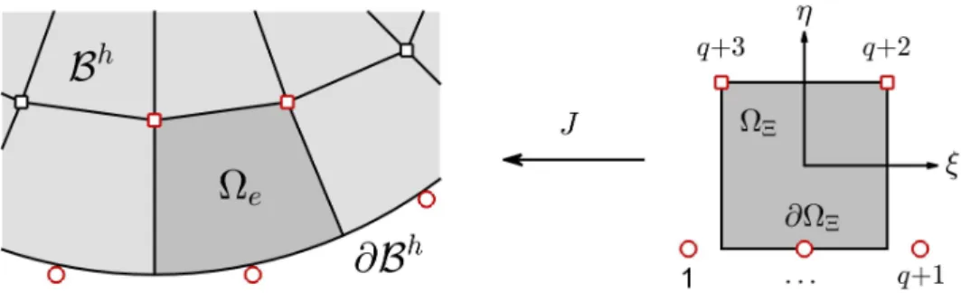
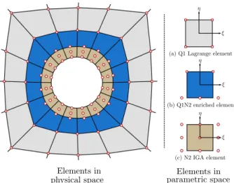
Figure 1: Isoparametric mapping between element Ωe in the physical space and element ΩΞ

in the parametric space. For the element Ωe, the control points associated with the enriched

NURBS surface are denoted by ◦ while denote standard finite element nodes.

For simplicity we first lay out the idea in a two-dimensional setting with standard linear finite elements in the bulk and NURBS enrichment of orderq at the boundary surface. Given a body

B with boundary surface∂B, consider a finite element discretizationBh _{such that}

Bh =

ne [

e=1

Ωe =Bhin∪ Bsh with Bhin∩ Bsh=∅, (29)

whereneis the total number of elements inBh_{. Elements having an edge on the surface∂B}h_are

contained inBh

s while Bhin is the set of interior elements which are devoid of any representation

of ∂B. In the finite element setting,Bh

in is represented by standard linear finite elements while

elements in Bh

s are enriched with a NURBS basis of degree q for the edge that represents ∂Bh_.

With reference to Figure 1, let us consider an element Ωe ∈ Bhs. Let J be a mapping whose

inverse transforms Ωe in the physical space to ΩΞ in the parametric space. Without loss of

generality, let us consider the edge at η =−1 in ΩΞ as the entity that represents ∂Bh for the

element Ωe. Then the enriched basis functions for such an element are given as

N1 =Rq₁(ξ) 1 2(1−η), (30) .. . Nq+1=Rqq+1(ξ) 1 2(1−η), (31) Nq+2= 1 4(1 +ξ) (1 +η), (32) Nq+3= 1 4(1−ξ) (1 +η), (33) whereRq_i are the rational basis functions defined in Eq.(25). It can be observed that the enriched basis retains the partition of unity i.e.

q+3 X

i=1

Ni(ξ, η) = 1 ∀ξ, η ∈ΩΞ, (34)

and the basis functions are always non-negative on the enriched surface

Ni(ξ,−1)≥0, withi= 1, . . . , q+ 1. (35) It is also evident that for a NURBS curve of order q = 1 and unit weights, the enriched basis functions are reduced to Lagrange polynomials of first order. Hence the 4 noded bi-linear quadrilateral element is retained in this enriched formulation as Q1N1.

Similar to the standard finite element method, we retain the concept of isoparametric elements forBh

s. This is achieved by employing, within the element, a uniform interpolation scheme for

both the geometry and the field variables, i.e.

xh= q+3 X i=1 Nixi, (36) vh= q+3 X i=1 Nivi, (37) ph = q+3 X i=1 Nipi. (38)

We employ similar basis functions for both velocity and pressure. Such an arrangement is possi-ble due to the application of PSPG stabilization scheme in Eq.(16) without which a stable pres-sure field can only be obtained by using LBB compliant elements (e.g. Taylor-Hood elements) where basis functions for velocity are usually an order higher than those for pressure. Basis functions for three dimensional enriched elements can be constructed in an analogous manner. The representative parametric element will have a bivariate NURBS surface at ζ =−1, con-nected to four interior nodes atζ = 1 through linear interpolation along theζ-direction. Hence for a NURBS surface of orderq and r, along theξ- and η-direction, we will have (q+ 1)(r+ 1) enriched basis functions and four linear Lagrange basis functions (for details see [16]).

3.3 Imposition of non-homogeneous Dirichlet boundary conditions

The imposition of Dirichlet boundary conditions presents a challenge for a spline based boundary representation. In the special case of uniform boundary conditions (i.e. when ¯v is constant in space), boundary values can be imposed exactly by collocating ¯vuniformly on the control points of the boundary surface ∂vB. However, when ¯v is not uniform and varies in space, the exact

satisfaction of Dirichlet boundary conditions is not possible due to the non-interpolatory nature of the control points. For such cases, Dirichlet boundary conditions can either be imposed weakly by incorporating them in the variational formulation [24, 57, 21] or through an approximation of ¯v based on the minimization of some error norm [17, 29]. For this study, the least square optimization technique is used to approximate ¯v for the surface∂vB.

Let us consider a velocity field v such that v = ¯v on the Dirichlet boundary ∂vB. Our goal is

to determine the values for the control variables vT_d =vT₁,vT₂, . . . ,vT_ns such that our target function Π= 1 2 X c h vh(xc)−v¯(xc) i2 (39)

is minimized. Here xc denotes a set of arbitrarily chosen points with the only requirement

that xc ∈ ∂vB. For our implementation we determine xc from the element quadrature rule.

v1,v2, . . . ,vns are control variables associated with the control points that define the boundary

surface∂vB. For a point xc, located at the surface of element e, the discrete entityvh is given

as

vh(xc) = X

i

Here the index idenotes local numbering for element e. The element shape functions and the associated control variables are contained inNe and ve such that

Ne= [N1I, N2I, . . . , NneI], (41) vT_e =

vT₁,vT₂, . . . ,vT_ne

, (42)

withne being the number of control points associated with elemente. The shape functions Ni

are evaluated at the point xc. The target function, given by Eq.(39), can be evaluated for the

elemente as Πe = 1 2 X c h Ne(xc)ve−v¯(xc) i2 . (43)

To minimize Πe, its partial derivative with respect to ve is taken and equated to zero which

leads to ∂Πe ∂ve =X c NT_e(xc) h Ne(xc)ve−v¯(xc) i =0. (44) ⇒X c NT_e(xc)Ne(xc) | {z } :=Ae ve = X c NT_e(xc) ¯v(xc). | {z } :=be (45)

Eq.(45) constitutes the normal least squares expression for the element e. Since xc spans the

entire surface∂vB,Ae andbe are constructed for every element and moved to a global system

such that "

A

A

where

A

vd=A−1b, (47)

yields control variables associated with∂vB for which the error in approximation of ¯v is mini-mized in a least squares sense. Oncevd is known, Dirichlet boundary conditions can be applied

in the same manner as usually done in a standard finite element solver. The computation ofvd

induces additional computational cost to the overall problem. However, sincevdspans only the

degrees of freedom associated with the Dirichlet boundary surface, the overhead is manageable in most cases.

4

Numerical examples

In this section we demonstrate the capabilities of isogeometrically enriched finite elements through well established numerical examples. These examples involve internal and external fluid flow around smooth curved boundaries. In the first example a three dimensional unsteady internal fluid flow, based on the Beltrami flow model, is analyzed for a spherical domain. The second example is that of a laminar fluid flow in an annular pipe which results in a steady flow field. Since analytical solutions to both these problems are known, we demonstrate the conver-gence of the error norm with respect to the exact solution through successive mesh refinement. Steady and unsteady laminar flow past a two dimensional circular cylinder, located in a rect-angular channel, constitute our final examples. The unsteady case is characterized by regular vortex shedding in the wake of the cylinder. For these examples, a comparison of important flow quantities, such as the force coefficients, is made with benchmark results.

4.1 Three dimensional Beltrami flow

An exact solution to the two-dimensional incompressible Navier–Stokes equations was formu-lated by Taylor [52] in 1923. The flow represented by this solution is known as Beltrami flow and even though such a flow may never be physically realized, the solution presents a good benchmark case for the validation of fluid flow solvers. This solution was extended by Ethier and Steinman [23] to 3D flow fields such that

p:=pex= −a2 e−2d2t 2 (e 2ax1_+e2ax2 _+e2ax3 + 2 s12c31ea(x2+x3)+ 2 s23c12ea(x3+x1)+ 2 s31c23ea(x1+x2)) , (48) v:=vex=−a e−d 2_t   s23eax1+ c12ea x3 s31eax2+ c23ea x1 s12eax3+ c31ea x2   (49)

is an exact solution of the dimensionless Navier–Stokes equations. Here

sij := sin (a xi+d xj) and cij := cos (a xi+d xj), (50)

whereaand dare constants whose values can be chosen arbitrarily. Under the current setting,

a=π_{/4 and d=} π_{/2. We consider a fluid domain B. For our test caseB takes the shape of a}

solid sphere of unit radius while the surface of the sphere ∂Bs constitutes the boundary of the

domain. The problem is set up with purely Dirichlet boundary conditions such that

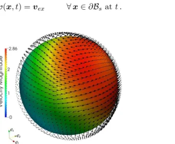
v(x, t) =vex ∀x∈∂Bs att . (51)

Figure 2: Beltrami flow: Contours of non-dimensional velocity v with velocity vectors on ∂Bs

att= 0.

Figure 2 depicts the imposed velocity on the boundary surface ∂B_s at the start of the compu-tations. The reference pressure is set by specifying pex at the node closest to the center of the

sphere. A time interval of [0,10] is used. Two cases, based on the discretization of the boundary surface ∂B_s, are considered. In the first case, B is discretized entirely with Lagrangian finite elements of first order (Q1N1). For brevity, we drop the extended notation for these elements and denote them as Q1. This discretization is referred as the pure Q1 discretization. The second case, denoted as the surface enriched discretization, comprises a discretization where the elements having a face on ∂Bs are enriched with a B-spline surface of second order (i.e. Q1N2

elements). This results in an approximation of the spherical boundary surface ∂Bs which is

completelyC1-continuous. L2-Error norms with respect to the exact solution, i.e.

ev(vh, t) = ||vex−vh||2 ||vex||2 , (52) ep(ph, t) = ||pex−p h_|| 2 ||pex||2 (53)

are computed and studied for a series of uniformly refined meshes. Here v is the velocity magnitude, i.e.

v=

q

v2₁+v₂2+v2₃, (54)

while || · ||₂ is the L2-norm which is given as

|| · ||2= s

Z

B

(·)2 _{dV . (55)}

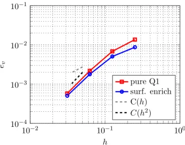
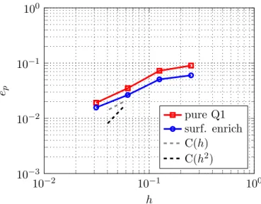
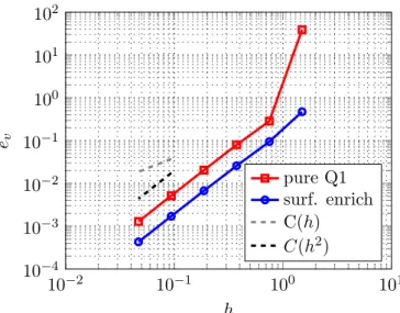
Results for the mesh convergence study for error normsevandepatt= 10 are shown in Figure3

and Figure 4. Here h denotes the average element length in Bh_{. It can be observed that the}

discrete solution tends to approach the exact solution as the mesh is refined. If the convergence behavior of the pure Q1 discretization is compared with the surface enriched discretization, it becomes evident that the gain in accuracy, due to the enrichment of surface with B-splines, is not substantial. This behavior can be attributed to the unbounded nature of the Beltrami flow solution given by Eq.(48) and Eq.(49). The solution holds true for all x ⊂ _R3 _{and is}

not influenced by the shape of the boundary surface ∂B_s. Hence, the gain in accuracy due to a better approximation of the spherical boundary surface ∂Bs is not significant and only an

improvement in the interpolation error is observed.

10−2 ₁₀−1 ₁₀0 10−4 10−3 10−2 10−1 h ev pure Q1 surf. enrich C(h) C(h2)

Figure 3: Beltrami flow: Convergence of the velocity error norm ev with mesh refinement for the Beltrami flow case at t= 10 s.

4.2 Laminar flow in an annular pipe

The fluid flow between two concentric cylinders of different radii is considered in this example. The problem presents an exact solution to the governing Navier Stokes equations, provided the

10−2 10−1 100 10−3 10−2 10−1 100 h ep pure Q1 surf. enrich C(h) C(h2)

Figure 4: Beltrami flow: Convergence of the pressure error norm ep with mesh refinement for

the Beltrami flow case at t= 10 s.

flow remains laminar. It has been observed that for a Reynolds number<2000, the fluid flow in circular pipes is predominantly laminar [44]. For annular pipes, the non-dimensional quantity Reynolds number is defined as

ReH = ρvDH¯

µ , (56)

where DH is the hydraulic diameter of the pipe such that DH = 2Ro−2Ri and ¯v is the bulk (average) velocity. The terms Ro and Ri denote the radii of the outer and the inner cylinder respectively. If the axis of the pipe is aligned alonge2, then for laminar flow regimes the velocity

of the fluid in the pipe is given as

v2 = 1 4ν − dp dx2 R_o2−R2+ R 2 o−R2i ln(Ri/Ro)ln Ro R , (57)

with v1 =v3 = 0 [56,41]. Here the term dp/dx2 denotes the pressure gradient along the axial

direction while R denotes the radial distance from the axis of the pipe.

Refinement Elements Nodes + Control points

Pure Q1 Surf. enrich Pure Q1 Surf. enrich

Q1 Q1 Q1N2 Coarsest 8 – 8 24 32 1st 32 16 16 80 96 2nd 128 96 32 288 320 3rd 512 448 64 1088 1152 4th 2048 1920 128 4224 4352 5th 8192 7936 256 16,640 16,896

Table 1: Annular pipe flow: Element and nodal density data for successive spatial mesh refine-ments.

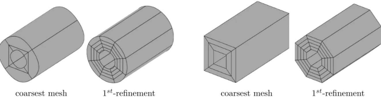
discretiza-coarsest mesh 1st_{-refinement coarsest mesh 1}st_-refinement

Figure 5: Annular pipe flow: Two successive spatial meshes - surface enriched discretizations are shown on the left while pure Q1 discretizations are given on the right.

boundaries while the inlet and outlet faces are modeled as periodic boundaries. For the surface enriched discretization, B-spline surfaces of second order (i.e q=r = 2) were used to represent the surface of the cylinders. The flow in the pipe is driven by a uniform pressure gradient which is applied as a constant forceb= (0, b2,0) in the axial direction.

0 50 100 150 200 250 300 350 10−4 10−3 10−2 ReH ev pure Q1 surf. enrich

Figure 6: Annular pipe flow: Behavior of the velocity error norm ev at different ReH.

Computations are performed on a series of meshes which are uniformly refined along the radial and circumferential direction. The error norm for velocity magnitudeev (defined in Eq.(52)) is

computed at differentReH and mesh convergence is analyzed.

Figure 6 shows the behavior of ev at different ReH(14,30,100 and 300) for the finest spatial mesh. It can be observed that within the laminar flow regime, the error in the solution field is independent ofReH. Hence, convergence analysis is performed for onlyReH = 100 subsequently. The convergence behavior for the two discretizations is shown in Figure7. It is evident that the surface enriched discretization approximates the solution with higher accuracy (approximately by a factor of 3) as compared to Lagrangian finite elements, especially at the coarsest level. The optimal rate of convergence is dictated primarily by the Q1 elements present in the bulk and hence is comparable to second order for theL2-error norm. An illustration for the absolute error in the velocity field is provided in Figure8. It can be observed from the figure that for the pure Q1 discretization maximum error occurs at regions where the error in the approximation of the cylinder radii is large. Hence an improved approximation of the cylindrical surface due to Q1N2 elements lead to a significantly improved solution.

10−2 10−1 100 101 10−4 10−3 10−2 10−1 100 101 102 h ev pure Q1 surf. enrich C(h) C(h2)

Figure 7: Annular pipe flow: Convergence of the velocity error norm ev with mesh refinement.

Figure 8: Annular pipe flow: Contours of the relative error in the velocity field at ReH = 100

for the surface enriched discretization (left) and the pure Q1 discretization (right) at the 1st -refinement.

4.3 Flow around a cylinder

A set of problems were defined by Turek and Sch¨afer [55] for establishing benchmark results for validating flow solvers. These are composed of benchmark cases involving laminar fluid flow around a stationary rigid cylinder (2D and 3D) of uniform cross-section enclosed in a rectangular channel. In this example, the benchmark cases for the steady and the unsteady laminar flow past a two-dimensional circular cylinder (denoted as 2D-1 and 2D-3 in [55]) are considered.

Let us consider a fluid domainB which consists of a rectangular channel with a stationary rigid cylinder. Figure 9 provides an illustration of the domain and its associated dimensions. The boundary of the domain ∂B comprises the surface of the cylinder, the inlet, the outlet and the

Figure 9: Flow around a cylinder: Flow domain with associated dimensions as defined in [55]

channel walls. The following boundary conditions are associated with the problem:

v= (v1,0) ∀x∈∂Bin, (58)

v=0 ∀x∈∂B\(∂Bin∪∂Bout) , (59)

σ·n=0 ∀x∈∂Bout, (60)

where∂Bin represents the inlet boundary (atx1= 0) while∂Bout denotes the outlet boundary

(at x1 = 2.2 m). A fluid of density 1.0 kg/m3 and a kinematic viscosity ν = 10−3 m2/s is

considered. The Reynolds number for this example is defined as

Re= ρ¯v1D

µ , (61)

where D = 2r , is the diameter of cylinder and ¯v1 is the average inlet velocity which is given

as ¯ v1 = 1 H Z H 0 v1(0, x2, t) dx2, (62)

with H being the height of the channel. Non-dimensional force coefficients for the drag force

Cd and the lift force Cl have been reported for these benchmark problems. These are defined

as Cd= f1 1 2ρv¯12D , (63) Cl= f2 1 2ρv¯12D . (64)

Here f = (f1, f2) is the force exerted by the fluid on the cylinder which is given by

f =

Z

∂Bc

σ·ndS , (65)

where∂B_crepresents the surface of the cylinder.

In terms of discretization, four cases are considered for this benchmark problem. The first one consists of a spatial discretization composed entirely of Lagrangian finite elements of first order. The second case uses a spatial discretization where the elements, that have a face on the cylinder, are enriched with a second order B-spline based surface description. This results in an approximation of the cylindrical surface which is completelyC1-continuous. These cases,

similar to previous examples, are denoted as the pure Q1 discretization and the surface enriched discretization respectively. Furthermore, a new discretization is introduced in which the mesh in the immediate vicinity of the cylinder is enriched with elements having B-spline based volumetric representation. Such elements have been the standard choice in IGA (see [17]). In this text they are referred as IGA elements and, as per the earlier defined nomenclature in this paper, can be denoted as NqNr. Such an enrichment is motivated by considering the impact of the boundary layer resolution on the overall flow field. It is assumed that the flow field can be captured with higher accuracy by not only enriching the surface of the cylinder, but by also enriching the area in the immediate vicinity of the cylinder where the boundary layer develops and strong gradients in the field variables arise. We refer to this discretization as the zone enriched discretization. For this example IGA elements of uniform order in all directions, i.e. q = r, are considered. Therefore they are simply denoted as Nq in the following discussion. Since the boundary layer exists only in the immediate vicinity of the cylinder, therefore the thicknesstof the purely IGA enriched region can be kept small. Here t≈0.5r. A representation of the zone enriched case with N2 elements is depicted in Figure 10. The fourth case comprises a domain, discretized entirely with Nq IGA elements, yielding the highest degrees of freedom among the four cases. This is referred to as the pure IGA case. Table2summarizes the element densities while Table3

lists the nodal densities associated with the different discretization cases.

Figure 10: Flow around a cylinder: Enrichment of the boundary layer around the cylinder with N2 IGA elements. The Q1N2 surface enriched elements are used to interface IGA with standard FEA.

Refinement Elements

Pure Q1 Surf. enrich Zone enrich Pure IGA

Q1 Q1 Q1N2 Q1 Q1N2 N2 N2 Coarsest 128 112 16 96 16 16 128 1st 512 480 32 416 32 64 512 2nd 2048 1984 64 1728 64 256 2048 3rd 8192 8064 128 7040 128 1024 8192 4th 32,768 32,512 256 28,416 256 4096 32,768 5th 131,072 130,560 512 114,176 512 16,384 131,072

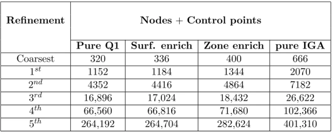
Refinement Nodes +Control points

Pure Q1 Surf. enrich Zone enrich pure IGA

Coarsest 320 336 400 666 1st 1152 1184 1344 2070 2nd 4352 4416 4864 7182 3rd 16,896 17,024 18,432 26,622 4th 66,560 66,816 71,680 102,366 5th 264,192 264,704 282,624 401,310

Table 3: Flow around a cylinder: Nodal density data for successive spatial mesh refinements.

4.3.1 Steady flow (Re= 20)

The first test case (denoted as 2D-1 in [55]) considers a parabolic velocity profile

v1(0, x2) =

4vmx2

H2 (H−x2) (66)

prescribed at the inlet. With vm= 0.3 m/s, a Reynolds number of 20 is obtained.

The problem is analyzed for successively refined meshes. The behavior of the relative error in the drag coefficient Cd is shown in Figure 11. Cdh represents the value obtained from the

current analysis, while C_dref refers to the reference drag coefficient from which the relative error is computed. In [42], reference values for this benchmark problem were computed using higher-order spectral methods. It can be observed from the plot that C_dh tends to approach the reference solution as the mesh is refined. Moreover, it can also be inferred that the surface enriched discretization is comparatively more accurate than the pure Q1 case. Although the gain in accuracy is not significant for the surface enriched discretization, a substantial gain in accuracy is observed for the zone enriched case when IGA volume elements are added in the immediate vicinity of the cylinder. This is accompanied by an improvement in the convergence rate as well. The zone enriched discretization approaches the reference solution with second order convergence, while the convergence rates for the other two discretizations are comparable to first order. Hence the assumption, that a better capturing of the boundary layer by IGA elements will yield a more accurate flow field, is validated. The pure IGA case, as expected, yields the most accurate solution for the same level of refinement.

A comparative analysis of the results presented in Figure 11 reflects the performance of each discretization. When compared with the pure Q1 and the surface enriched case, it can be ob-served that a coarse discretization of the pure IGA case (e.g. 2nd-refinement) yields an accuracy that is comparable to a much finer discretization of the other two cases (4th-refinement). This behavior has been reported previously in [7,40]. However the convergence rate and the error norms for the zone enriched case are comparable to those obtained for the pure IGA case, while at the same time the associated degrees of freedom ndof are significantly less. To quantify this

behavior, relative measures for cost and accuracy are computed for the zone enriched and the pure IGA cases in relation to the pure Q1 results. The relative increment in the computational cost is assessed by δ(_cost·) = n (·) dof−n (Q1) dof n(Q1)_dof , (67)

whereas the relative gain in accuracy (reduction in error) is computed as δ_acc(·) = E (Q1) d −E (·) d E_d(Q1) . (68)

The superscript represent the discretization case being considered whileEdis measured as

Ed=

|C_dref −C_dh|

C_dref . (69)

The results of these measures are tabulated in Table 4. At the finest level, the pure IGA case results in a 92.8% relative improvement in accuracy in relation to the pure Q1 discretization. However, this improvement is attained at a significant cost of 53.8%. On the other hand, the zone enriched case yields an improvement of 86.7% with only a 7.7% increment in ndof.

Convergence plots for the lift coefficient and the pressure difference at the two given reference points are shown in Figure 12 and Figure13.

Refinement Zone enrich Pure IGA

δ_cost(zone) δacc(zone) δcost(IGA) δ (IGA) acc (%) (%) (%) (%) 1st 16.7 62.6 79.7 68.8 2nd 11.8 70.2 65.0 80.2 3rd 9.1 78.5 57.6 88.0 4th 7.7 86.7 53.8 92.8

Table 4: Flow around a cylinder: Comparison of the rise inndof vs. gain in accuracy.

10−3 10−2 10−1 100 10−4 10−3 10−2 10−1 100 h | C r ef d − C h|d C r ef d pure Q1 surf. enrich zone enrich pure IGA C(h) C(h2)

Figure 11: Steady flow around a cylinder: Relative error in the computed drag force coefficient

10−3 10−2 10−1 100 10−4 10−3 10−2 10−1 100 101 h | C r ef l − C h|l C r ef l _{pure Q1} surf. enrich zone enrich pure IGA C(h) C(h2₎

Figure 12: Steady flow around a cylinder: Relative error in the lift force coefficientC_lhin relation to the reference valueC_lref [42].

10−3 10−2 10−1 100 10−4 10−3 10−2 10−1 100 h | ∆ p r ef − ∆ p h| ∆ p r ef pure Q1 surf. enrich zone enrich pure IGA C(h) C(h2₎

Figure 13: Steady flow around a cylinder: Relative error in the pressure difference ∆ph in relation to the reference value ∆pref [42].

4.3.2 Unsteady flow 0≤Re≤100

The flow in this regime corresponds to the 2D-3 benchmark case in [55]. The inflow velocity is given as

v1(0, x2, t) =

4vmx2

H2 (H−x2) sin (πt/8) (70)

where vm is taken to be 1.5 m/s. A time interval t ∈ [0,8 s] is chosen. This results in a flow regime, which builds from Re= 0 to a maximum Re= 100 at t= 4 s and then decays back to the initial condition.

The inflow conditions given by Eq.(70) leads to a time-dependent flow fluid. To integrate Eq.(15) and Eq.(16) over time, we use the generalized α-method. It was first presented in [11] and later applied to the Navier–Stokes equations in [36]. For this benchmark problem, successive

refinements in spatial as well as temporal discretization are considered. Table5summarizes the spatial mesh data together with the associated time-step size (∆t).

Refinement Elements ∆t (s) Coarsest 128 0.05 1st 512 0.02 2st 2048 0.01 3rd 8192 0.005 4th 32,768 0.0025

Table 5: Unsteady flow around a cylinder: Spatial and temporal data for successive refinements.

Reference data from [1] is used to benchmark the numerical results for this problem. In [1],

Cd and Cl were computed over successively refined spatial meshes comprising of Taylor-Hood

(Q2/P1) quad finite elements. We choose the finest available resolution (i.e. 133,120 elements

and ∆t= 1/1600 s) as our reference solution. In order to evaluate the relative error in the force coefficients over the entire time scale, the following error norms are considered:

ed= v u u u u t P t C_dref −C_dh2 P t C_dref2 , (71) el = v u u u u t P t C_lref −Ch l 2 P t C_lref2 (72)

where the summation is performed over all time-steps int.

10−3 10−2 10−1 100 10−4 10−3 10−2 10−1 100 h ed pure Q1 surf. enrich zone enrich C(h) C(h2)

Figure 14: Unsteady flow around a cylinder: Error norm (ed) for successive spatial and temporal

refinements.

Figure 14 and Figure 15 depict the behavior of the error norms ed and el respectively, over

successive refinements in space and time. It can be inferred from Figure 15 that the initial

10−3 10−2 10−1 100 10−2 10−1 100 101 h el pure Q1 surf. enrich zone enrich C(h) C(h2)

Figure 15: Unsteady flow around a cylinder: Error norm (el) for successive spatial and temporal

refinements.

approximation of the flow field since the values ofelare large and the behavior is not consistent. As the spatial and temporal resolution is improved, el decreases and the behavior becomes

consistent with the previous observations. For sufficiently refined resolutions, it can be observed that the addition of N2 IGA elements, in the immediate vicinity of the cylinder, results in a more accurate solution. Fluid flow past a stationary cylinder atRe >40 is usually characterized by vortex shedding in the wake of the cylinder. For such flow regimes, localized enrichment only in the boundary layer region is not entirely sufficient and the spatial mesh in the wake region should also be sufficiently improved to accurately resolve the vortices traveling in the wake region. This can be achieved either by refining the Q1 finite elements in the wake region or by extending the enrichment zone to include the wake region. When applied to a structured spatial mesh, the first strategy will add refined Q1 finite elements in the beyond-wake region as well since refinement lines have to be translated throughout the entire domain. This will subsequently increase the computational cost of the analysis by many folds. A localized IGA enrichment, on the other hand, will only influence the spatial mesh in the wake region and will increase the computational cost marginally.

5

Conclusion and outlook

In this paper, we extend the applicability of the isogeometrically enriched finite element method to problems involving incompressible laminar flow. It is successfully demonstrated that the tech-nique results in a more accurate method as compared to standard finite element discretization. This is achieved by an enriched representation of the underlying surface geometry, which is at leastC1-continuous, in conjunction with high-order evaluation of both the surface and the vol-ume integrals by an enriched basis. At the same time, the cost associated with the enrichment is kept to a minimum by performing a highly localized enrichment. Such a methodology is extremely useful in fluid flow problems where often the overall fluid domain is extremely large as compared to the region of interest. Moreover, together with surface enrichment, the possi-bility of interfacing IGA with standard finite elements through Q1Nq elements is also explored. For our model problems, a significant gain in accuracy and convergence rate is observed when localized NURBS based enrichment is performed in a volumetric setting in the boundary layer

region. Thus the premise, that effective modeling of gradients associated with the boundary layer might lead to a better solution, stands validated.

The isogeometrically enriched finite element method provides additional benefits in terms of mesh generation when compared with IGA. In practice, it is often only the surface description that is available from a CAD software and fitting a complete IGA base spatial mesh to the entire domain is usually a cumbersome task. By using isogeometrically enriched finite elements, a CAD based IGA surface mesh can be blended to a standard finite element mesh with relative ease, even for complex geometries as demonstrated in [16]. Hence the novel technique presented in this work can be effectively employed for IGA based localized enrichment of important regions of the flow domain, resulting in a strategy which is efficient and accurate.

We believe that an extension of the proposed enrichment strategy to turbulent flow analysis, where the boundary layer tends to diminish and surface gradients are particularly strong, will further establish the merits of this approach. The superior accuracy of IGA for turbulent flow analysis is a well established fact (see [4,41]) and the proposed strategy retains the character of IGA at the enriched zones. If applied intelligently to turbulent flow problems, the enrichment has the potential of yielding an accuracy similar to IGA at a cost similar to Lagrangian finite elements.

Acknowledgments

References

[1] Featflow Benchmark Suite. http://www.featflow.de/en/benchmarks/ cfdbenchmarking/flow.html, March 2015.

[2] I. Akkerman, Y. Bazilevs, V. M. Calo, T. J. R. Hughes, and S. Hulshoff. The role of continuity in residual-based variational multiscale modeling of turbulence. Computational Mechanics, 41(3):371–378, 2008.

[3] C. Baiocchi, F. Brezzi, and L. P. Franca. Virtual bubbles and the Galerkin least-squares method. Computer Methods in Applied Mechanics and Engineering, 105:125–141, 1993.

[4] Y. Bazilevs, V. M. Calo, J. A. Cottrell, T. J. R. Hughes, A. Reali, and G. Scovazzi. Vari-ational multiscale residual-based turbulence modeling for large eddy simulation of incom-pressible flows. Computer Methods in Applied Mechanics and Engineering, 197(1-4):173– 201, 2007.

[5] Y. Bazilevs, C. Michler, V. M. Calo, and T. J. R. Hughes. Isogeometric variational multi-scale modeling of wall-bounded turbulent flows with weakly enforced boundary conditions on unstretched meshes. Computer Methods in Applied Mechanics and Engineering, 199(13-16):780–790, 2010.

[6] T. Belytschko and T. Black. Elastic crack growth in finite elements with minimal remeshing.

[7] D. J. Benson, Y. Bazilevs, E. De Luycker, M.-C. Hsu, M. Scott, T. J. R. Hughes, and T. Belytschko. A generalized finite element formulation for arbitrary basis functions: From isogeometric analysis to XFEM.International Journal for Numerical Methods in Engineer-ing, 83(6):765–785, 2010.

[8] M. J. Borden, M. A. Scott, J. A. Evans, and T. J. R. Hughes. Isogeometric finite element data structures based on B´ezier extraction of NURBS.International Journal for Numerical Methods in Engineering, 87:15–47, 2011.

[9] A. N. Brooks and T. J. R. Hughes. Streamline Upwind/Petrov-Galerkin formulations for convection dominated flows with particular emphasis on the incompressible Navier-Stokes equations. Advances in Applied Mechanics, 32:199–259, 1982.

[10] A. J. Chorin. A numerical method for solving incompressible viscous flow problems.Journal of Computational Physics, 135:118–125, 1997.

[11] J. Chung and G. M. Hulbert. A time integration algorithm for structural dynamics with improved numerical dissipation: the generalized-α method. Journal of Applied Mechanics, 60:371–375, 1993.

[12] R. Codina. Comparison of some finite element methods for solving the diffusion-convection-reaction equations. Computer Methods in Applied Mechanics and Engineering, 156:185– 210, 1998.

[13] N. Collier, L. Dalcin, D. Pardo, and V. M. Calo. The cost of continuity: performance of iterative solvers on isogeometric finite element. SIAM Journal on Scientific Computing, 35(2):A767–A784, 2013.

[14] N. Collier, D. Pardo, L. Dalcin, M. Paszynski, and V. M. Calo. The cost of continuity: A study of the performance of isogeometric finite elements using direct solvers. Computer Methods in Applied Mechanics and Engineering, 213-216:353–361, 2012.

[15] C. J. Corbett and R. A. Sauer. NURBS-enriched contact finite elements.Computer Methods in Applied Mechanics and Engineering, 275:55–75, 2014.

[16] C. J. Corbett and R. A. Sauer. Three-dimensional isogeometrically enriched finite elements for frictional contact and mixed-mode debonding.Computer Methods in Applied Mechanics and Engineering, 284:781–806, 2015. Isogeometric Analysis Special Issue.

[17] J. A. Cottrell, T. J. R. Hughes, and Y. Bazilevs.Isogeometric Analysis: Toward Integration of CAD and FEA. John Wiley & Sons, 2009.

[18] M. G. Cox. The numerical evaluation of B-splines. IMA Journal of Applied Mathematics, 10:134–149, 1971.

[19] C. de Boor. On calculating with B-splines. Journal of Approximation Theory, 6:50–62, 1972.

[20] J. Donea and A. Huerta. Finite Element Methods for Flow Problems. John Wiley & Sons, 2003.

[21] A. Embar, J. Dolbow, and I. Harari. Imposing Dirichlet boundary conditions with Nitsche’s method and spline based finite elements. International Journal for Numerical Methods in Engineering, 83:877–898, 2010.

[22] I. Ergatoudis, B. Irons, and O. C. Zienkiewicz. Curved, isoparametric, “quadrilateral” elements for finite element analysis. International Journal of Solids and Structures, 4:31– 42, 1968.

[23] C. R. Ethier and D. A. Steinman. Exact fully 3D Navier-Stokes solutions for benchmarking.

International Journal for Numerical Methods in Fluids, 19:369–375, 1994.

[24] S. Fern´andez-M´endez and A. Heurta. Imposing essential boundary conditions in mesh-free methods.Computers Methods in Applied Mechanics and Engineering, 193:1257–1275, 2004. [25] J. Floryan and H. Rasmussen. Numerical methods for viscous flow with moving boundaries.

Applied Mechanics Reviews, 42:323–341, 1989.

[26] L. P. Franca and F. Valentin. On an improved unusual stabilized finite element method for the advective-reactive-diffusive equation. Computer Methods in Applied Mechanics and Engineering, 190:1785–1800, 2000.

[27] P. Gamnitzer, V. Gravemeier, and W. A. Wall. Time-dependent subgrid scales in residual-based large eddy simulation of turbulent channel flow. Computer Methods in Applied Mechanics and Engineering, 199(13-16):819–827, 2010.

[28] W. J. Gordon and C. A. Hall. Transfinite element methods: Blending-function interpolation over arbitrary curved element domains. Numerische Mathematik, 21:109–129, 1973.

[29] S. Govindjee, J. Strain, T. J. Mitchell, and R. L. Taylor. Convergence of an efficient local Least-Squares fitting method for bases with compact support.Computer Method in Applied Mechanics and Engineering, 213-216:84–92, 2012.

[30] P. M. Gresho and R. L. Sani. Incompressible Flow and the Finite Element Method. Wiley, 1998.

[31] I. Harari and T. J. R. Hughes. What arecand h?: Inequalities for the analysis and design of finite element methods. Computer Methods in Applied Mechanics and Engineering, 97:157–192, 1992.

[32] F. H. Harlow and E. Welch. Numerical calculation of time-dependent viscous incompressible flow of fluids with free surface. Physics of Fluids, 8:2182–2189, 1965.

[33] L. P. F. G. Hauke and A. Masud. Revisiting stabilized finite element methods for the advective-diffusive equation. Computer Methods in Applied Mechanics and Engineering, 195:1560–1572, 2006.

[34] T. J. R. Hughes. Multiscale phenomena: Green’s function, the Dirichlet-to-Neumann formulation, subgrid scale models, bubbles and origins of stabilized methods. Computer Methods in Applied Mechanics and Engineering, 127:387–401, 1995.

[35] T. J. R. Hughes, J. A. Cottrell, and Y. Bazilevs. Isogeometric Analysis: CAD, finite elements, NURBS, exact geometry and mesh refinement. Computer Methods in Applied Mechanics and Engineering, 194:4135–4195, 2005.

[36] K. E. Jansen, C. H. Whiting, and G. M. Hulbert. A generalized-α method for integrating the filtered Navier-Stokes equations with a stabilized finite element method. Computer Methods in Applied Mechanics and Engineering, 190:305–319, 1999.

[37] C. Kiris and D. Kwak. Numerical solution of incompressible Navier-Stokes equations using a fractional-step approach. InAIAA Paper 96-2089, 27th AIAA Fluid Dynamics Conference,

[38] P. Knaber and L. Angermann. Numerik partieller Differentialgleichungen. Eine anwen-dungsorientierte Einf¨uhrung. Springer, 2000.

[39] B. Koobus and C. Farhat. A variational multiscale method for the large eddy simulation of compressible turbulent flows on unstructured meshes—application to vortex shedding.

Computer Methods in Applied Mechanics and Engineering, 193(15-16):1367–1383, 2004. [40] S. Morganti, F. Auricchio, D. J. Benson, F. I. Gambarin, S. Hartmann, T. J. R. Hughes, and

A. Reali. Patient-specific isogeometric structural analysis of aortic valve closure.Computer Methods in Applied Mechanics and Engineering, 284:508–520, 2015. Isogeometric Analysis Special Issue.

[41] Y. G. Motlagh, H. T. Ahn, T. J. R. Hughes, and V. M. Calo. Simulation of laminar and turbulent concentric pipe flows with the isogeometric multiscale method. Computers & Fluids, 71:146–155, 2013.

[42] G. Nabh. On higher order methods for the stationary incompressible Navier-Stokes equa-tions. PhD thesis, Universit¨at Heidelberg, 1998.

[43] L. Piegel and W. Tiller. The NURBS Book. Springer, 1997.

[44] O. Reynolds. An experimental investigation of the circumstances which determine whether the motion of water shall be direct or sinuous and the law of resistance in parallel channels.

Philosophical Transactions of the Royal Society of London, 174:935–982, 1883.

[45] S. E. Rogers, D. Kwak, and C. Kiris. Steady and unsteady solutions of the incompressible Navier-Stokes equations. AIAA Journal, 29:603–610, 1991.

[46] M. Rosenfeld, D. Kwak, and M. Vinokur. A solution method for unsteady, incompressible Navier–Stokes equations in generalized curvilinear coordinate systems. Journal of Compu-tational Physics, 94:102–137, 1991.

[47] R. A. Sauer. Enriched contact finite elements for stable peeling computations.International Journal for Numerical Methods in Engineering, 87:593–616, 2011.

[48] R. A. Sauer. Local finite element enrichment strategies for 2D contact computations and a corresponding postprocessing scheme. Computational Mechanics, 52:301–319, 2013.

[49] R. Sevilla, S. Fernandez-Mendez, and A. Huerta. NURBS-enhanced finite element method (NEFEM). International Journal for Numerical Methods in Engineering, 76:56–83, 2008.

[50] F. Shakib. Finite element analysis of the incompressible Euler and Navier-Stokes equa-tions. PhD thesis, Department of Mechanical Engineering, Stanford University, Stanford, California, 1988.

[51] W. Shyy, H. Udaykumar, M. M. Rao, and R. W. Smith. Computational Fluid Dynamics with Moving Boundaries. Taylor & Francis, 1996.

[52] G. I. Taylor. On the decay of vortices in a viscous fluid. Philosophical Magazine Series 6, 46:671–674, 1923.

[53] T. E. Tezduyar. Stabilized finite element formulations for incompressible flow computations.

Advances in Applied Mechanics, 28:1–44, 1992.

[54] T. E. Tezduyar. Interface-tracking and interface-capturing techniques for finite element computation of moving boundaries and interfaces.Computer Methods in Applied Mechanics and Engineering, 195:2983–3000, 2006.

[55] S. Turek and M. Sch¨afer. Benchmark computations of laminar flow around cylinder. In E. Hirschel, editor, Flow Simulation with High-Performance Computers II, volume 52 of

Notes on Numerical Fluid Mechanics, pages 547–566. Vieweg, Jan. 1996.

[56] F. M. White. Fluid Mechanics. McGraw-Hill, fourth edition, 2003.

[57] T. Zhu and S. N. Atluri. A modified collocation method and a penalty formulation for enforcing the essential boundary conditions in the element free Galerkin method. Compu-tational Mechanics, 21:211–222, 1998.

[58] M. Zlamal. Curved elements in the finite element method. I. SIAM Journal on Numerical Analysis, 10:229–240, 1973.