Federal Reserve Bank of New York
Staff Reports
This paper presents preliminary fi ndings and is being distributed to economists and other interested readers solely to stimulate discussion and elicit comments. The views expressed in this paper are those of the authors and are not necessarily refl ective of views at the Federal Reserve Bank of New York or the Federal Reserve System. Any errors or omissions are the responsibility of the authors.
Staff Report No. 551
February 2012
Matthew Denes
Gauti B. Eggertsson
Sophia Gilbukh
Denes: University of Pennsylvania. Eggertsson, Gilbukh: Federal Reserve Bank of New York (e-mail: gauti.eggertsson@ny.frb.org, sophia.gilbukh@ny.frb.org). The views expressed in this paper are those of the authors and do not necessarily refl ect the position of the Federal Reserve
Abstract
Cutting government spending on goods and services increases the budget defi cit if the nominal interest rate is close to zero. This is the message of a simple but standard New Keynesian DSGE model calibrated with Bayesian methods. The cut in spending reduces output and thus—holding rates for labor and sales taxes constant—reduces revenues by even more than what is saved by the spending cut. Similarly, increasing sales taxes can increase the budget defi cit rather than reduce it. Both results suggest limitations of “aus-terity measures” in low interest rate economies to cut budget defi cits. Running budget defi cits can by itself be either expansionary or contractionary for output, depending on how defi cits interact with expectations about the long run in the model. If defi cits trigger expectations of i) lower long-run government spending, ii) higher long-run sales taxes, or iii) higher future infl ation, they are expansionary. If defi cits trigger expectations of higher long-run labor taxes or lower long-run productivity, they are contractionary.
Key words: fi scal policy, liquidity trap
Defi cits, Public Debt Dynamics, and Tax and Spending Multipliers Matthew Denes, Gauti B. Eggertsson, and Sophia Gilbukh
Federal Reserve Bank of New York Staff Reports, no. 551 February 2012
1
Introduction
When the world economic crisis hit in 2008, several of the world’s leading central banks cut the short-term nominal interest rate close to zero. Most governments, however, responded by implementing somewhat expansionaryfiscal policies, although there is some controversy over how expansionary they actually were. Meanwhile, budget deficits ballooned in most countries, mostly due to the collapse in the tax base following the recession. Although most private forecasters expected a robust recovery in 2009 and 2010, it turned out to be very sluggish. At that time, by most accounts, the economic discussion became centered on how to balance the government budget and the focus shifted from recovery via interest rate cuts and deficit spending to "austerity measures." As of this writing, economic recovery remains uncertain, and to the contrary of an improving in fiscal situation, some parts of the world are faced by ever expanding budget deficits, and in some cases even serious concerns of outright default of the sovereign.
The goal of this paper is to analyze debt dynamics in a standard New Keynesian dynamic stochastic general equilibrium (DSGE) model in a low interest rate environment. One of our mainfindings is that the rules for budget management change once the short-term nominal interest rate approaches zero. This shows up in our model in at least two ways. First, we show that once the short-term nominal interest rate hits zero, then cutting government spending or raising sales taxes increases rather than reduces the budget deficit. This is in contrast to the marginal effects of both policies under normal circumstances when they reduce the deficit. Second, we find that the economy is extraordinary sensitive to expectations about long-run policy at zero interest rates. In particular, expectations about the future size of the government and future sales and labor taxes can have strong effects on short-run demand. This is again in contrast to an economy where the nominal interest rate is positive and the central bank targets zero inflation. In that environment we show that long-run expectations are completely irrelevant in the model. An important implication of this is that in low interest rate environment budget deficits can either increase or reduce aggregate demand in the short-run, depending on how they influence expectations of future taxes, spending, and monetary policy. Hence the effect of deficit spending at zero interest ratedepends critically on the policy regime. Below we outline the organization of the paper and elaborate on each of these points in turn.
After laying out and parameterizing the model (Section 2) we first confront it (Section 3) with the following thought experiment: Suppose there are economic conditions such that the nominal interest rate is close to zero and the central bank wants to cut rates further, but
cannot. Suppose sale and labor tax rates are held constant. How does the budget deficit react if the government tries to balance the budget by cutting government spending, i.e. via "austerity measures" popular in many countries in reaction to the budget deficits stemming from crisis of 2008? The model suggests that under reasonable parameters, the budget deficit increases rather than decreases. This occurs because the cut in government spending leads to a reduction in aggregate output, thus reducing the tax base and subsequently reducing tax revenues. Our result is thus akin to being on the "wrong" side of the famous "Laffer curve" where cutting tax rates increases revenues by increasing the tax base. Here we see, instead, that cutting government expenditures can increase the deficit due to the shrinking of the tax base, so that even if the government is now spending less, the amount of money it collects via taxes drops by even more. We derive simple analytical conditions under which this applies. Conducting the same experiment with sales taxes we obtain a similar result: There is also a simple condition under which increasing sales taxes reduces tax revenues and we show that this is particularly likely to happen once there are shocks that make the zero bound binding. To the keen observer of the current economic turmoil, then, it may seem somewhat disturbing that expenditure cuts and sale tax increases were two quite popular policies in response to the deficits following the crisis of 2008.
While the first set of results points against the popular call for "austerity," we have a second set of results that puts these calls, perhaps, in a bit more sympathetic light. We next consider (Section 4) the following question: How does demand in the short-run react to expectations about long-run taxes, long-run productivity and the long-run size of the government? One motivation for this question is that we often hear discussion about the importance of "confidence" in the current economic environment and this is given as one rationale for reducing deficits. Thus, for example, Jean-Claude Trichet, then President of the European Central Bank said in June 2010, "everything that helps to increase the confidence of households, firms and investors in the sustainability of public
finances is good for the consolidation of growth and job creation. I firmly believe that in the current circumstances confidence-inspiring policies will foster and not hamper economic recovery, because confidence is the key factor today." The first result of the paper is not necessary inconsistent with this claim. It simply suggests that cutting government spending or increasing sales taxes is not a very good way to improve the economic conditions. But how does current demand, via "confidence," then depend on future long-run policy? To be clear, here we interpret "confidence" as referring to effects on current demand that comes about due to expectations about the long-run.
To get our second set of results, we consider how short-run demand depends upon expectations about long-run policy. We first look at the effect of long-run taxes and the long-run size of the government on short-run demand if the central bank is not constrained by the zero bound and successfully targets constant inflation. In this case we show that expectations of future fiscal policy are irrelevant for aggregate demand. What happens in the model is that if the central bank successfully targets inflation it "replicates" the solution of the model that would take place if all prices were perfectly flexible, i.e. the "Real Business Cycle" (RBC) solution. And if all prices were flexible in the model, then aggregate demand would play no role in thefirst place. We then move on to study the effect of fiscal policy expectations when there are large enough shocks so that the zero bound is binding. Then the central bank is unable to replicate theflexible price RBC solution. In this case the results are much more interesting: Output is completely demand determined, i.e., the amount produced depends on how much people want to buy. Crucially, expectations about future economic conditions start having an important effect on short-run demand and thus output. And future economic conditions, in turn, depend on long-run policy. To summarize: We find that a commitment to reduce the size of the government in the long run or to reduce future labor taxes increases short-run demand. This is because both policies imply higher future private consumption, and thus will tend to raise consumption demanded in the short run. It is worth noting that any policy that tends to increase expectations of future output potentially will also be expansionary in exactly the same way. Meanwhile, a commitment to lower long-run sales taxes has the opposite effect, i.e., it reduces short-run demand. This is because lower future sales taxes induce people to delay short-run consumption to take advantage of lower future prices.
We close the paper in Section 5 by analyzing how debt dynamics may affect the short-run demand. Taking as given short-run deficits, we ask: What are their effects on short-term demand given that they need to be paid off in the long-run? In this case we show that the effect of deficits depends — as a general matter — on the policy regime. If the deficits are paid off for example by a reduction in the long-run size of the government, or higher long-run sale taxes, then the budget deficits are expansionary. If they are paid offby higher long-run labor taxes, then the budget deficits are contractionary. Finally, in the conclusion of the paper, we review that if high deficits trigger expectations of medium term inflation, then again they are expansionary.
1.1
Related literature
The paper builds on Eggertsson (2010), who addresses the effects of tax and spending on the margin, and the relatively large amount of literature on the zero bound reviewed in that paper (see in particular Christiano, Eichenbaum and Rebelo (2011) and Woodford (2011) for related analysis). The contribution of this paper to the existing literature is that we study public debt dynamics and the interaction between debt and tax and spending. An additional feature of the current paper is the greater attention to the short-run demand consequences of long-run taxes and spending. While there is some discussion in Eggertsson (2010) of the effect of permanent changes in fiscal policy, we here make some additional but plausible assumptions that allow us to illustrate the result in much cleaner form, and also illustrate some new effects. We consider the simple closed-form solution as a key contribution relative to the relatively large recent literature that studies interaction of monetary and fiscal policy at the zero bound (see e.g. Leeper, Traum, Walker (2011) and references therein).
Our focus here is not on optimal policy. Instead we focus on the effect of incremental adjustment of various tax and spending instruments at the margin. The hope is, of course, that those partial results give some guide to the study of optimal policy. A challenge for studying fully optimal policy with a rich set of taxes (such as here) is that in principle thefirst best allocation can often be replicated with flexible enough taxes, as for example illustrated in Eggertsson and Woodford (2004) and Correia et al (2011). Yet, as the current crisis makes clear, governments are quite far away from exploiting fiscal instruments to this extent. Most probably this reflects some unmodelled constraints on fiscal policy that prevent their optimal application. But even with these limitations, we think it is still useful to understand the answer to more partial questions, such as "what happens to output or the deficit if you do X?" As the answer to this question often drives the policy decision. A politician, for example, may ask: "Can I reduce the budget deficit by doing A, B or C?"
The result that cuts in government spending can increase the deficit is close to the
finding in Erceg and Linde (2010) that government spending can be self-financing in a liquidity trap, but our result on austerity is simply the reverse. Relative to that paper the main contribution is that we show closed-form solutions for a deficit multiplier and tie the evolution of the budget to the other type of tax variations as well as long-term policy. The demand effect of the long-run labor tax policy is similar to that documented by Fernandes-Villaverde, Guerron-Quintana and Rubio-Ramirez (2011) and the permanent policies in Eggertsson (2010) cited above. The fact that a commitment to smaller government in the
future can increase demand at the zero interest rate bound is illustrated in Eggertsson (2001) and Werning (2011). That deficits can trigger inflation expectations is analyzed in more detail in Eggertsson (2006)
2
A simple New Keynesian model
We only briefly review the microfoundations of the model here, for a more complete treat-ment see Eggertsson (2010). The main difference from Eggertsson (2010) is that we are more explicit about the government budget constraint. There is a continuum of households of measure 1. The representative household maximizes
∞ X = − ∙ () +()− Z 1 0 (()) ¸ (1)
where is a discount factor, ≡
hR1 0 () −1 i −1
is a Dixit-Stiglitz aggregate of con-sumption of each of a continuum of differentiated goods with an elasticity of substitution equal to 1, ≡ hR1 0 () 1−i 1 1−
is the Dixit-Stiglitz price index, and () is the quantity supplied of labor of type . Each industry employs an industry-specific type of labor, with its own real wage()The disturbance is a preference shock, and (·) and
(·) are increasing concave functions while (·)is an increasing convex function. is the government spending and is also defined as a Dixit-Stiglitz aggregate analogous to private consumption. For simplicity, we assume that the only assets traded are one-period riskless bonds, . The period budget constraint can then be written as
(1 +)+ (2) = (1 +−1)−1 + Z 1 0 ()+ (1−) Z 1 0 ()()−
where () is profits that are distributed lump sum to the households. There are three types of taxes in the baseline model: a sales tax
on consumption purchases, a payroll tax
and a lump-sum taxall included in the budget constraint. The household maximizes the utility subject to the budget constraint, and taking the wage rate as given. It is possible to include some resource cost of the lump-sum taxes, for example that collecting taxes consumes () resources as in Eggertsson (2006) and total government spending is then defined as = +(). Since we will not focus here on the optimality of policy, this alternative interpretation does not change any of the results.
There is a continuum of firms of measure 1. Firm sets its price and then hires labor inputs necessary to meet realized demand, taking industry wages as given. A unit of labor produces one unit of output. The preferences of households and the assumption that the government distributes its spending on varieties in the same way as households imply a demand for good of the form() =(()
)
−, where
≡+ is aggregate output. We assume that all profits are paid out as dividends and that firms seek to maximize profits. Profits can be written as () = ()(())−−()(())− where
indexes the firm and the industry in which thefirm operates. Following Calvo (1983), let us suppose that each industry has an equal probability of reconsidering its price in each period. Let 0 1 be the fraction of industries with prices that remain unchanged in each period. In any industry that revises its prices in period , the new price ∗
will be the same. The maximization problem that eachfirm faces at the time it revises its price is then to choose a price∗ to maximize
max ∗ ( ∞ X = ()−(1−)[∗(∗)−−()(∗)−] )
where is the marginal utility of the nominal income for the representative household. An important assumption is that the price that thefirm sets is exclusive of the sales tax. This means that if the government cuts sales taxes, then consumers face a lower store price by exactly the amount of the tax cuts for firms that have not reset their prices.
All output is either consumed by the government or the private sector
=+ (3)
Without going into details about how the central bank implements a desired path for nominal interest rates, we assume that it cannot be negative so that1
≥0 (4)
The model is solved by approximation around a steady state, but we linearize this model around a constant solution with positive government debt ¯ 0 and zero inflation. The consumption Euler equation of the representative household combined with the resource constraint can be approximated to yield
ˆ
=ˆ+1−(−+1−) + ( ˆ−ˆ+1) +(ˆ+1−ˆ
) (5)
where is the one-period risk-free nominal interest rate, is inflation, and is an expectation operator, and the coefficients are 0 ˆ≡log¯, ˆ≡log¯, whileˆ ≡
−¯, and is an exogenous disturbance that is only a function of the shock
(for details see footnote on the rationale for this notation).2 The aggregate supply (AS) is =ˆ+(ˆ + ˆ −− 1ˆ) + +1 (6)
where the coefficients 0 and0 1and the zero bound is
≥0 (7)
The government budget constraint can be approximated to yield ¯ ˆ− ¯ (1 + ¯)ˆ−1 = ¯ (1 + ¯)[ˆ−1−] + ˆ−¯ˆ −¯ ¯ˆ −(¯¯+ ¯) ˆ−ˆ−ˆ (8a) where the wage rateˆ is given by
ˆ
=−1ˆ−−1ˆ+ˆ + ˆ
(9)
whereˆ≡log−log ¯andˆ ≡log¯. What remains to be specified is government policy, i.e. how the government sets its tax and spending instruments and monetary policy. We will be specific about this element of the model once we set up the shocks perturbing the economy.
2.1
The long-run and short-run: Output, in
fl
ation, budget de
fi
cits
To solve the model and take zero bound explicitly into account, we make use of a simple assumption now common in the literature based on Eggertsson and Woodford (2003).
A1 In period 0 there is a shock
¯ which reverts to a steady state with a probability 1− in every period. We call the stochastic period in which the shock reverts to steady state and assume that (1−)(1−)− 0
As discussed in Eggertsson (2010) we need to impose a bound into avoid multiplicity which is stipulated at the end of A1.3 Forfiscal policy we assume:
2The coefficients of the model are defined as follows ≡ − ¯
¯ ¯ ≡ ¯ ¯ ¯ ≡ 1 −1+ ≡ (1−)(1−) −1+
1+ where bar denotes that the variable is defined in steady state. The shock is defined as
≡¯+(ˆ−ˆ+1)whereˆ≡log¯ and¯≡log−
1
Finally we define≡ 1
1−¯ and≡1+¯1 In terms of our previous notation,now actually refers to (1 +)in the log-linear model. Observe
also that this variable, unlike the others, is not defined in deviations from steady state. I do this so that we can still express the zero bound simply as the requirement thatis nonnegative. For further discussion
of this notation, see Eggertsson (2010).
A2 ˆ = ˆ
= ˆ= 0 for∀ and future lump sum taxesˆ are set so that the government budget constraint is satisfied, while ˆ= 0 for ∀
For monetary policy we assume:
A3 Short-term nominal interest rates are set so that = 0. If this results in 0, we assume= 0 and is endogenously determined.
Assumption 3 simply asserts that the equilibrium we are studying is one with zero inflation if that can be achieved taking the zero bound into account. We do not address here how this equilibrium is implemented, e.g. via which interest rate policy and fiscal policy commitment, but there are several ways of doing this. What we are primarily interested in here is comparative statics for fiscal policy in the short run when the zero bound is binding and the central bank is unable to target zero inflation so that inflation becomes an endogenous object. Given assumption A1 and A2, the policy commitment in A3 implies that implies that = ˆ = 0 for ≥ and the short run is then either
= ˆ = 0 (as long or as the zero bound is not binding, i.e. = 0) or determined by the two equations
=ˆ ++1 (10) ˆ = (1−)ˆ+1+(1−)+1+ (11)
where S denotes short run and we have substituted for
= 0 These equations can be solved to yield thefirst proposition.
Proposition 1 Suppose A1, A2, A3 and
0 Then there is a unique bounded solution
for output and inflation at zero short-term interest rates given by
= = 1 (1−)(1−)− 0 for 0≤ (12) ˆ = ˆ = 1− (1−)(1−)− 0 for 0≤ (13) The proof of this proposition follows from the fact that one eigenvalue of the system (10)-(11) has to be outside of the unit circle and the other inside it so the proof follows from Blanchard and Kahn (1983).4 Given this unique bounded solution, we will from now
4See Eggertsson (2011) for a more detailed proof in a similar context where the analytical expressions
on suppress the subscript t in the short-run (when possible) and instead simply write andˆ to denote the endogenous variables in the time periods 0
We can also derive a short run evolution of the deficit. Recall that according to A2 we assume that the lump-sum taxes are at their steady state in the short-run, i.e. ˆ = 0 for Hence all adjustments will need to take place with long-run lump-sum taxes while tax rates stay constant throughout. Under the assumptions we obtain the following proposition for the short-run deficits.
Proposition 2 Suppose A1, A2 and A3. Then the deficit in the short run is given by
ˆ = ¯ ˆ− ¯ (1 + ¯)ˆ−1 (14) = ¯ (1 + ¯)[ˆ−]−¯ ¯ˆ −(¯¯+ ¯) ˆ (15) = ½ 0 −¯¯− ¯ (1+¯)+(1−)[¯+¯¯(1+− 1)] (1−)(1−)− 0 if 0 if 0 (16)
whereˆ is the deficit
This proposition follows directly from the government budget constraint (8a), the policy specification and the last proposition. Observe here that as output and wages go down (ˆ andˆ) the deficit automatically increases, since the labor and sales tax rates are at their steady state. Hence less will be collected with those taxes, something we will get back to in the following sections.
It is worth commenting briefly on Assumption 2 which is what is driving the deficit. The basic idea is to assume that taxes that are proportional to the aggregate variables, such as sales and labor taxes, stay constant at the pre-crisisrate and explore what happens to the government debt under this assumption. We think that this is a reasonable characterization offiscal policy in practice at least for the purpose of comparative statics. The way in which
fiscal policy is discussed in the political spectrum is typically in the context of tax rates. Thus temporary increase in the tax rate is a tax increase and vice versa because this is typically — at least in very broad terms — the decision variable of the government. We are assuming that in order to pay for current or future short-run deficits, there is an adjustment in future lump-sum taxes (even if these may have welfare effects due to resource cost). This assumption, however, if not made for the sake of realism, but to clarify the different channels through which current and future taxes can change debt dynamics and short-run demand. It is a naturalfirst step to assume that future lump-sum taxes adjust, since they are neutral
due to Ricardian equivalence. We will make this more clear in coming sections when we move away from this assumption and start instead assuming that the future tax burden is
financed via distortionary taxes.
2.2
Calibration
In the next section we consider several policy experiments and will derive all of them in closed form. Before getting there, however, it is helpful to parameterize the model in order to translate our closed-form solutions into numerical examples. To do this, we parameterize the model using Bayesian methods described in better detail in Denes and Eggertsson (2009) . We illustrate two baseline examples but we choose the parameters and the shock to match two "scenarios." The first is an extreme recession that corresponds to the Great Depression, that is, a -30 percent drop in output and a 10 percent deflation. The other scenario is less extreme with a -10 percent drop in output and a -2 percent drop in inflation. We call the first numerical example the "Great Depression scenario" and the second the "Great Recession scenario" (abbreviated GD and GR for the rest of the paper). The parameters and the shocks are chosen to match these scenarios exactly while at the same time matching as closely as possible the priors we choose for both the parameters and the shocks shown in Table 1. We use the same priors as in Denes and Eggertsson (2009). The posterior is approximated numerically by the Metropolis algorithm and is derived in Denes and Eggertsson (2009). Table 2 shows the mode of the posterior for the two scenarios along with the priors. We calibratefiscal parameters¯ and¯ to01and03 respectively. We calibrate the debt-output ratio to correspond to 75 percent of the annual output.
Table 1: Prior distribution and posterior mode for the structural parameters and the shocks
distribution mean standard deviation mode (GR) mode (GD)
beta 0.66 0.05 0.784 0.77 beta 0.99669 0.001 0.997 0.997 1− beta 1/12 0.05 0.143 0.099 −1 gamma 2 0.5 1.22 1.153 gamma 1 0.75 1.69 1.53 gamma 8 3 13.22 12.70 gamma -0.010247 0.005 -0.0128 -0.0107
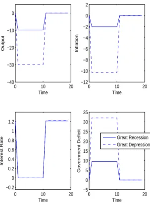
0 10 20 −40 −30 −20 −10 0 Time Output 0 10 20 −12 −10 −8 −6 −4 −2 0 2 Time Inflation 0 10 20 −0.2 0 0.2 0.4 0.6 0.8 1 1.2 Time Interest Rate 0 10 20 −5 0 5 10 15 20 25 30 35 Time Government Deficit Great Recession Great Depression
Figure 1: The Great Depression and the Great Recession in the model.
3
Austerity plans
3.1
De
fi
cits in a liquidity trap
Figure 1 shows the evolution of output, inflation and the nominal interest rate under our baseline parameterization. Recall that the parameters were chosen to replicate the "Great Depression" scenario and the "Great Recession" scenario in terms of the drop in output and inflation. The figure shows one realization of the shock, i.e. when it lasts for 10 quarters. Output and inflation drop due to the shock (panel a and b), and the nominal interest rate collapses to zero (panel c). Panel (d) is of most interest, relative to previous work, as it shows the increase in the deficit of the government due to the crisis given by
ˆ = ¯ (1 + ¯)[ˆ−]−¯ ¯[1 +−1] ˆ −¯ˆ (17)
where we have substituted out for wages in the expression in the last proposition using (9). As we see in panel (d) the deficit increases by 10 percent of GDP in the GR and 25 percent
in the GD scenario. This increase is from three sources. The last term on the right hand side represents the drop in sales due to the fact that overall output is reduced, and hence collection from sales and wage taxes is reduced as well. The second to last term reflects that smaller tax revenues are collected due to lower taxes on wage income. Finally, the
first term reflects the contribution of the interest rates to the deficit and the revaluation of the nominal debt due to changes in the price level (i.e. deflation will increase the real value of the debt).
As we see in the figure, the increase in deficit is of the same order as the deviation of output from its steady state. This is mostly because in the model wages drop more than GDP by a factor of −1 = (−1 +) hence the loss in revenues is very large. This is
a special feature of the model, and is driven to some extent by the fact that the labor market is completely flexible — hence wages fall substantially — less extreme numbers can be obtained with alternative specifications.
A natural question from the point of view of a policymaker is: How can we balance the budget? Here we illustrate three austerity plans which aim at short-run stabilization of the deficit. Thefirst is to cut government spending, the second to increase sales taxes and the third to increase labor taxes. Of these, thefirst two fail to reduce the deficit while the last one is effective. More explicitly, we now study the following policies which replace A2.
A4 (ˆˆ ˆ) = (ˆ ˆ ˆ) = 0for∀ ≥ and (ˆˆ ˆ) = (ˆ ˆ ˆ)for∀ Lump-sum taxesˆ at dates≥are set so that the government budget constraint is satisfied whileˆ= 0 for ∀
The equations the model satisfies (taking into account there existence of a unique bounded solution in the short run and the solution at ≥ using same argument as in Proposition 1) are then for any0
(1−) ˆ =−++ + (1−) ˆ−(1−)ˆ (18) =ˆ+(ˆ + ˆ −− 1ˆ) + (19) ˆ = ¯ (1+¯)[ˆ−]+[1+¯ ¯ −1] ˆ −¯[1+¯]ˆ−[1+¯ ¯ ]ˆ−[¯ +¯¯(1+−1)] ˆ (20) For preliminaries and reference, Proposition 3 and 4 show the effects government spend-ing and taxes have on output at positive and zero interest rates, while Table 2 uses the
proposition to compute tax and spending multipliers using our numerical example. The question these propositions answer is what the effect is of a unit change in each of the
fiscal instruments on output, but these statistics are discussed in more detail in Eggertsson (2010) under a slightly different policy rule. We see that government spending increases output at zero interest rates more than one to one, while sales tax cuts are also expansion-ary. Meanwhile labor tax cuts are contractionary as further discussed in Eggertsson (2010). Let us denote 4ˆ = ˆ −ˆ as the percentage change in variable ˆ due to a particular policy intervention. Thus the statistic 4ˆ
4ˆ where4ˆis an endogenous variable
measures a policy multiplier. The following propositions follows from solving (18) and (19) using this notation. The next propositions summarize the output multipliers of the policy instruments at zero and positive interest rates.
Proposition 3 Suppose A1,A3 and A4.The output multiplier of government spending at
positive and zero interest rate is:
∆ˆ ∆ˆ =−1 0 if 0 (i.e. 0) and ∆ˆ ∆ˆ = (1−)(1−)− (1−)(1−)− 1 if = 0 (i.e.
0). The multipliers of sale tax cuts are identical but scaled by a factor of −
Proposition 4 Suppose A1,A3 and A4. The output multiplier of a labor tax increase is
negative at positive interest rate andflips sign and becomes positive at zero interest rate:
∆ˆ ∆ˆ = − 0 if 0 (i.e 0) ∆ˆ ∆ˆ = (1−)(1−)− 0 if = 0 (i.e 0) Table 2 0 = 0 ∆ ∆ 0.43 0.42 2.24 1.2 ∆ ∆ -0.34 -0.31 -1.76 -0.89 ∆ ∆ -0.53 -0.49 1.15 0.17
3.2
The e
ff
ect of cutting Government Spending on De
fi
cits
We now turn to the idea of idea of cutting government spending to reduce the deficit. By expression (8a) we see that this results in
4ˆ 4ˆ = 4ˆ 4ˆ + ¯ (1 + ¯) 4[ˆ−] 4ˆ −¯¯4ˆ 4ˆ −(¯+ ¯¯)4ˆ 4ˆ
If the budget is supposed to be balanced via this "austerity" policy, this number needs to be positive.
Consider first what happens at a positive interest rate. There one can confirm that 4ˆ 4ˆ = 1 4[ˆ−] 4ˆ = (1−) −1 4ˆ 4ˆ = 0and 4ˆ 4ˆ =
−1yielding the next proposition
Proposition 5 Suppose A1, A3 and A4. At positive interest rate cutting government
spending always reduces the deficit. This reduction is given by
4ˆ 4ˆ = 1 + ¯ (1 + ¯)(1−) −1 −(¯+ ¯¯)−1 0 if 0 (i.e. 0) The proof of this proposition follows from the expression above and the fact that 0
(¯ + ¯¯)−1 = (¯ + ¯¯)−1−+1 1 and hence at a positive interest rate cutting government spending will always reduce a deficit (or create a surplus) given our specification for monetary policy. This can be seen in Table 3 for our numerical example. Observe that this statistic is close to one but can either be smaller than one or greater than one due to the fact that on the one hand a cut in government spending reduces real interest rates, and thus the interest rate burden of debt, but on the other hand it reduces output thus suppressing sales and labor tax revenues.
Table 3 0 = 0 ∆ ∆ 1.27 1.38 -1.65 -0.2 ∆ ∆ -1 -1.1 1.1 -0.1 ∆ ∆ -0.7 -0.7 -3 -1.6
Let us now consider a more interesting case when the nominal interest rate is zero. Can this overturn the result? The next proposition shows that the answer is yes at zero interest rates.
Proposition 6 Suppose A1,A3 and A4. At zero interest rate cutting government spending
can either increase or reduce the deficit at the following rate:
4ˆ 4ˆ = 1− ¯ (1 + ¯)[ (1−) (1−)(1−)−] −¯(1−)(1−)− (1−)(1−)− −¯ ¯[(1 +)(1−)(1−)− (1−)(1−)− ] if = 0
Proof. This is most easily derived by first noting that at zero interest rates by (20) 4ˆ 4ˆ =− ¯ (1 + ¯) 4 4ˆ + [1 + ¯ ¯ −1] −[¯+ ¯(1 +−1)]4ˆ
4ˆ Now use the expression for the output multiplier in (3) and note that 4
4ˆ = 1− 4ˆ 4ˆ − 1−−
1 and substitute and
solve.
Let us now interpret this. Thefirst term is the same as in the past proposition, namely 1, which means that a dollar cut in government spending will result in a reduction of the deficit by the same amount. In partial equilibrium, thus, any drop in spending reduces the deficit by that amount. The other terms, as before, come about due to general equilibrium effects but now they have much more power. A cut in government spending does not only lead to a drop in government expenditures. It will also result in a reduction in government revenues, due to the fact that it leads to a reduction in the overall level of economic activity and wages and through that, a change in the price level which may raise the real value of the outstanding nominal debt. All of these general equilibrium effects are captured in the expression above. The first term captures the increase in the real value of debt if the government cuts spending that comes about due to deflation. This term is much bigger than before. The second measures the reduction in sales tax revenues due to the drop in output. Finally, the last term measures the drop in labor tax revenues due to the fact there are now lower revenues from labor taxes.
Table 3 computes the value of the deficit multiplier for the two scenarios. As we can see the deficit increases more than one for one for the GD scenario, i.e. a one dollar cut in the spending increases the deficit by 1 dollar and 65 cents. The GR scenario is less extreme. In this case, a one dollar cut in the government spending increases the deficit by about 20 cents. The main reason for the difference is that the government spending multiplier is much bigger under the Great Depression (2.2) scenario than in the Great Recession scenario (1.2).
To clarify how the result depends on the size of the multiplier, let us make the following simplification, i) linearize around 0 government debt and ii) assume that the tax on labor is levied on profits in equal proportion. Then the expression for the deficit spending multiplier can be simplified to yield
4ˆ 4ˆ = 4ˆ 4ˆ −(¯ + ¯)4ˆ 4ˆ = 1−(¯ + ¯)4ˆ 4ˆ or 4ˆ 4ˆ 0if 4ˆ 4ˆ 1 ¯ + ¯
In words: If the multiplier of government spending is larger than 1 ¯
+¯ then the deficit will
always increase when the government cuts spending at a zero interest rate.
3.3
Sales taxes with La
ff
er-type properties
Let us now consider a sales tax increase. Here the two forces are as follows i) an increase in the tax rate will tend to increase revenues for given production and ii) increase in the rate will reduce overall production. This follows exactly the same steps as in our previous proposition so that we obtain
Proposition 7 Suppose A1,A3 and A4. At positive interest increasing sales tax always
reduces the deficit. This reduction is given by
4ˆ 4ˆ =−[1 + ¯ (1 + ¯)(1−) ] +(¯+ ¯¯)0 if i0
At zero interest rate increasing the tax rate can either increase or reduce the deficit by:
4ˆ 4 = −1 + ¯ (1 + ¯) [ (1−) (1−)(1−)−] +¯(1−)(1−)− (1−)(1−)− + ¯ ¯[(1 +)(1−)(1−)− (1−)(1−)− ] if = 0
As we can see in Table 3 the result in our numerical examples show that the contrac-tionary force is dominating in the GD case, while the two forces are close to offsetting each other in the GR case. An increase in sales taxes either expands the budget deficit or leaves it almost unchanged (but at a lower level of output). An obvious implication of this is that the effect of an "austerity measure" that involves increasing sales taxes is similar to cutting government spending. It may increase the deficit rather than reducing it. Conversely cutting sales taxes may increase tax revenues, but this is akin to being on the wrong side of the "Laffer curve".
3.4
The e
ff
ect of wage taxes increase on the de
fi
cit
We now consider the effect of increasing taxes on wages, summarizing the result in the next two propositions (but the calculation follow the same steps as in Proposition 6).
Proposition 8 Suppose A1,A3 and A4.At positive interest rate increasing wage taxes has the following effect on the deficit
4ˆ
4
=−¯+[¯+ ¯¯]
At zero interest rate this expression is given by
4ˆ 4 = −¯− ¯ (1 + ¯) 1− (1−)(1−)− −¯¯[(1−)(1−) + (1−)(1−)− ]−¯ (1−)(1−)− 0
As seen in Table 3, for both scenarios this is a large negative number, i.e. increasing labor taxes cuts down the deficit considerably. The reason for this is described in Eggertsson (2010). In the model an increase in labor taxes actually increases output in the short run, via changing deflationary expectation to inflationary ones. This is due to a number of special features discussed in Eggertsson (2010). Hence we do not wish to push this short-run property of the model too far.
4
Con
fi
dence and the long run
So far we have seen that two popular policies intended to balance the budget, namely cutting government spending or increasing sales taxes, are likely to increase the deficit rather than decreasing it at a zero nominal interest rate. Both lead to a reduction in output, as documented in Table 3, which contracts the tax base. The call for "austerity" has usually been motivated by emphasizing the importance of creating a credible long-run economic environment. The deficit, then, is often pointed to as one element that may create havoc in the future. In some respects, therefore, the results above do not undercut that basic message of "austerity", but merely suggest that the short-run effect of government spending cuts or sales tax increases may increase the budget deficit rather than decrease it, and therefore, may not be very effective in restoring "confidence," at the very least to the extent this "confidence" is tied to reducing budget deficits.
But what is "confidence" more explicitly and how is it tied to the long-run? We now explore if the standard New Keynesian model supports the popular discussion of the im-portance of "confidence" in the current crisis andfind that in certain respects the answer is a qualified "yes" — if this "confidence" is taken to mean the effect of long-run expectations
on current demand. This answer is specific to the environment of zero interest rates and this gives one rational for why confidence has been so high on the agenda following the crisis of 2008.
Here we do not model directly how deficits influence the expectation of the "long run" but address that in the next section. Instead we first want to clarify the role of long-run expectations of taxes and government spending on current demand by the using the following assumption that replaces A4.
A5 (ˆˆ ˆ) = (ˆ ˆ ˆ)6= 0 for ∀≥ andˆ = ˆ = ˆ= 0 for ∀ Current and future lump sum taxes ˆ are set so that the government budget constraint is satisfied.
Let us again classify the economy in terms of the "long run" and the "short run." In the long run, assuming A3, inflation is zero according to our policy rule, i.e. = 0. Then output is given by the following propositon using equation (6)
Proposition 9 Suppose that A1, A3 and A5. Then
ˆ =−ˆ− ˆ +− 1ˆ for ≥ (21) whereˆˆandˆ
are given by policy, so long run multipliers are given by (
∆ ∆ ∆ ∆ ∆ ∆ ) = (+−1 − −)
This proposition follows from since equation (5) only pins down the nominal interest, and thus output is determined by (6). The proposition shows that higher long-run taxes reduce long-run output. Similarly, more long-run government spending increases long-run output. The reasons here are standard: higher labor and consumption taxes reduce labor supply and thus contract output, while larger government spending increases the labor supply (by increasing marginal utility of consumption). Table 4 shows the value of long-run multipliers given in the proposition and we see that the value of these are very similar in our two numerical examples.
Table 4 0 ∆ ∆ 0.43 0.42 ∆ ∆ -0.34 -0.31 ∆ ∆ -0.53 -0.49
Let us now explore under what condition the short-run output depends on these long-run variables. Let us write the equilibrium relationships (5) and (6) for the short long-run, taking into account that = 0according to our policy rule and now allow for the possibility that ˆ
ˆ andˆ
may be non-zero. We then get
(1−) ˆ = (1−) ˆ−++ (22) +(1−) ˆ−(1−) ˆ−(1−)ˆ+(1−)ˆ (23) and (1−) =ˆ+ˆ + ˆ −− 1ˆ (24)
According to our specification for monetary policy, if the zero bound is not binding, the central bank will set the nominal interest rate so that inflation is = 0 Equation (22) then simply determines the nominal interest rate, i.e.
= −1(1−) ˆ−(1−) ˆ++ (25) +−1(1−) ˆ−−1(1−) ˆ−(1−)ˆ+
(1
−)ˆ (26) Hence if we plot up these two relationships, taking monetary policy into account, in(ˆ) space we get a horizontal AD curve that is fixed at = 0 and the equilibrium is given by point A which is the intersection of the AD curve and the AS curve in (24). Observe now that movement in the long-run variables, i.e. ( ˆˆˆ) only shift the AD curve but have no effect on the equilibrium that remains in A because the AD curve is horizontal. What is going on is that the central bank will offset any movements in these variables, hence the only effect will be to change the level of the nominal interest rate without any effect on output and prices. In this sense the level of "confidence," at least as measured by expectation about long-run variables, is completely irrelevant.5
What does matter for determining the equilibrium point A is the movements in the AS curve, i.e. movement in short term taxes and spending (
). Local to point A the model behaves exactly like the model if it had perfectlyflexible prices and then aggregate demand — or what we interpret as "confidence" — plays no role.
Consider now a shock to
This shifts the AD curve to the left. The central bank will try to accommodate this shift via cuts in interest rates — that is why the AD curve
5This stark result is special to the strong assumption that the central bank targets zero inflation and
thus replicates theflexible price allocation. Underflexible prices "demand" plays no role. More generally, for example if the central bank follows a Taylor rule, there is some short-run effect of long run expectations, but they are quantitatively small which the current specification highlights sharply.
S
ˆ
SY
AD
AS
0 A BFigure 2: A large enough shock moves the AD curve to the left.
is horizontal – however it will be unable to do so beyond the point at which the zero bound becomes binding. At this point (25) becomes binding and now output is demand determined and given by
ˆ = ˆ+ 1− ++ 1− (27) + ˆ −ˆ−ˆ+ˆ (28)
which is depicted by point B in thefigure. At this point any change in (ˆˆˆˆ )will shift the AD curve and this will be reflected in movements in output, since the central bank will not change the interest rate to offset the movements in demand — either because it is unable to or because inflation is below target (and hence it will accommodate any increase in inflation). Here the "confidence" starts playing a key role, in particular, expectations about lower future wage taxes matters or more generally higher future long-run output starts to matter. Cuts in wage tax rates increasesˆ by a factor of see (21). A lower long-run government spending will also have an effect, first by reducing ˆ by a factor of −1 (see (21)), and thus short-term demand by the same amount, but also increasing
by the price of goods today relative to the future and this price is affected by government consumption in the short runrelative to long-run consumption. Long-run sales taxes work via the same mechanism as government spending, since they enter the AS and AD equation exactly the same way except for being multiplier byIntuitively higher expected long-run sales tax increases short-term demand, since it gives people incentive to spend today rather than in the future, since consumption today is taxed at a lower rate than future consumption. To summarize, and this follows straight from manipulating the expression above:
Proposition 10 Suppose that A1, A3 and A5. Then short-run output at positive interest
rate is given by
ˆ
= 0 (29)
while output at zero interest rate is given by
ˆ = (1−) (1−)(1−)− − (1−)(1−)−1 (1−)(1−)−ˆ + (1 −)(1−) (1−)(1−)−ˆ − (1−)(1−) (1−)(1−)−ˆ the multipliers (∆ ∆ ∆ ∆ ∆ ∆
)are given by the second, third and fourth coefficients respec-tively.
The numerical values of each of these multipliers are shown in table 5. We see, for example, that an expectation of higher long-run labor tax of 1 percent will reduce output in the short run by -0.8 percent. One can think of a variety of stories which may trigger higher expected long-run wage taxes and thus contract demand in the short-run. Similarly an expectation of higher long-run sales taxes has a multiplier of 1.42, and that of government spending -1.8. We thus see that the effect of committing to lower long-run spending is almost as effective as increasing it in the short-run.
Table 5 0 = 0 ∆ ∆ 0 0 -1.8 -0.78 ∆ ∆ 0 0 1.43 0.58 ∆ ∆ 0 0 -1.69 -0.66
AD B S
S Y C ASFigure 3: At zero interest rate expectations of the long-run move aggregate demand.
5
Short-run
fi
scal crisis, debt dynamics, and con
fi
-dence
How does a deficit today change expectations about future taxes and spending? And taking these expectation effects into account, what is the net effect of short-run deficits on aggregate demand? There are no simple answers to these questions because it depends upon how the deficit will befinanced in the future. Here we show that if the budget deficits arefinanced by future increases in long-run sales taxes or reductions in long-run government spending, they are expansionary, while if they arefinanced by increases in long-run labor taxes they are contractionary. This follows directly from the last section, and what we do here is to tie the long-run expectations derived there more closely to short-run deficits.This is made explicit in Assumption 6.
A6 Fiscal policy in the short and long run is given by
) ˆ= ˆ−1+ for (30)
) ˆ = ˆ
= ˆ = 0 for
) ˆ= ¯
(1 + ¯)ˆ−1 for ≥
The key assumption is that while the distortionary taxes (or government spending on goods and services) are not the direct source of the short-run deficit (see A6ii), they will need to adjust in the long-run to bring down debt to its pre-crisis level (note that ˆ is deviation of the debt from the the steady state we linearize around).The simplest way to interpret deficits/surpluses accruing in (30) is that they come about via variations in lump-sum taxes. More generally we think of these type of fiscal shocks as coming about due to shocks that do not directly affect sales or wage taxes, or the overall size of the government, but instead somefiscal transfers that occurs via other means. A banking crisis, for example, typically puts tax payers on the hook for large amounts of money, yet this increase in debt is not driven by sharp cuts in some taxrates, or increase in government spending on good and services.
If short-run variations in ˆ in equation (30) were met by increases in long-run lump-sum taxes, then that would be the end of the story since then the model would then satisfy Ricardian equivalence. Instead, we suppose that that long-run lump-sum taxes stay at their steady state at time and thus the other taxes or spending need to adjust to balance the budget. This is made explicit in A6iii where we assume that long-run fiscal policy adjust to stabilize the debt level at its original level and that this adjustment takes place over some period of time at a rate What this means is that while the government may run up deficits in the short-run, then in the long-run debt is stabilized at whatever level it was prior to the crisis (i.e. prior to the shock hitting).
Using the budget constraint (8a) we can see that from assumption A6ii it follows that
−(1 + ¯−)¯ +1− −1 (31) = [1−−1[¯+ ¯¯]] ˆ−([ ¯−[¯+ ¯¯])ˆ −[1−[¯+ ¯¯]]ˆ for ≥(32) This equation says that in the long run, the debt interest rate payments needed to
financed by either a cut in government spending or an increase in labor or sales taxes, but the coefficient in front of each fiscal variable will in general be positive. Let us define the right hand side of (31) as the budget deficit of the government,ˆwhich is thus determined at any time ≥ by ˆ =− (1 +−) +1−ˆ −1 ≥
and, as this is a negative number, the government is running a budget surplus. How is this surplus financed? Via tax increases and spending cuts. We assume that each fiscal
instrument is adjusted in fixed proportions. Let us denote by for the share of ˆ+
financed by labor taxes, the share with sales taxes and = 1− − the share
financed by a reduction in government spending. Note that this assumption implies that the deviation of taxes and government spending from steady state will decline at the same rate as the debt, i.e. at the rate Under this assumption a full specification of long-run
fiscal policy is now given by the choice of the weights To summarize:
A7 The sequence of {} at ≥ 0 implied by A6 is financed by ˆ ˆ ˆ in the fixed proportions ≡ [1− −1[¯+ ¯¯]] ˆ ˆ = (33) ≡ −([ ¯− [¯+ ¯¯])ˆ ˆ = ≡ −[1− [¯+ ¯¯]]ˆ ˆ =
Given this policy specification we can now do the following thought experiment: What is the effect of an increase in the deficit on aggregate demand? In this thought experiment recall that the deficit is driven by a cut in lump-sum taxes, and hence it has no direct effect on current demand. The effect, then, only comes about due to the effect it has on expectations about long-run taxes and the long-run size of the government. This effect will critically depend upon how the deficit is financed, which we can, using assumption A7, write as a function how the debt is paid off, i.e. via tax or spending cuts. The next proposition summarizes this.
Proposition 11 Suppose that A1, A3, A6 and A7. Then the multiplier of deficit spending
on short-run output at positive interest rate (if
0) is given by
∆ˆ
∆ˆ
= 0 (34)
while output at zero interest rate (if
0)is given by ∆ˆ ∆ˆ = (1−)(1−) [(1−)(1−)−] (1 +−) [1−−1[¯+ ¯¯]] + (1−)(1−) [(1−)(1−)−] (1 +−) [1−[¯+ ¯¯]] − (1−)(1−) [(1−)(1−)−] (1 +−) ([ ¯−[¯+ ¯¯])
Proof: See Appendix
The first part of the proposition follows directly from equation (24) because short run output at positive interest rates does not depend on long-runfiscal policy. The second part requires a little bit of algebra and is relegated to the Appendix.
Table 6 shows the effect of one dollar of deficit on short-run demand under three different assumptions about how this long-run adjustment takes place, i.e. via increase in long-run sales taxes, a cut in the long-run size of the government, and an increase in labor taxes. Hence this experiment assumes that eitheris 1 (and == 0), = 1or= 1We use the same values for the parameters as before, but now there is one additional parameter,
which determines the speed at which debt is paid back to its original level. We assume that the half-life of debt is 5 years, hence,= 09659
The results suggest that running budget deficits is expansionary if the deficit isfinanced by a reduction in the long-run size of the government or by a increase in sales taxes. Meanwhile, the effect of budget deficits is negative on short-run demand if it will befinanced via increases in long-term labor taxes. The reason for this is exactly the same as already analyzed in the last section, here we just make more explicit the way in which debt dynamics have an impact on those long-run variables. Quantitatively, we see that these "multipliers" are considerably smaller than those that depend directly on short-run taxes and spending.
Table 6 0 = 0 ∆ ∆0 0 0 0.23 0.1 ∆ ∆0 0 0 0.14 0.06 ∆ ∆0 0 0 -0.25 -0.1
6
Conclusion
In this paper we have studied how various fiscal policies affect budget deficits on the one hand, and then how budget deficits by themselves may affect short-run demand via expectations. We have left several important aspects of this issue offthe table, and let us bring only up two of them here.
A key assumption maintained throughout the paper was that inflation in the long-run is zero. Hence there was no explicit interaction between fiscal policy today and inflation expectations over the medium or long term. An important consideration, however, is that
higher inflation tomorrow. In the face of high nominal debt, in fact, the government has an incentive to inflate. If higher deficits thus trigger expectations of higher inflation, they are expansionary at zero interest rate, since that reduces the real interest rate and thus increase demand. This is documented more explicitly in Eggertsson (2006) where those links are modelled in an infinitely repeated game between the government and the private sector. Quantitatively, Eggertsson (2006), shows that these effects can be very big. Interestingly, however, that mechanism assumes that monetary and fiscal policy are coordinated, an assumption that seems inappropriate in large monetary unions. It is difficult to imagine, for example, that large amounts of Greek debt creates quantitatively significant inflation incentives for the European Central Bank, albeit this remains a topic of further study.
Another issue we have not modeled explicitly, and is an important topic for further research, is the consequence of default by the sovereign. Recently many countries in Europe, for example, have faced very high borrowing rates due tofinancial market expectations of default. From the perspective of our model, it is important to observe that the zero bound is the relevant constraint for the instrument of the monetary authority and that typically does not include a default probability. The presence of default risk is thus not relevant by itself for the monetary authority while it is of principal importance for the budget constraint of member of the monetary union. One way to model this risk is that it is afinancing cost that does not directly affect aggregate spending akin to lump-sum taxes. While this would not directly affect the first set of results, i.e. about the effect of government spending or taxes on the margin, it would tend to increase the accumulation of debt other things constant in the crisis state. The analysis of the last section would then be relevant, i.e., the effect of this on short-term demand would depend upon expectations of how this faster increase in debt would be financed in the long-run.
7
References
Blanchard Olivier and Charles M. Kahn (1980) — "The Solution of Linear Difference Models under Rational Expectations", Econometrica 48, pp. 1305-1313.
Calvo, Guillermo. (1983) “Staggered Prices in a Utility-Maximizing Framework," Jour-nal of Monetary Economics, 12: 383-98.
Christiano, L., M. Eichenbaum, and S. Rebelo (2011): "When Is the Government Spend-ing Multiplier Large?," Journal of Political Economy, 119(1), 78, 121.
versus Old Keynesian Government Spending Multipliers,” Journal of Economic Dynamics & Control, 34, 281-295.
Correia, I, Fahri, E., Nicolini, J.P, and P. Teles, (2011) "Unconventional Fiscal Policy at the Zero Bound," mimeo.
Davig, T., and E. M. Leeper (2009): “Monetary-Fiscal Policy Interactions and Fiscal Stimulus,” National Bureau of Economic Research Working Paper No. 15133.
Denes,Matthew, and Gauti Eggertsson (2009). “A Bayesian Approach to Estimating Tax and Spending Multpliers.” StaffPaper, Federal Reserve Bank of New York.
Eggertsson, Gauti (2001), “Real Government Spending in a Liquidity Trap,” mimeo, Princeton University. Available at http://www.ny.frb.org/research/economists/eggertsson. Eggertsson, Gauti (2006). “The Deflation Bias and Committing to Being Irresponsible.” Journal of Money, Credit, and Banking 36, no. 2:283—322.
Eggertsson, G. B. (2010): "What Fiscal Policy is Effective at Zero Interest Rates?," in NBER Macroconomics Annual, Volume 25, NBER Chapters. National Bureau of Economic Research.
Eggertsson, Gauti, and Michael Woodford (2003), "The Zero Interest-Rate Bound and Optimal Monetary Policy," Brookings Papers on Economic Activity, 1, 139-211, 2003.
Eggertsson, Gauti, and Michael Woodford (2004), “Optimal Monetary and Fiscal Policy in a Liquidity Trap.” International Seminar on Microeconomics 1:75—131.
Erceg, C. and J. Linde (2010), "Is there a Fiscal Free Lunch in a Liquidity Trap," International Finance Discussion Papers, Board of Governors, Washington DC.
Leeper, E.M, N. Traum and T. Walker, "The Fiscal Multiplier Morass: A Bayesian Perspective," mimeo, Indiana University.
Mertens, K. and M. Ravn, (2010) "Fiscal Policy in an Expectation Driven Liquidity Trap," CEPR DP 7931.
Mountford, A., and H. Uhlig (2009): “What Are the Effects of Fiscal Policy Shocks?,” Journal of Applied Econometrics, 24(6), 960992.
Werning, I. (2011), "Managing a Liquidity Trap: Monetary and Fiscal Policy," Working paper, MIT.
8
Proof of propositions
Proposition 12 Suppose that A1, A3, A6 and A7. Then the multiplier of deficit spending
on short-run output at positive interest rate (if 0) is given by
∆ˆ
∆ˆ
= 0 (35)
while output at zero interest rate (if
0)is given by ∆ˆ ∆ˆ = (1−)(1−) [(1−)(1−)−] (1 +−) [1−−1[¯+ ¯¯]] + (1−)(1−) [(1−)(1−)−] (1 +−) [1−[¯+ ¯¯]] − (1−)(1−) [(1−)(1−)−] (1 +−) ([ ¯−[¯+ ¯¯])
Proof: The first part of the proof follows directly 24. The second part involves a few steps.
At date ≥ then our policy commitment A3 implies that = 0. By equation 24 then ˆ =− ˆ − ˆ + −1ˆ (36)
and hence in order to determine ˆ we need to find (ˆ
ˆ ˆ). As stated in text then according to A6 −(1+−) = [1− −1[¯+¯¯]] ˆ −([ ¯− [¯+¯¯])ˆ −[1− [¯+¯¯]]ˆ and A7 says ˆ =− (1 +−) [1−−1[¯+ ¯¯]]−1 (37) ˆ = (1 +−) ([ ¯−[¯+ ¯¯])ˆ−1 ˆ = (1 +−) [1−[¯+ ¯¯]]ˆ−1 (38)