Dynamic Load-Balancing via a Genetic Algorithm

(1)

Abstract

We produce a GA scheduling routine, which with often relatively low cost finds well-balanced schedules. Incoming tasks (of varying durations) accumulate, then are periodically scheduled, in small batches, to the available processors. Two important priorities for our scheduling work are that loads on the processors are well balanced, and that scheduling per se remains cheap in comparison to the actual productive work of the processors. We also include experimental results, exploring a variety of distributions of task durations, which show that our scheduler consistently produces well-balanced schedules, and quite often does so at relatively low cost.

1: Introduction

Researchers in Genetic Algorithms have had an ongoing interest in scheduling problems. We can cite [22] Whitley, Starkweather, and Fuquay (1989), [19] Syswerda (1991), [12] Hou, Ansari, and Ren (1994), [2] Burke, Elliman, and Weare (1995), [1] Bartling and Mühlenbein (1997), [18] Ryu, Hwang, Choi, and Cho (1997), [3] Christou and Zakarian (2000), and [17] Portmann and Vignier (2000), to name but a few. Along the way there has been an especial interest in the job shop scheduling problem. Here we might pick out [4] Davis (1985), [16] Nakano and Yamada (1991), [7] Fang, Ross, and Corne (1993), [14] Kobayashi, Ono, and Yamamura (1995), [20] Van Bael, Devogelaere, and Rijkaert (1999), [15] Miyashita (2000), and [21] Vazquez and Whitley (2000), again to name but a few. In the job shop scheduling problem, the shop has m machines. Input consists of j jobs, each consisting of m subjobs, which must run on the corresponding machines, and moreover the subjobs must be done in a certain (job dependent) order. The usual goal of job shop scheduling is to obtain a small makespan, which is the length of time needed to complete work on all the jobs, as scheduled.

In this paper we are interested in a simpler scheduling problem, and we are very much interested in pragmatics. Our scheduling problem is the kind faced by a shop

with machines that quickly mill various metal parts. An operating system for a multi-processor computer also faces this same type of problem, as does a retail store which schedules workmen to install carpets. We want our scheduling algorithm to produce good answers fast enough to be practical in real-world settings.

2: The Problem

Imagine a shop, where tasks arrive from time to time for processing. We will assume that the shop has some fixed number of processors (or machines), and that any processor can process any task. Each task has a duration, which is the number of time units needed to complete the task. If the volume of tasks that arrives exceeds the inherent throughput of the shop, then inevitably tasks will pile up in a backlog. And if the volume of tasks that arrive is below the throughput of the shop, then inevitably some processors will have idle periods. Thus the interesting case is when the volume of arriving tasks essentially equals the inherent throughput of the shop. In this case we would want to schedule tasks to processors in such as way that processors are never idle (if such is possible). One simple and direct way to approach this is (to schedule no idle time intervals to the processors and) to balance the loads scheduled on the various processors. That is, to schedule so that the time obligations placed on the various processors are as nearly equal as possible.

We continue the details of our problem scenario. We expect that continuous scheduling would be inefficient. That is, it would be wasteful to re-schedule upon the arrival of each new task. So, we will form a schedule to run for the near future, set processors to work on their assigned tasks, and in the meantime let incoming tasks accumulate. When the set of currently scheduled tasks are nearing completion (specifically, a short while before a first processor would complete all its tasks), we will pause to re-schedule. Thus we intend to schedule tasks in small-ish batches. We use the term work epoch to denote a period during which processors work to process the previously scheduled tasks, and new tasks are accumulating.

We will assume it is mandatory (or at least more efficient) that once a processor has begun actual

Dynamic Load-Balancing via a Genetic Algorithm

William A. Greene

Computer Science Department

University of New Orleans

New Orleans, LA 70148

[email protected]

504-280-6755

(2)

processing of a task, the task must run to completion on that processor (i.e., tasks are non-preemptive). When we pause to re-schedule, a partially completed task (we term it incomplete) is then required to remain on its processor under the new schedule. On the other hand, it is allowed that a scheduled task whose processing has not been begun (an unstarted task) can be re-assigned to a different processor under the new schedule. We make one exception to the preceding statement. If the start-time of a scheduled task is the same moment as when we pause to re-schedule (so, if the predecessor task of the scheduled task has just that moment completed) then we again insist that the task remain with its previously scheduled processor under the new schedule (and deem this task incomplete, too). This is reasonable, since there is likely to be a set-up cost for processing a task, for instance, if the task has to be physically moved to its processor. Incidentally, we assume the duration of a task includes any set-up or tear-down costs. Note that when a work epoch ends and we pause to re-schedule, each processor has exactly one incomplete task on it (and there may also be some unstarted tasks that were scheduled on it).

There is one remaining important issue. Tasks arrive for processing over time, and for simplicity we will assume no two tasks ever arrive at exactly the same moment. Modulo the other ground rules mentioned up to this point, we want earlier arriving tasks to be scheduled for earlier start-times. Our first priority will be to balance the loads on the processors; then, during a work epoch, processors will work on their scheduled tasks in order of the arrival times of those tasks. Although it is allowed that a task T´ gets scheduled to start on its processor P´ at a later time than a later arriving task T´´ gets scheduled to start on its processor P´´, still, it will be seen that under our problem solution, no task can get delayed indefinitely, and, roughly speaking, earlier tasks get processed before later ones.

A task’s duration is a number. In all our experiments we have used duration values (time units) that are integers in the range 5 to 95. The distribution of duration values is of course quite important to how well a scheduling regime succeeds at making efficient use of the resources (here, simply the processors). The distribution might be uniform, or normal, or bi-modal, or some other distribution. We have conducted experiments with various distributions (for half of them the average duration is 50). Our later experimental results will show that our solution scheduling regime works successfully with all our studied distributions and moreover works rather cheaply with most of them.

3: The Solution Scheduler

When we refer to scheduling the “current” set of tasks, we mean those tasks left incomplete or unstarted from the previous work epoch, plus the batch of newly arrived tasks. When we schedule the current set of tasks

to the various processors, in particular we partition those tasks (into disjoint subsets, that is, and moreover, whose union is all the current tasks). As will be seen, under the new schedule, each subset will contain exactly one incomplete task. A subset’s tasks are then assigned to that processor on which the incomplete task was running. In this way, an incomplete task stays with the processor it was running on.

To balance the loads means that, upon computing the sums of the durations of the tasks assigned to the various processors, those sums are as nearly equal as we can (reasonably) make them. Thus we are partitioning a set so as to satisfy certain constraints. Problems related to our own have been studied by researchers in the field of genetic algorithms; here we have in mind [13] Jones and Beltramo (1991), [6] Falkenauer (1995), [7] Falkenauer (1998), [10] Greene (2000), and [11] Greene (2001).

Our solution scheduler finds a good schedule by running a genetic algorithm, which is akin to ones studied in [10] Greene (2000) and [11] Greene (2001). In this paragraph we synopsize our scheduling genetic algorithm, and then in the remainder of this section we give the details of the algorithm. There is a population of individuals. An individual in the population is a partition of the current set of tasks. An individual partition has a numeric error, which gets linearly transformed to a fitness value. Individuals are selected for parenting using a standard weighted roulette wheel approach. A child is formed from two parents by greedily extracting subsets from the parents, then repairing those subsets to form a partition. A single mutation step consists of transferring a task from one subset to another. Mutation of an individual is graduated: more erroneous individuals undergo more single mutation steps.

Finally, denote by N the number of processors. In our later experiments we let N be 4, 8, and 16.

3.1: Individuals

An individual is a partition of the current set of tasks, into N subsets (N being the number of processors). An individual has an error, which is a non-negative real number.

3.2: Error and Fitness

Once the set of tasks (and their durations) are known to us, then so is the ideal subset sum of durations. Namely, we total the durations of the entirety of tasks, then divide by N, the number of processors. Each subset of tasks in a partition is assigned its own error value, namely, the (absolute) difference between its actual sum-of-durations and the ideal subset sum. For the error of a partition, we use the square root of the sum of the squares (i.e., the Euclidean vector norm) of the errors of the several subsets in the partition,

(3)

. The error and the fitness of an individual should be complementary notions: the less erroneous an individual is, the more fit we should deem it. Fitness values are obtained from error values by a linear transformation, that maps the maximum error present in the population to a minimum fitness value of 1, and maps the minimum error present in the population to a maximum fitness value which we take to be 4. This is not very different from the scaling recommendation in [9] Goldberg (1989, p 77). 3.3: Selection for Parenting

We use a standard weighted roulette wheel approach. If are the individuals in the population, with respective fitnesses , then individual gets selected with a probability equal to its relative

fitness, .

We note that the least erroneous individual in the population is therefore 4 times as likely to be chosen for parenting as is the most erroneous individual.

3.4: Crossover

Some may deem it a misuse of terminology to refer to our operator as “crossover”, since ours is markedly different from the usual crossover operators found in genetic algorithms. It is quite greedy, as well. There are two parental partitions, from which we intend to produce a child partition. Each parent partition consists of N subsets, making 2N altogether. First, from these 2N subsets we choose the N best (i.e., least erroneous) distinct ones. These N start as the subsets of the child. But these N subsets may not form a partition of the set of tasks at hand, for these N subsets may exhibit some overlapping, and their union may not include every task at hand. Repair is needed. Now we recall that, for a particular task T, we know T lies in only one subset of the first parent (since a parent’s subsets are disjoint), and likewise T lies in only one subset of the second parent. Therefore, for any particular task T, we conclude it may be present either in two child subsets (but no more than two), or one child subset, or no child subset at all. For tasks that lie in exactly one child subset, of course we make no changes. If a task lies in two child subsets, then remove it from the more erroneous child subset and leave it in the less erroneous one (flip a coin if the two subsets have equal errors).

It remains to deal with the tasks that so far appear in no child subset at all; we term these the no-show tasks. Some child subsets may not contain an incomplete task; some no-show tasks may be incomplete; the numbers of

these must be the same. So, first put each incomplete no-show task into a child subset which is lacking an incomplete task. Now round up the remaining no-show tasks, and distribute them into child subsets, by following the Most-Into-Least (MIL) heuristic: loop, inserting the no-show task of presently greatest duration into that child subset with presently the least sum-of-durations. Of course, the spirit of this heuristic is that we expect it will result in a suite of subsets whose sums are more or less equal. (And it is related to how one would pack boxes of various sizes into a container: put in the bigger boxes first and hope to fit the smaller ones around them.)

3.5: Mutation

A single mutation step consists of transferring a randomly chosen task (provided it is not an incomplete task, that is) from a randomly chosen subset to another randomly chosen subset. The mutation which an individual undergoes is graduated: the number of single mutation steps attempted is directly proportional to the individual’s relative error, with the most erroneous individual undergoing some maximum number (which we chose to be 10) of attempts at a single mutation step. And mutation of an individual is stochastic, as well: some number of attempts (as just described) are made at a single mutation step, but there is only a 50-50 chance that the attempt will continue on to the performance of a single mutation step. The most erroneous individual may undergo as many as 10 single mutation steps, and we expect it to undergo about 5.

3.6: Generational Change

In our approach, the population undergoes generational changes. The next generation of the population has the same size as the current one. To form the next one, we first practice elitism: a certain number of individuals automatically survive into the next generation. Then to fill the next generation up to size, we loop, selecting pairs of parents, and inserting their child into the next generation. Once the next generation is filled to size, we subject its members to graduated stochastic mutation, as described above, except that the elite survivors are excused from mutation. In this way, the next generation always contains some individuals that are at least as desirable as the best found in the current generation. 3.7: Stopping Conditions

We want the cost of scheduling per se to remain modest, as compared to the work done by processors while they process tasks. We are willing to accept a somewhat sub-optimal schedule, provided it can be found quickly. So, we do not allow our genetic algorithm to run very long. There are two conditions under which we stop evolving the population. We stop if the generation error partition( ) error subset( _i)2

i=1 N

∑

= a₁, , ,a₂ … a_m f₁, , ,f₂ … f_m a_j f_j⁄(Σ_if_i)

(4)

number reaches the same as the number of processors, N. Also we stop if there appears an individual (partition) that is good enough. We let the latter mean, if the partition’s error is no more than . That number is the error of a partition whose every subset has error equal to 1.0. Since in our experiments, task durations commonly average 50 time units, and there are multiple tasks assigned to each processor, an error of one time unit in each processor means the loads have been balanced to a rather high degree.

What may surprise the reader is how successful the algorithm is at finding near perfectly balanced schedules after just a few generations.

Of course, once we stop evolving the population, the schedule returned by our scheduling module is the best individual ever found (which will be the best individual in the last generation).

3.8: Summary

We trust our program now is clear. During a work epoch, processors work on tasks that have been assigned to them. Just a bit before some first processor would complete all tasks scheduled for it, we pause to re-schedule. Incomplete and unstarted tasks from the previous schedule, plus tasks that have accumulated during the work epoch, are the ones assigned in the new schedule. We want scheduling per se to have low cost. And we want schedules to exhibit load balancing. If loads are poorly balanced by the scheduler, the next pause to re-schedule will come too quickly, before very many tasks have completed, making our shop churn around scheduling.

Here are the last programmatic details. We kept population size quite small, just 20 individuals for all experiments. The number of elite survivors across a generational change is 2. We end a work epoch and pause to re-schedule when a mere 2 time units remain before some first processor would complete all its tasks.

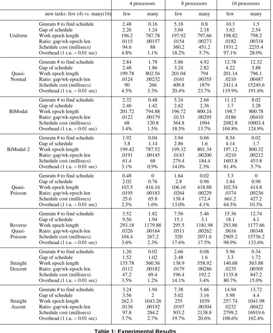
4: Experimental Results

We report on 48 experiments. There are three variables that differentiate between our experiments. One is the number N of processors; we let N have three different values: 4, 8, and 16. The second variable is how many tasks need to be scheduled. We chose two alternatives, few (meaning on average 4 per processor) versus many (on average 16 per processor). For the “few” alternative, we make 4 * N new tasks accumulate during a work epoch, and for the “many” alternative we make 16 * N accumulate.

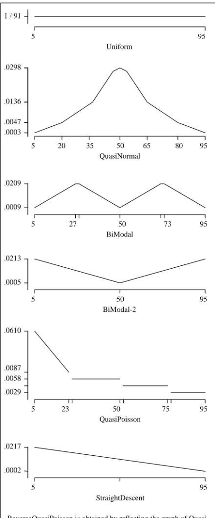
The third variable is the distribution of the durations of the tasks. We studied eight distributions: uniform, quasi-normal, two bi-modal ones, a quasi-Poisson

distribution and its mirror image, plus two more that we have termed straight descent and straight ascent. All the_{probability distribution functions we used are piecewise} N 1 / 91 5 95 Uniform .0213 .0005 5 50 95 BiModal-2 .0136 .0047 .0003 .0298 5 20 35 50 65 80 95 QuasiNormal .0209 .0009 5 27 50 73 95 BiModal .0610 .0029 5 23 50 75 95 QuasiPoisson .0058 .0087 .0217 .0002 5 95 StraightDescent

ReverseQuasiPoisson is obtained by reflecting the graph of Quasi-Poisson across the vertical line x = 50. Similarly is StraightAscent obtained from StraightDescent.

(5)

linear mappings; their graphs are given (sometimes in exaggerated form) in Figure 1; their exact mathematical definitions are given in an appendix. For all eight

distributions, the duration values fall in the range from 5 to 95 time units. For the first four distributions the average duration is 50 time units. For these four

4 processors 8 processors 16 processors

new tasks: few (4) vs. many(16) few many few many few many

Genratn # to find schedule 2.48 0.16 5.18 0.8 10.3 1.5

Gap of schedule 2.26 1.24 3.04 2.18 3.62 2.54

Uniform Work epoch length 196.2 787.78 197.92 797.66 198.82 798.2

Ratio: gap/wk-epoch-len .0115 .00157 .0154 .00273 .0182 .00318

Schedule cost (millisecs) 94.6 88 360.2 451.2 1931.2 2235.4

Overhead (1 t.u. = 0.01 sec) 4.8% 1.1% 18.2% 5.7% 97.1% 28.0%

Gap of schedule 2.48 1.86 3.24 2.82 4.22 3.88

Quasi- Work epoch length 199.78 802.56 201.04 794 201.14 796.1

Normal Ratio: gap/wk-epoch-len .0124 .00232 .0161 .00355 .0210 .00487

Schedule cost (millisecs) 90 266 409.8 1879 2411.4 15249.6

Overhead (1 t.u. = 0.01 sec) 4.5% 3.3% 20.4% 23.7% 119.9% 191.6%

Gap of schedule 2.46 1.42 2.62 2.36 3.7 3.28

BiModal Work epoch length 201.72 794.88 196.72 800.24 198.7 800.78

Schedule cost (millisecs) 68 120.8 364.8 1094 2082.8 10003.4

Overhead (1 t.u. = 0.01 sec) 3.4% 1.5% 18.5% 13.7% 104.8% 124.9%

Gap of schedule 3.8 1.14 2.86 1.6 4.14 1.7

BiModal-2 Work epoch length 199.42 787.52 199.32 801.34 197.12 800.32

Schedule cost (millisecs) 61.4 68 279.4 184.4 1603.8 453.8

Overhead (1 t.u. = 0.01 sec) 3.1% 0.9% 14.0% 2.3% 81.4% 5.7%

Genratn # to find schedule 0.48 0 1.64 0.02 3.3 0

Gap of schedule 2.02 0.76 2.8 0.96 3.84 0.98

Quasi- Work epoch length 103.5 416.16 106.16 418.88 102.54 414.8

Poisson Ratio: gap/wk-epoch-len .0195 .00183 .0264 .00229 .0374 .00236

Schedule cost (millisecs) 25.6 65.8 138.4 172.4 661.2 427.2

Overhead (1 t.u. = 0.01 sec) 2.5% 1.6% 13.0% 4.1% 64.5% 10.3%

Gap of schedule 9.56 1.94 15.1 3.1 18.1 4.1

Reverse Work epoch length 293.18 1179.88 295.5 1181.98 293.86 1177.66

Quasi- Ratio: gap/wk-epoch-len .0326 .00164 .0511 .00262 .0616 .00348

Poisson Schedule cost (millisecs) 104.4 267.2 520 2071.6 2905.2 15736.2

Overhead (1 t.u. = 0.01 sec) 3.6% 2.3% 17.6% 17.5% 98.9% 133.6%

Gap of schedule 1.52 1.02 2.48 1.6 3.3 1.72

Straight Work epoch length 135.78 560.56 138.9 558.92 140.68 563.88

Descent Ratio: gap/wk-epoch-len .0112 .00182 .0179 .00286 .0235 .00305

Overhead (1 t.u. = 0.01 sec) 3.5% 1.2% 14.1% 3.4% 80.7% 15.0%

Gap of schedule 3.56 2 5.02 3.16 5.98 4.4

Straight Work epoch length 262.3 1043.26 255 1039 257.74 1041.98

Ascent Ratio: gap/wk-epoch-len .0136 .00192 .0197 .00304 .0232 .00422

Overhead (1 t.u. = 0.01 sec) 3.7% 2.7% 19.7% 20.6% 108.6% 162.4%

(6)

distributions, we can now make two predictions: when few (meaning 4) new tasks (per processor) accumulate, we expect the work epochs to run for approximately 4 * 50 = 200 time units, and when many (16) new tasks accumulate, we expect the work epochs to run for approximately 800 time units.

How will we measure the worthiness of our scheduler? We will look at two measurements. The first is a ratio. Each subset of tasks in a schedule has its own sum of durations. Define the gap of a schedule to be the difference between the greatest and least such sum. The smaller is the gap of a schedule, the more nearly balanced are the loads on the processors under the schedule. Also, each work epoch runs for some number of time units which of course depends upon when a first processor would complete all its tasks. On a trial of our scheduler, we will have it schedule for 50 successive work epochs. Our first measurement of scheduling success will be the ratio of average gap over average work epoch length, over the 50 successive work epochs. This ratio rewards load balancing in two ways. The better balanced are the loads, the smaller is the numerator in this ratio. And, the better balanced are the loads, the longer till we must pause to re-schedule, so the greater is the denominator in this ratio. So, a smaller ratio indicates greater success at balancing loads.

Our second measurement of the efficiency of our scheduler will be more concrete and topical. We will record the average actual time, measured in milliseconds, that scheduling takes, when we run our software on some particular CPU, in our case, a 200 Mhz Pentium II.

Table 1 shows the experimental results. 4.1: Analysis of Results

The scheduler devises excellent schedules, often at surprisingly low cost, over all the distributions studied.

The eight major horizontal blocks in Table 1 correspond to the eight distributions of task durations. Examining line number 1 in each block, the reader may be surprised at how few generations (of merely 20 individuals) are needed before the genetic algorithm finds an acceptable schedule. We feel this is mostly attributable to how well the greedy crossover operator succeeds in manufacturing good (well-balanced) offspring. Examining line number 2 in each block shows consistently small gaps, except for the cases when there are few (4) tasks accumulating from the reverse-quasi-Poisson distribution. Examining line number 3 in each block of the first 4 distributions, we discover the work epoch lengths (approximately 200 or 800) which were predicted a few paragraphs earlier. Examining line number 4 in each block, the ratio of gap to work epoch length is low; it averages 0.022 when there are few (4) new tasks accumulating and averages 0.0027 when many (16) new tasks are accumulating. We conclude that schedules exhibit excellent load balancing. Examining

line number 5 in each block, the actual run times vary. Generally, actual measured run times are lowest when there are 4 processors and few new tasks accumulating, and the times are highest when there are 16 processors and many new tasks accumulating.

Line number 6 in each block, for overhead, has not yet been described. It addresses the issue of which shop scenarios are ones in which our scheduler would be practical. We want the cost of scheduling to be low, in comparison to the time our N processors spend doing their intended productive work. To get a feel for when this is so, we equate 1 time unit to one-hundredth of a second (then, for the first four distributions, average task duration of 50 time units equates to half a second). Finally, line number 6 shows the ratio of line number 5 (actual measured scheduling time, in milliseconds) over the time from line number 3 (work epoch length) adjusted to milliseconds. The reader will see that often these ratios are quite low. For instance, when there are 4 processors, the overhead is just several percentage points. When there are 16 processors, the overhead frequently appears to be very high. But this does not mean our genetic approach to scheduling is untenable; instead it means it will be practical only if a time unit is greater that one-hundredth of a second, such as perhaps one-tenth of a second as opposed to one-hundredth of a second. Also, where the shown overhead appears too high for practicality, one can consider using a faster CPU than ours for running the scheduler. As of this writing, CPU’s that are five times faster than ours are widely available for PC’s.

Here are some other observations that occur to us. Let us compare the columns for “many” new tasks, to the columns for “few” new tasks. Invariably, having many (16) new tasks per processor to schedule, compared to having few (4), results in a better schedule per se (though also usually taking longer to concoct). Indeed, when there are many new tasks per processor to schedule, we see that fewer generations are needed to find an acceptable schedule, and gaps are smaller as well, leading to markedly lower ratios (lines 4). This can probably be explained by reasoning that more tasks to work with gives the scheduler greater leeway to find a balanced load.

Our scheduler worked best on the quasi-Poisson distribution, and nearly as well on the somewhat similar straight-descent distribution. (Also the bi-modal-2 distribution was comparably easy.) The explanation would appear to be that having just a few lengthy tasks but many short tasks allows the scheduler, using the MIL (most into least) heuristic, to quickly find well-balanced loads. Indeed, sometimes it found an acceptable schedule already in generation zero! This can be explained by how the populations were initialized. Individuals in the initial population were manufactured by assigning certain portions (such as 25%) of the tasks at random to the N subsets, then assigning the remaining tasks to subsets by using the MIL heuristic. We surmise that the MIL heuristic is a very good one.

(7)

Complementarily, the scheduler was most challenged by the reverse-quasi-Poisson distribution, and its relative, straight-ascent. Here the picture is reversed: substantial numbers of lengthy tasks but few short tasks make it hard to find a balanced schedule.

We were surprised that the quasi-normal distribution was as troublesome as it was. It was more troublesome, for instance, than either of the bi-modal distributions.

Finally, let us observe that the processors need not be put into suspension while the scheduler runs. If we assume we are in a scenario where it is practical to use our scheduler, then the scheduler does not take very long to run and can be started up in time for it to complete before some first processor would complete all its tasks. Or, approaching the issue a little differently, we can view the next episode of scheduling as just another incoming task, that arrives late in the batch.

5: Conclusions

We have developed a scheduling routine, based upon a genetic algorithm, which is very effective and which, in many cases, has relatively low cost. It is usable in real-world settings in which tasks of varying durations arrive and need to be scheduled to a set of available processors. A principal goal of the scheduler is that it produce schedules that to a high degree balance the loads placed on the various processors. Another goal is that scheduling itself should have an affordable cost, when compared to the work done as processors process the incoming tasks.

We have run 48 scheduling experiments, incorporating 8 different task distributions. In all experiments the scheduler produced well-balanced schedules. In many cases the time-cost of scheduling per se was quite affordable; frequently it was just a few percentage points of the time spent by the processors. A surprising quality of the scheduler is how successful it is at finding near perfectly balanced schedules in just a few generations.

Appendix

In this appendix we provide the exact mathematical definitions for our distribution functions.

A nonnegative-valued function is normalized if the sum of its values equals 1.0. A probability distribution function is a normalized, nonnegative-valued function. Below are given the definitions of non-normalized versions of functions. The suggestive graphs in Figure 1 refer to values of their normalizations.

QuasiNormal: y = , for x in [5, 19]; , for x in [20, 34]; , for x in [35, 49]; 53.5, for x = 50; , for x in [51, 65]; , for x in [66, 80]; , for x in [81, 95]. BiModal: y = , for x in [5, 27]; , for x in [28, 50]; , for x in [51, 72]; , for x in [73, 95]. BiModal-2: y = , for x in [5, 50]; , for x in [51, 95]. QuasiPoisson: y = , for x in [5, 23]; 2, for x in [24, 55]; 1.5, for x in [56, 80]; 1, for x in [81, 95]. StraightDescent: y = , for x in [5, 95].

The ReverseQuasiPoisson distribution is obtained by reflecting the QuasiPoisson distribution across the vertical line x = 50. Similarly, StraightAscent is obtained by reflecting StraightDescent across that vertical line. References

1. U. Bartling and H. Mühlenbein (1997). Optimization of large scale parcel distribution systems by the Breeder Genetic Algorithm (BGA). In T. Bäck (ed.), Proceedings of the

Seventh International Conference on Genetic Algorithms,

pp 473-480. Morgan Kaufmann Publ., San Francisco, CA.

2. E. K. Burke, D. G. Elliman, and R. F. Weare (1995). A hybrid genetic algorithm for highly constrained timetabling problems. In L. J. Eshelman (ed.) Proceedings of the

Sixth International Conference on Genetic Algorithms, pp

605-610. Morgan Kaufmann Publ., San Francisco, CA. 3. T. Christou and A. Zakarian (2000). Domain knowledge and

representation in genetic algorithms for real world scheduling problems. In D. Whitley et al. (eds.),

Proceedings of the 2000 Genetic and Evolutionary Computation Conference, pp 690-696. Morgan

Kaufmann Publ., San Francisco, CA.

4. L. Davis (1985). Job shop scheduling with genetic algorithms. In J. Grefenstette (ed.), Proceedings of an International

Conference on Genetic Algorithms and their

Applications, pp 136-140. Lawrence Erlbaum, Hillsdale,

NJ.

5. E. Falkenauer (1995). Solving equal piles with the Grouping Genetic Algorithm. In L. J. Eshelman (ed.), Proceedings

of the Sixth International Conference on Genetic

1 2 --- x–2 x–11.5 2x–45.5 2x – +154.5 x – +88.5 1 2 --- x – +48 x–4 x – +51 x–49 x – +96 x – +51 x–49 x – +26 x – +96

(8)

Algorithms, pp 492-497. Morgan Kaufmann Publ., San

Francisco, CA.

6. E. Falkenauer (1998). Genetic Algorithms and Grouping

Problems. John Wiley & Son, New York, NY.

7. H.-L. Fang, P. Ross, and D. Corne. (1993). A promising genetic algorithm approach to job-shop scheduling, re-scheduling, and open-shop scheduling problems, In S. Forrest (ed.), Proceedings of the Fifth International

Conference on Genetic Algorithms, pp 375-382. Morgan

Kaufmann Publ., San Mateo, CA.

8. T. C. Fogarty, F. Vavak, and P. Cheng (1995). Use of the genetic algorithm for load balancing of sugar beet presses. In L. J. Eshelman (ed.) Proceedings of the Sixth

International Conference on Genetic Algorithms, pp

617-624. Morgan Kaufmann Publ., San Francisco, CA. 9. D. Goldberg (1989). Genetic Algorithms in Search,

Optimization, and Machine Learning. Addison-Wesley,

Reading, MA.

10. W. A. Greene (2000). Partitioning sets with genetic algorithms. In J. Etheredge and B. Manaris (eds.),

Proceedings of the Thirteenth International Florida Artificial Intelligence Research Society Conference

(FLAIRS-2000), pp 102-106. AAAI Press, Menlo Park, CA.

11. W. A. Greene (2001). Genetic algorithms for partitioning sets. International Journal on Artificial Intelligence Tools 10(1/2), pp 225-241. World Scientific Publ., River Edge, NJ.

12. E. Hou, N. Ansari, and H. Ren (1994). A genetic algorithm for multiprocessor scheduling. IEEE Transactions on

Parallel and Distributed Systems 5(2), pp 113-120.

13. D. R. Jones and M. A. Beltramo (1991). Solving partitioning problems with genetic algorithms. In K. R. Belew and L. B. Booker (eds.), Proceedings of the Fourth International

14. S. Kobayashi, I. Ono, M. Yamamura (1995). An efficient genetic algorithm for job shop scheduling problems. In L. J. Eshelman (ed.) Proceedings of the Sixth International

15. K. Miyashita (2000). Job-shop scheduling with genetic programming. In D. Whitley et al. (eds.), Proceedings of

the 2000 Genetic and Evolutionary Computation Conference, pp 505-512. Morgan Kaufmann Publ., San

Francisco, CA.

16. Nakano and T. Yamada (1991). Conventional genetic algorithms for job-shop problems. In R. Belew and L. Booker (eds.), Proceedings of the Fourth International

Kaufmann Publ., San Mateo, CA.

17. M.-C. Portmann and A. Vignier (2000). Performances study on crossover operators keeping good schemata for some scheduling problems. In D. Whitley et al. (eds.),

Proceedings of the 2000 Genetic and Evolutionary Computation Conference, pp 331-338. Morgan

18. R. Ryu, J. Hwang, H. R. Choi, and K. K. Cho (1997). A genetic algorithm hybrid for hierarchical reactive scheduling. In T. Bäck (ed.), Proceedings of the Seventh

International Conference on Genetic Algorithms, pp

497-504. Morgan Kaufmann Publ., San Francisco, CA. 19. G. Syswerda (1991). Schedule optimization using genetic

algorithms. In L. Davis (ed.) Handbook of Genetic

Algorithms, pp 332-349. Van Nostrand Reinhold, New

York, NY.

20. P. Van Bael, D. Devogelaere, and M. Rijckaert (1999). The job shop problem solved with simple, basic evolutionary search elements. In W. Banzhaf et al. (eds.), Proceedings

of the 1999 Genetic and Evolutionary Computation Conference, pp 665-669. Morgan Kaufmann Publ., San

Francisco, CA.

21. M. Vazquez and D. Whitley (2000). A comparison of genetic algorithms for the dynamic job shop scheduling problem. In D. Whitley et al. (eds.), Proceedings of the

2000 Genetic and Evolutionary Computation Conference,

pp 1011-1018. Morgan Kaufmann Publ., San Francisco, CA.

22. D. Whitley, T. Starkweather, and D. Fuquay (1989). Scheduling problems and traveling salesman: the genetic edge recombination operator. In D. Schaffer (ed.),

Proceedings of the Third International Conference on Genetic Algorithms, pp 133-140. Morgan Kaufmann