Defaultable Security
Valuation and Model
Research Paper N° 28
FAME - International Center for Financial Asset Management and Engineering 40, Bd. du Pont d’Arve PO Box, 1211 Geneva 4 Switzerland Tel (++4122) 312 09 61 Fax (++4122) 312 10 26 http: //www.fame.ch E-mail: [email protected] March 2001
Risk
Aydin AKGUNINTERNATIONAL CENTER FOR FINANCIAL ASSET MANAGEMENT AND ENGINEERING
• • • •
R
ESEARCH
P
APER
S
ERIES
The International Center for Financial Asset Management and Engineering (FAME) is a private foundation created in 1996 at the initiative of 21 leading partners of the finance and technology community together with three Universities of the Lake Geneva Region (Universities of Geneva, University of Lausanne and the Graduate Institute of International Studies).
Fame is about research, doctoral training, and executive education with “interfacing” activities such as the FAME lectures, the Research Day/Annual Meeting, and the Research Paper Series.
The FAME Research Paper Series includes three types of contributions:
• First, it reports on the research carried out at FAME by students and research fellows. • Second, it includes research work contributed by Swiss academics and practitioners
interested in a wider dissemination of their ideas, in practitioners' circles in particular. • Finally, prominent international contributions of particular interest to our constituency are
included as well on a regular basis.
FAME will strive to promote the research work in finance carried out in the three partner Universities. These papers are distributed with a ‘double’ identification: the FAME logo and the logo of the corresponding partner institution. With this policy, we want to underline the vital lifeline existing between FAME and the Universities, while simultaneously fostering a wider recognition of the strength of the academic community supporting FAME and enriching the Lemanic region.
Each contribution is preceded by an Executive Summary of two to three pages explaining in non-technical terms the question asked, discussing its relevance and outlining the answer provided. We hope the series will be followed attentively by all academics and practitioners interested in the fields covered by our name.
I am delighted to serve as coordinator of the FAME Research Paper Series. Please contact me if you are interested in submitting a paper or for all suggestions concerning this matter. Sincerely,
Prof. Martin Hoesli
University of Geneva, HEC 40 bd du Pont d'Arve 1211 Genève 4
Tel: +41 (022) 705 8122 [email protected]
Defaultable Security Valuation and Model Risk
Aydin Akgun
1,2This Version: March 2001
1HEC, University of Lausanne, and FAME (International Center for Financial Asset
Management and Engineering), Geneva, Switzerland. I would like to thank my thesis su-pervisor Prof. Rajna Gibson (ISB, University of Zurich) for her continual support through-out the study. The financial support of RiskLab (Zurich) is gratefully acknowledged. All comments are welcome.
2Address:Swiss Banking Institute, University of Zurich, Plattenstrasse 14, 8032 Zurich,
Abstract
The aim of the paper is to analyse the effects of different model specifications, within a general nested framework, on the valuation of defaultable bonds, and some credit derivatives. Assuming that the primitive variables such as the risk-free short rate, and the credit spread are affine functions of a set of state variables following jump-diffusion processes, efficient numerical solutions for the prices of several defaultable securities are provided. The framework is flexible enough to permit some degree of freedom in specifying the interrelation among the primitive variables. It also allows a richer economic interpretation for the default process. The model is calibrated, and a sensitivity analysis is conducted with respect to parameters defining jump terms, and correlation. The effectiveness of dynamic hedging strategies are analysed as well.
1
Introduction
The aim of this paper is to analyse model risk within the context of credit risk mod-eling, and more specifically for defaultable bonds and credit derivatives. With the proliferation of financial losses related to the use of derivative securities risk man-agement in general, and model risk manman-agement in particular has gained attention in the recent years. Recently, the booming credit risk literature has experienced a shift towards the so called reduced-form models that rely, basically, on an exogenous specification of default-inducing processes. The reason is that these models are more amenable to empirical testing and, given suitable assumptions on recovery rates, al-low straightforward application of the already available martingale pricing technology. In this vein, it is also easier to analyse market risk and credit risk together, which is crucial for versatile financial institutions operating in dynamic and intertwined environments.
The paper contributes to the credit risk literature in several ways. First, de-faultable securities are priced in a framework that is unprecedented in its generality. Second, an extensive analysis of the effects, on valuation, of jump terms in both riskless interest rates and credit spreads is provided. Third, the influence of corre-lation between riskless interest rates and credit spreads is also analysed both from valuation, and hedging perspectives. Although jumps in interest rates recently have received some attention (see Akgun (2000) and references therein), the presence of jumps in credit spread dynamics has been so far ignored in both the empirical and theoretical literature.1 As the distributions implied by observed credit spread dy-namics are highly leptokurtic the relevance of incorporating jumps into the analysis becomes clear. There has also been a relatively higher but mostly qualitative interest in the correlation between market and credit risks, especially from a risk measure-ment perspective. The analysis in this paper, specifically sets out to quantify the effects of this correlation in pricing and hedging several defaultable securities. The framework of the paper is basically as follows. There are three state variables follow-ing jump-diffusion processes. The diffusion part is of CIR (1985) type. The riskless short-rate and the credit spread are affine functions of the state variables. There are three types of jumps. Jumps unique to the interest rate, jumps pertaining to the credit spread, and jumps common to both processes with a joint jump-size distribu-tion depending only on time. The diffusion part formulation is such that negative correlation between credit spreads and interest rates is allowed, and positivity of the spread is guaranteed. The positivity is no longer guaranteed when one takes into account the normally distributed jump sizes. Empirically, however, it turns out that negative state variables are possible only with a very small probability. The model also is admissible in the sense of Dai and Singleton (1999). Volatilities, drifts, and intensities can be stochastic provided they are affine in state variables. Such a frame-work permits one to distinguish the effects of economy-wide shocks fromfirm-specific 1The empirical evidence for jumps in the dynamics of credit spreads is not lacking. LTCM is believed to have lost more than $500 million because of a jump of nearly %17 in credit spreads. Such jumps become especially important when the correlation structure of state variables defining interest rate and credit risks is substantially altered duringfinancial market turmoil.
ones, as well as being open to other interpretations for the jump terms. More impor-tantly, one can see the effects of the interaction between market risk and credit risk. Tractable solutions of this model are possible using the affine-pricing methodology developed by Duffie, Pan, and Singleton (1999), and Bakshi and Madan (1999) which involves decomposing an option-like payoffinto principal securities, and valuing each of these through the Fourier inversion of its characteristic function. Model parameters can be estimated in two steps as in Duffee (1999) if one assumes away the common jump term. This is essential for estimation since simultaneous use of the treasury bond data and corporate bond data to estimate the whole set of parameters would be cumbersome and highly impecise.
Given this setup, the aim is to analyse the effects, on pricing, of different specifi-cations regarding the jump terms and the correlation between the riskless short-rate and the credit spread. The securities that will be priced, as examples, are a de-faultable bond, a put option on the dede-faultable bond, a credit spread option, and a call option on the credit spread. Analysing these credit derivatives with different payoff structures will allow a better assessment of the relation between market risk and credit risk, and differential impact of jump terms. In this regard, conducting sensitivity analysis with respect to relevant parameters may provide further insights. The efficiency of modelisation can also be tested in this nested framework, in terms of pricing. It is at this point that an analysis from the perspective of model misspeci-fication becomes relevant. Aside from pricing issues, improvements gained with more realistic assumptions in the partial hedging of defaultable securities can be compared to those of simpler models. Before closing this section, note that any attempt to quantify model risk is dependent on a chosen benchmark model. The benchmark model is implicitly assumed to be closer to reality, and the performance, in an ap-propriately defined sense, of any submodel that is inferior to it can be evaluated and quantified with respect to the benchmark model. Such an analysis is especially of importance from the viewpoint of an economic agent trying to select or evaluate a model to use in pricing, trading, or hedging derivative securities.
Before explaining the theoretical framework it may be illustrative to briefly touch upon the related literature which would also allow a better comparison with the present article. There are two, quite distinct, brands of research focusing on the pricing of credit risk. These are named as structural, and reduced-form approaches. The structural approach represents and encompasses various extensions of Merton (1974)’s work on the pricing of corporate debt. In this brand of the literature default occurs when the firm asset value process hits a lower boundary that can be prede-termined andfixed (for instance the face value of debt) or endogeneously determined as the outcome of bargaining between shareholders and creditors. The problem with such models is that to be realistic they need to specify, rather elaborately, the condi-tions triggering default and the capital structure of thefirm in question. Even with a complex specification, however, the empirical performance of these models have been disappointing. Moreover, by their very nature (since default stopping time is not in-accessible), they sharply underestimate credit spreads for short time horizons. These and other considerations led researchers to model the default event exogeneously, as the first jump of a Cox process with certain intensity for instance. Jarrow and
Turnbull (1995) article is one of the precursors in this area. In their model default time is exponentially distributed, with constant intensity and the default process is independent of the riskless interest rate. Their approach involves building trees for the riskless term structure and the default process, and inferring risk-neutral default probabilities from the observed market prices of corporate bonds. This model has been later extended to the case where default time follows a continuous-time discrete state Markov chain to allow valuation of derivatives based on credit ratings. (See Jar-row, Turnbull, and Lando (1997), and Lando (1998). There has also been attempts to recast the HJM (1992) framework to take into account default risk by modeling de-faultable forward rates directly and then derive the restrictions necessary to rule out arbitrage. Das and Tufano (1995), and Schönbucher (1998) can be cited as examples. Yet another subgroup of research within reduced-form models have been initiated by Duffie and Singleton (1999). Assuming that recovery value, upon default, is propor-tional to the market value an instant before default they showed that the ordinary martingale valuation methodology can still be used to value defaultable bonds by adding an adjustment term to the riskless discount rate. The present paper departs from these and other previous research in several ways. First, it represents the first attempt to model credit spreads as jump-diffusions. Second, as explained above the proposed model is very general in other aspects as well. Third, in the empirical part accompanying the theoretical pricing framework an extensive sensitivity analysis is conducted from a model risk perspective.
The paper proceeds as follows: First, the reduced form approach is outlined briefly. In the next section the theoretical framework is laid out in its full generality, and transform analysis, and credit derivative valuation are explained. Section 3 deals with the particular model proposed along with subsections on data and implementation issues, hedging considerations, and the details of the numerical integration techniques employed. In Section 4 results are presented and interpreted from a model risk perspective. Section 5 concludes with a discussion assessing the relevance of the findings for pricing credit sensitive securities, and for risk management.
1.1
The Reduced Form Approach
In this subsection, we briefly present the valuation formula resulting from the work of Duffie and Singleton (1999). This formula will be the essential pricing ingredient for a large part of this paper. Assume that markets are perfect and an equivalent martingale measure exists. Consider a defaultable claim with a random promised payoff ofH at maturity T. When default occurs at time Td, it is unpredictable, and it involves a loss rate of L(Td) in the market value of the claim. Hence, the value at time t of this claim can be written, under the risk neutral measure, as
St=Et exp − TZΛTd t rsds hHI {T <Td }+S(Td) ¡ 1−L(Td)¢I {T≥Td } i (1)
St=Et exp − T Z t Rsds H (2)
with Rt = rt+htLt where ht denotes the hazard rate of the default process. (2) means that we can value a defaultable claim as if its payoff is riskless, but discounted at a default-adjusted discount rate, given above by Rt. In this paper we are going to denote default adjustment term htLt by st and call it somewhat informally as the credit spread. Note that the same approach can be used to value coupon bonds as well. Apart from allowing straightforward discounting of payoffs of defaultable claims, the proportional loss in market value assumption helps preserve the simple value additivity rule for coupon bonds. (Jarrow and Turnbull (2000))
2
The Theoretical Framework
We operate in the context of a perfect continuous-time economy with a trading in-terval [0, T∗], T∗ being kept fixed. Uncertainty in capital markets is characterised through a probability space (Ω,=,z, P), with z = {=(t) :t∈[0, T∗]} denoting the
P−completed, right-continuousfiltration generated by a set of state variables follow-ing jump-diffusion processes. r is the instantaneous riskless interest rate which is equivalently called as the riskless short rate in this paper. The price at time t of a riskless zero-coupon (defaultable) bond maturing atT (for0< T ≤T∗)is denoted by
B(t, T)(Bd(t, T)).The existence of an equivalent martingale measure is assumed, and in the following all expectations are taken with respect to this measure unless noted otherwise.3 The state variables in the economy are denoted by an n-dimensional strong Markov process uniquely solving the followingSDE :
Xt=X0+ t Z 0 µ(Xs, s)ds+ t Z 0 σ(Xs, s)dW(s) + t Z 0 J(s)dN(s) (3)
where W is a d-dimensional independent standard Brownian motion, N is a vector Poisson process of intensity λ(Xt, t), with a random jump-size matrix J(t) whose distribution depends only on time t, and µ and σ are conformable coefficients that are affine in the state variables. For additional technical details see Duffie, Pan, and Singleton (1999). The risk-free short rate, and credit spread are also assumed to be affine in the state variables. That is,
2An important condition is that jumps in the conditional distribution ofS, h, or L occur with probability zero at the default timeTd.
3The particular choice of the equivalent martingale measure is implicitly left to the market, or to the representative agent, if any. This wave-offis typical in this brand of asset pricing literature.
µ(x, t) = µ0(t) +µ1(t)·x (4)
σ(x, t)σT(x, t) = σ0(t) +σ1(t)·x (5)
λ(x, t) = λ0(t) +λ1(t)·x (6) r(x, t) = r0(t) +r1(t)·x (7) s(x, t) = s0(t) +s1(t)·x (8)
2.1
Transform Analysis and A
ffi
ne Pricing
In this subsection we use the so called transform analysis methodology to value de-faultable bonds and some specific credit derivatives. This methodology has been known, in less general terms, in the finance literature since 1980s and has been since improved and formalized by Bakshi and Madan (2000), and by Duffie, Pan, and Singleton (1999). These authors used the technique to value certain options, and Duffie, Pan, and Singleton (1999) also stated that it could be used to value default-able bonds as well. However, none of these papers addressed the issue of credit risk pricing explicitly.
To begin with, define two related objects as follows
Ψrt,T;a,b(Xt, a0, b0) =Et exp − T Z t r(Xs, s)ds (a+b·XT)ea 0+b0·XT (9) and ΨRt,T;a,b(Xt, a0, b0) = Et exp − T Z t R(Xs, s)ds (a+b·XT)ea 0+b0·XT (10)
where r is the riskless short rate and R is the risk-adjusted discount rate. Note that Ψrt,T;1,0(Xt,0,0) gives the value at time t of a riskless zero-coupon bond pay-ing $1 at maturity T. Similarly, ΨR
t,T;1,0(Xt,0,0) gives the value of a defaultable bond, assuming, of course, that the assumptions of Section 1.1 hold. The generalized Feynman-Kaˇc theorem (presented in the Appendix) then implies that
DΨdt,T;a,b(x, a0, b0)−d(x, t)Ψdt,T;a,b(x, a0, b0) = 0
with ΨdT,T;a,b(x, a0, b0) = (a+b·x)ea0+b0·x (11) where d is equal to r or R depending on the context and where the infinitesimal generator D has the form
DdΨt,T;a,b(x, a0, b0) = ∂ ∂tΨ d (.)(.) + ∂ ∂xΨ d (.)(.)µ(x, t) + 1 2tr · ∂2 ∂x2Ψ d (.)(.)σ(x, t)σ T(x, t) ¸ + L X j=1 λj(x, t) Z Ω £ Ψd(.)(x+Jj, .)−Ψd(.)(x, .)¤dFJj(t) (12)
where FJj denotes the distribution function of the jump size for the jth jump type.
Jj denotes the jth column of the matrix J. In this expression we have denoted the non-informative arguments ofΨby a dot to reduce notational burden. To solve (11), we first conjecture in our affine economy that
Ψdt,T;a=1,b=0(x, a0, b0) = exp [α0(t) +β0(t)·x] (13) where the coefficients satisfy the following ODEs:
∂ ∂tα 0(t) =d 0(t)−β0(t)·µ0(t)− 1 2β 0(t)σ 0(t)β0T(t) + L X j=1 λj0(t) 1− Z Ω eβ0(t)·Jj(t)dFJj(t) with α0(T) =a0. (14) ∂ ∂tβ 0(m)(t) =d(m) 1 (t)−β0(t)µ (m) 1 (t)− 1 2β 0(t)σ(m) 1 (t)β0 T(t) + L X j=1 λj,(m)1 (t) 1− Z Ω eβ0(t)·Jj(t)dFJj(t) with β0(T) =b0. (15)
Above again di(t) = ri(t) or ri(t) +si(t) for i = 0,1 depending on whether we are interested inΨr orΨR.Superscriptm in parentheses denotes the mth element of the corresponding vector. For a matrix, it denotes the mth column. For the tensor σ1 it denotes the corresponding matrix. Then it can be shown that (see the Appendix)
with the coefficients satisfying the following ODEs: −∂∂tα(t) =β(t)·µ0(t) +β0(t)σ0(t)βT(t) + L X j=1 λj0(t) Z Ω eβ0(t)·Jj(t)(β(t)·Jj(t))dFJj(t) with α(T) =a. (17) −∂∂tβ(m)(t) =β(t)µ(m)1 (t) +β0(t)σ (m) 1 (t)βT(t) + L X j=1 λj,(m)1 (t) Z Ω eβ0(t)·Jj(t)(β(t)·Jj(t))dFJj(t) with β(T) =b. (18)
Hence, the assumed affine structure allows us to value rather complex payoffs de-pending on state variables. The value of such payoffs are completely determined by the solution of a set of Riccati equations. In some cases closed-form solutions can be found. A substantial literature exists for the numerical solution of Riccati equations, hence one can obtain accurate results with fairly standard procedures, assuming that a solution to the given set of equations exists.
2.2
Valuation of Credit Derivatives
The methodology described above can be extended to value certain derivatives and vulnerable (defaultable) options. A put option on the defaultable bond, for instance, has at the maturity of the option, U < T,the contingent payoff, (K−eα0(U)+β0(U)·x
)+ whose discounted expectation gives the price of the option. The parameters α0(U)
andβ0(U)are found by backward integration (from timeT toU) of the set of Riccati equations definingΨR.A version of a credit spread option has the payoff(EB(U, T)
−
Bd(U, T))+ where B(U, T) is the price of the riskless bond at the maturity of the option,Bd(U, T)is the price of the defaultable bond, andEis afixed number denoting the exchange ratio between riskless and defaultable bonds. Since the price of the riskless bond can also be expressed as an exponential affine function of the state variables, for instance as eα00(U)+β00(U)·x, it follows that such payoffs can be treated if we can evaluate expressions of the following form:
Gt(c, d, y) =Et exp − U Z t r(Xs, s)ds ec·XUI {d·XU≤y} (19)
One can easily note that the price at timet of the put option on the defaultable bond can be expressed as
KGt[0,β0(U),ln(K)−α0(U)]−eα
0(U)
Similarly, the credit spread option value is given by
Eeα00(U)Gt[β00(U),β0(U)−β00(U),ln(E)−(α0(U)−α00(U))]
−eα0(U)Gt[β0(U),β0(U)−β00(U),ln(E)−(α0(U)−α00(U))] (21) G can be calculated by first finding its Fourier transform denoted by zG, and then inverting it. zG= Z R eivydGt(c, d, y) =Et exp − U Z t r(Xs, s)ds exp [(c+ivd)·XU]
=Ψrt,U;a=1,b=0(Xt,0, c+ivd) (22)
Then Gt(c, d, y) = 1 2Ψ r t,U;a=1,b=0(Xt,0, c) + 1 π ∞ Z 0 Re " Ψr
t,U;a=1,b=0(Xt,0, c+ivd)e−ivy iv
#
dv (23)
To value some credit derivatives we will also need to compute an intermediary ex-pression as in the following:
G0t(c0, d0, y0) = Et exp − U Z t r(Xs, s)ds (c0·XU)I{d0·XU≤y0} (24)
A simple example is a call option on the credit spread with a payoff at maturity U,
of Q(s(U)−s)+ where Q is a constant multiplier, s(U) is an appropriately defined credit spread at time U, and s is the threshold spread level above which we would like to insure. Since the credit spread is an affine function of the state variables, that is, s(t) =s0(t) +s1(t)·x, the value of this option can be written as
Q[(s0(U)−s)Gt[0,−s1(U), s0(U)−s] +G0t[s1(U),−s1(U), s0(U)−s]]. (25) The corresponding entities to value this option are as follows:
zG0 = Z R eivy0dG0t(c0, d0, y0) =Et exp − U Z t r(Xs, s)ds (c0·XU) exp [ivd0·XU]
=Ψrt,U;a=0,b=c0(Xt,0, ivd0) (26)
G0t(c0, d0, y0) = 1 2Ψ r t,U;a=0,b=c0(Xt,0,0) + 1 π ∞ Z 0 Re " Ψr
t,U;a=0,b=c0(Xt,0, ivd0)e−ivy
0
iv
#
Before closing this section on pricing a few words regarding vulnerable options are in order. Vulnerable (defaultable) options are options that themselves have default risk. Although option writers are required to deposit initial margins and their credit-quality is checked before they are allowed to write options, they might, in some cases, not honor their obligations, or only partially honor it. Since the option value at maturity is equal to its payoff, any portion of the payoff not paid by the writer can be interpreted as a percentage loss in the value of the option at that time; hence the recovery of market value assumption is directly applicable. We can use the same methods presented above to value such options. In fact the transform methodology is so powerful that it peven permits the valuation of defaultable options on defaultable bonds when the default processes for the option and the bond can be correlated. In such a case it is necessary to enlarge the set of state variables defined before to include those that govern the default process for the option. Moreover, the discount rates appearing in Ψ and in G should be changed to the default-risk adjusted discount rates, defined as R(t, Xe) =r(t, X) +s(t, Xe), where Xe denotes the enlarged set of state variables, and X is the original set.
3
Empirical Analysis
In this part we will lay out the main framework used in the empirical analysis. In the framework there are three state variables having dynamics as shown below.
dX1(t) = k1(θ1−X1(t))dt+η1 p X1(t)dW1(t) +Js(t)dNsλs(t) +Jsc(t)dNλ(t) (28) dX2(t) = k2(θ2−X2(t))dt+η2 p X2(t)dW2(t) (29) dX3(t) = −k3X3(t)dt+ρ p X2(t)dW2(t) + p γX2(t)dW3(t) +Jr(t)dNrλr(t) +Jrc(t)dNλ(t) (30) s(t) =s0+X1(t) +X2(t) (31) r(t) =r0+X2(t) +X3(t) (32) The Brownian motions are independent of each other. The intensity of the Pois-son processes are allowed to depend, in an affine way, on the state variables. This specification is admissible in the sense of Dai and Singleton (1999), which means ba-sically that conditional variances of the state variables are positive. In the Appendix it is shown that the proposed affine structure indeed is admissible. I have chosen to set conditional variances depend on only two of the state variables to obtain a specification that is rich enough to fit empirical dynamics of riskless interest rates and credit spreads and at the same time to allow more degrees of freedom for the behavior of correlation among the state variables. The framework as specified above also conforms to the affine structure stipulated earlier in (4) through (8). The riskless interest rate and the credit spread are affine combinations of these state variables as
in (31), and (32). The formulation of the diffusion parts of the state variables guar-antees that the credit spread will never be negative. This is no longer the case in the presence of jumps, especially when jump sizes are normally distributed as it is the case here. Note that the second state variable as defined above is never negative and the other state variables can become negative only with very small probabilities (see an example in the Appendix). Given that the riskless interest rate and the credit spread are simple sums of the first and the third state variables with the second state variable as shown in (31) and (32) it is unlikely to encounter problems emanating from negativity in an empirical context taking also into account the fact that model parameters are estimated from real data that implies positive interest rates and credit spreads. Resuming our discussion into the merits of the model, negative correlation between the credit spread and the riskless interest rate (ρrs) is allowed in this frame-work without perturbing its essential characteristics. This is important as Dai and Singleton (1999) argue that the dynamics of interest rates in U.S. imply negatively correlated state variables in an affine model. In addition, negative correlation between credit spreads and riskless interest rates was found in empirical studies by Longstaff
and Schwartz (1995), and Duffee (1999). Another merit of this framework is that it permits time-varying conditional correlations and variances due to the fact these entities are driven by a subset of the state variables which are themselves random and subject to jumps. Hence ρrs will be time-varying and subject to jumps as well.
Note that three types of jumps are considered in the benchmark model. The jumps on the state variable X1 (X3) are denoted by subscript s (r) to emphasize the fact that they affect only the credit spread (the interest rate). It is plausible that some economic conditions would shock credit spreads but not riskless interest rates, and vice versa.4 Moreover, one can expect that conditional on an economic shock to the credit spread (interest rate) the interest rate (the credit spread) will be perturbed as well. These situations are taken into account by introducing a common jump term to the state variables X1and X3. The jump size of this common jump term follows a bivariate normal distribution. Js and Jr are also assumed to follow normal distributions. The normal distribution assumption is made for computational purposes, but it is not against economic sense either.5 Another interpretation is that state variable X2 denotes a common macroeconomic factor affecting both interest rates and credit spreads, X1 is a variable with a macroeconomic diffusion component influencing only credit spreads, with a firm-specific jump component Js, and with a jump component (common with X3) resulting from economy-wide forces. Such an interpretation is useful if we are interested in modeling the credit spread of a company, 4One may argue that an increase in credit spreads can invoke”flight-to-quality” and will almost always entail a change in riskless interest rates. Although this is an often observed phenomenon in bond markets, it is suspect whether it is so fast to qualify as a jump, and in any case it is an ex-post phenomenon. If the adjustment is instantaneous, then suchflight-to-quality events are better characterized, ex-ante, by a common jump term that is also allowed in our framework.
5Over a long enough period of time one will, a priori, expect both positive and negative jumps with more or less equal probabilities since we assume that the state variables are stationary. One also expects that large jumps occur with small probabilities, small jumps with relatively higher probabilities. Although many probability distributions can be found to satisfy these weak criteria, normal distribution can be chosen to be one of them.
or a group of similar or homogeneous companies.
3.1
Dynamic Hedging in the face of Default Risk
In this section we would like to evaluate the performance of dynamic hedging strate-gies in the presence of default risk. Although perfect hedging may not be feasible in this context, it is still useful to compare the performance of partial hedging strate-gies within a nested model. We are particularly interested in assessing the stratestrate-gies that rely on a model taking into account the correlation between the riskless short rate and the credit spread versus strategies based on a simpler model. In order to better isolate the effects of this correlation term on the hedging performance, and for computational reasons, we consider a modified version of the original model without the jump terms. The benchmark model in this section is, thus, as follows:
dXi(t) =ki(θi−Xi(t))dt+σi
p
Xi(t)dWi(t) f or i = 1,2,3. (33) where Wi are independent Brownian motions for eachi. (see the previous section for parameter estimates)
s(t) =X1(t) +ρ1X2(t) (34) r(t) =ρ2X2(t) +X3(t) (35) The inferior model that does not allow for a relation between s(t) and r(t) is obtained by setting ρ1 = ρ2 = 0 in (34) and (35).6 Given that frequent trading in defaultable corporate bonds may not be feasible in reality because of low liquidity, another inferior model that does not at all take into account default risk is consid-ered. We take a put option written on a defaultable bond as the instrument to be hedged. Hedging of such an option is of great practical importance for institutions selling them to credit risk sensitive parties. To obtain a delta-neutral hedge we must make sure that the hedge portfolio, comprised of the put option to be hedged and the hedging instruments, is instantaneously insensitive to changes in the state vari-ables. The hedging instruments can be chosen with some flexibility as long as their values are driven by the same set of state variables as the put option. However, we choose the underlying defaultable bond, and two other defaultable bonds with dif-ferent maturities (one that has the same maturity as the option, and the other that matures three months later). The trader implementing thefirst inferior strategy uses 6Dai and Singleton (1999) argue that multifactor square-root models as specified here permit rich dynamic behaviour for conditional variances but restrict the correlation structure. It is important to realize that they refer to the unconditional and conditional correlation among state variables driving the term structure in a model where riskless interest rate is an affine function of these state variables. Such a restriction of the correlation structure among state variables has no effect in our analysis since the correlation between the riskless interest rate and the credit spread is driven by exogenous parameters and the values of the state variables and not by the correlation among the state variables.
two bonds for the hedge (the underlying defaultable bond, and a second one matur-ing three months later than the option maturity) and the trader implementmatur-ing the second inferior strategy just uses a treasury bond that has the same maturity as the underlying defaultable bond. Before proceeding any further we explain briefly how to find the value of the put option on the defaultable bond when the characteristic function of the underlying source of randomness is known explicitly. The details of this approach can be found in Chen and Scott (1995). While they evaluate a call op-tion on a riskless bond, the procedure is essentially the same. Note that the value of the put option, withEdenoting as usual the expectation under risk-neutral measure, is P(t, U, X) =E exp − U Z t r(u, X)du (K−Bd(U, T))I{KÂBd(U,T) } (36)
which can be written (after changing further to forward measure)
P(t, U, X) =B(t, U)[KI1−Bd(U, T)I2] (37) whereI1 andI2 denote probabilities of being in the money under risk-neutral and forward measures, respectively. Note that
Bd(U, T) =
3
Y
i=1
ai(U, T) exp(−bi(U, T)Xi(U)) (38)
similar to the one dimensional case in CIR (1985). The parameters ai and bi are exactly as defined in CIR (1985) (except that here they are indexed, and b2 should be adjusted by(ρ1+ρ2))and are not reproduced here. (38) implies that
−b(U, T)·X(U)≤ln µ K a1(U, T)a2(U, T)a3(U, T) ¶ (39) determines the exercise boundary. As it is well known, a linear combination of non-central χ2 variables does not have any explicit probability density representation. Hence calculating the probabilities above is very cumbersome. However, the fact that in this case we have a closed-form expression for the characteristic function of
z = −b ·X makes things a lot easier. This characteristic function is basically the product of the individual characteristic functions of the state variables, since in this section it is assumed that the state variables are independent. Moreover, the state variables still have non-central χ2 distributions under the forward measure, save an adjusment that makes sure that the defaultable bond price is a martingale under this measure.7 HenceΦ
z(v) = 3
Q
i=1
ΦXi(−biv). Consequently, I1 and I2 defined above can be calculated through Fourier inversion ofΦz(v), withΦz(v)defined according to
necessary adjustments for I2. The details of the numerical implementation of these inversions are given in the next section.
Resuming our discussion on hedging, we now describe the details of the hedging strategy. Denote the vector of values for the hedging instruments byH(t, U, X),then the value at time t of the hedge portfolio is given by
V(t) =P(t, U, X) +N H(t, U, X) (40) where N denotes the number of hedging instruments to be instantaneously held in the hedge portfolio. Setting dVdX(t) = 0 yields
N =− µ dH dX ¶−1 dP dX (41)
In (41), dHdX is a matrix with a typical element dHij
dXj denoting the sensitivity of the instrumentito state variablej,and dP
dX is a vector of option value sensitivities to state variables. The elements of dHdX are easily calculated from (38), while
dP dXi =−¯bi(t, U)P(t, U, X) +B(t, U) · KdI1 dXi +Bd(U, T) µ bi(T, U)I2− dI2 dXi ¶¸ (42) where the bar overb means that it pertains to the riskless bond, and is therefore not adjusted for default. dI1
dXi and dI2
dXi can be found using the scheme shown in (47), after replacing the characteristic functions by their derivatives with respect to the state variables in the same expression. The next step is to simulate, according to Milstein (1974) scheme, a path of state variable realizations at each time the hedge portfolio is rebalanced. For the purposes of this problem, 50 rebalancing in a 6 month period (which is the maturity of the option to be hedged) is applied. After simulating 1000 paths, and taking the differences among the values of the hedge portfolios for the strategies considered above we can obtain the average hedging errors in each case. Figures 21 through 24 show the results of this exercise. Before embarking on an interpretation of the results in the next section, we present, in the following, a brief account of the numerical implementation procedures used in computations.
3.2
Data and Implementation Issues
A cross-section of bond prices is used for calibration of the model. The data is provided by BARRA and is available in the website of CN N f n. The prices are round-lot offer prices obtained from a network of bond dealers in U.S.A. There are 32 corporate bonds (mostly industrial companies) non-callable, and rated between CCC-B. The first corporate bond matures on 15 April 2001, and the last on 1 December 2008. The number of treasury bonds is 85, with earliest maturity on 31 October
2000, and the latest on 15 November 2008. Given this data, the next step is to obtain plausible parameter estimates for the empirical analysis. For this purpose, the sum of the squared differences between theoretical and observed bond prices is minimized. Some may argue against constructing the objective function in this quadratic fashion, asserting that it may imply a controversial utility function for the trader, and that it does not address the heteroscedasticity problem usually inherent in cross-sectional bond data. The aim of this section, however, is not to address these issues but to obtain, as stated before, sensible parameter estimates. Note that in (28)-(30), if the parameters pertaining to the common jump process are known, a two-step estimation strategy becomes feasible in that parameters for the riskless rate process can be estimated from the treasury bond data and those for the credit spread process can be estimated from the corporate bond data. This reduces the number of parameters to be estimated at each step which should increase their precision. To accomplish this two-step estimation strategy, therefore, the parameters of the common jump term are simply assigned plausible values. Note that obtaining theoretical bond prices requires, in this context, solution of a set of Riccati equations. For longer term bonds, the solution of these equations can be problematic. I have discovered that dividing the region of integration into smaller intervals, and taking the results of a previous interval integration as starting values for the next interval works well. Existence of a solution for these equations necessarily imposes restrictions on the parameters. While implementing the optimization procedure, if the lower and upper bounds for the parameters are not specified judiciously, the procedure may enter these ”forbidden” regions as it checks different directions for improvement.8 It has been found out that the parameters relating jump intensities to state variables are especially problematic. Another problem regarding optimisation is the tendency of the procedure to converge to the nearest optima, which necessitates trying several sets of starting values. The parameter estimates obtained as such are presented below.
The following represent the restrictions imposed on the model. All the parameters are on a per-year basis.9
r0 = 0,(Constant term in the riskless interest rate specification) s0 = 0, (Constant term in the credit spread specification)
λij= 0 i, j = 1,2,3. (Jump intensity sensitivities with respect to state variables. This amounts to assuming constant intensity for each Poisson process)
µjsc = 0.001 (The mean jump size for credit spread, due to the common jump term)
µjrc = 0.003 (The mean jump size for riskless interest rate, due to the common jump term)
8Nearly ten bonds had to be eliminated from the whole of the data set because they seemed to be mispriced with regard to other bonds. After these bonds were eliminated the optimization procedure visited the forbidden regions much less frequently.
9One should not, however, overinterpret these parameters since they are obtained under the risk-neutral measure. This would not pose any problem here since the focus is mainly on valuation and sensitivity analysis. Risk premiums for the underlying sources of randomness become important and require explicit treatment if one is concerned about assigning market probabilities to certain events. (See Akgun (2000) for a setup in which risk premiums for diffusion and jump risks are estimated explicitly)
σjsc = 0.0004 (The standard deviation of the jump size for credit spread, due to the common jump term)
σjrc = 0.0015 (The standard deviation of the jump size for riskless interest rate, due to the common jump term)
ρjc = 0.01(Correlation of jump sizes in the bivariate common jump size distribu-tion)
The following parameters (most of which are self-explanatory from (28)-(30)) come from the calibration of the general model.
η1 = 0.0027 k1 = 0.6531 θ1 = 0.0115
η2 = 0.0152 k2 = 0.3426 θ2 = 0.0452
γ = 0.3761 k3 = 0.4737 ρ=−0.1034 µjs= 0.0009 (Mean credit spread jump size)
µjr = 0.0052 (Mean riskless interest rate jump size)
σjs = 0.0012 (Standard deviation of the credit spread jump size)
σjr = 0.0041 (Standard deviation of the riskless interest rate jump size)
λ10 = 2.6444 (Constant intensity of the credit spread jump)
λ20= 3.1366 (Constant intensity of the riskless interest rate jump)
λ30= 2.2171 (Constant intensity of the common jump term) x1(t) = 0.0064 (Current value of thefirst state variable) x2(t) = 0.0107 (Current value of the second state variable) x3(t) = 0.0361 (Current value of the third state variable)
The following parameters come from the calibration of the model used for the hedging exercise in the previous section.
k1 = 0.4926 θ1 = 0.0154 σ1 = 0.0010 x1(t) = 0.0111 ρ1 = 0.6278
k2 = 0.5133 θ2 = 0.0101 σ2 = 0.0012 x2(t) = 0.0152 ρ2 = 0.9744
k3 = 0.9912 θ3 = 0.0698 σ3 = 0.0047 x3(t) = 0.0499
3.3
Numerical Integration
In this part we explain the details of the numerical integration schemes used to calcu-late derivative prices. The valuation procedure works as follows. First, we represent the contingent payoff of the credit derivative in terms of an intermediate mathemat-ical object that was denoted by G. The payoff described by G is also contingent on the random state variables henceG is difficult to compute as it requires multidimen-sional integration of the joint density function of the random variables defining the contingency event. Computing the Fourier transform of G, however, simplifies the problem since the transform results in a payoff structure that has no contingency event. In fact, this payoff structure turns out to be a version of Ψ that we defined before. Recall thatΨcan be calculated by solving a set of ODEs which is a much less daunting task compared to multidimensional integration. Since the Fourier transform of G can be quite easily and accurately computed the only thing that remains is to obtain the inverse transform of the resulting object to get the value of G.Note that in this way we need to calculate a one dimensional integral only. Hence the beauty of this method is that it reduces multidimensional integration problems to the compu-tation of a one dimensional integral. However, the resulting integrand is oscillatory
and care should be exercised to compute it accurately. This inverse Fourier trans-form can, in some cases, be calculated by FFT (Fast Fourier Transtrans-form) methods, specialized quadrature methods, or better yet using some of the algorithms devel-oped specifically for Laplace or Fourier inversion problems. Most of these specifically designed algorithms work very well for certain type of integrand functions, but not so well with the others. If the integrand is itself numerically calculated (as it is the case here) then algorithms designed to accommodate more general integrands can be used. After experimenting with several of these algorithms we have found that the following approximations seemed stable and accurate for a wide range of parameter values. Recalling the expression forG,
Gt(c, d, y) = 1 2Ψ r t,U;a=1,b=0(Xt,0, c) + 1 π ∞ Z 0 Re " Ψr
t,U;a=1,b=0(Xt,0, c+ivd)e−ivy iv
#
dv (43)
we approximate the integral (after dropping unnecessary notation)
1 π ∞ Z 0 Re · Ψ(.)e−ivy iv ¸ dv (44) by −1 π Ub X n=0 Im£Ψ((n+ 0.5)4ve−i4vy)¤ n+ 0.5 (45)
as in Pan (2000). Two types of errors are introduced with this scheme. If Ub is not large enough, there is a truncation error, and if 4v is not small enough there is discretization error. A good choice of4vis especially important given the oscillatory nature of the integrand. Shephard (1991) discusses a procedure to efficiently choose the discretization step. The procedure relies on controlling the probabilities of tail events by means of Chebyshev’s inequality and results in
2π
4v = max(y−µz, µz−y) +
σz
√
² (46)
where ² is the desired level of error, z is the random variable in question (for instance, in (19)z =d·XU, a linear combination of the state variables that determines the exercise boundary),µz andσz are its mean and standard deviation, respectively. The upper bound can be pinpointed as well, if Ψ(.) has a closed-form expression, since in this case it is possible to analyse its asymptotic behavior. Otherwise, one needs to strike a balance between accuracy and computer time. I have found out
that Ub = 5000 is enough to replicate Vasicek (1977) bond option prices for certain
strike prices. However, the upper bound may need to be increased as the options go deeply out-of-the-money. For the multivariate square-root model of Section 3.1,
we use the following approximation due to Bohmann (1970) that is more suitable for cases in which the characteristic function of z is known in closed-form. Given that the exercise event for the option is indicated by{d·XU ≤y}, the probability of this event can be approximated by
P(z ≤y) = hy π + 2 π Ub X u=1 sin(hyu) u Re[Φ(hu)] (47)
where Φ(v) is the characteristic function of z. The discretization step, h, can again be found from (47) above replacing y by ln³a K
1(U,T)a2(U,T)a3(U,T)
´
. However, although less ad-hoc, choosing the upper bound is more problematic in this case, and requires solving ¯ ¯Φ(hUb)¯¯ Ub = yhπ² 4 (48)
forUb.There is no guarantee that the precision will increase as we increase the upper bound. As the parameters (such as time to maturity, strike price, maturity of the underlying bond etc.) defining the option to be valued change, the discretization step and the upper bound have to be re-calculated. With an appropriate starting value that again needs to be adjusted as the fundamental parameters change, the nonlinear equation in (48) is solved by a procedure that combines the well-known bisection and secant methods, and is very fast.
4
Results
In this section empirical results are presented and interpreted. The empirical analysis mainly focuses on three issues: The sensitivity of the defaultable claim values to parameters characterising jump terms, the effects of the correlation between the credit spread and the riskless short rate on valuation, and a comparative study of the effectiveness of dynamic hedging strategies. The characteristics of the defaultable claims that have been analysed in this section are as follows: First, we consider a defaultable bond that promises to pay $1 at its maturity in two years. In fact, without loss of generality, all the bonds riskless or defaultable, considered in the empirical section as underlying to some derivative security or by themselves, have the same maturity of two years, the promised payoff of $1, and assumed to be zero-coupon. Second, in the analysis, a put option on the defaultable bond is considered. The option has six months to maturity and a strike price of 0.95. Such options provide protection against both interest rate risk and credit risk, hence maybe expensive if the intention is to protect only against one type of risk. Third, we take up a specific type of credit option particularly useful for bond issuers borrowing on afloating basis. This is a call option on an appropriately defined credit spread that determines the credit risk premium that the bond issuer has to pay. If there is an increase in this credit spread, the issuer would face higher borrowing costs. However, these costs may be eliminated if the bond issuer also holds the call option which will payoff
over a certain spread threshold similar to the strike price of an ordinary call option. Of course, this payoff would be small, but can be adjusted by a simple multiplier. Without loss of generality we set this multiplier to 1, set the spread threshold to one percent, and assume that the option maturity is six months. The last defaultable security analysed is the so-called credit spread option which basically gives its holder, at the maturity of the option, the right to exchange the underlying defaultable bond for an otherwise similar riskless bond. In the computations the exchange ratio is set to one, and the option maturity is again six months. Note that unless the underlying defaultable bond and the riskless bond are affected differently from interest rate risk, these options provide protection against credit risk. See Section 2.2 for mathematical expressions of the payoff functions for these credit derivatives.
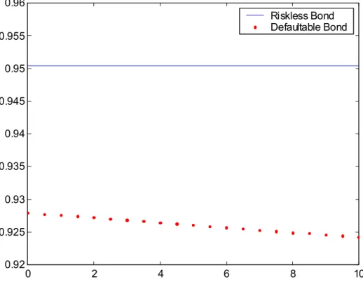
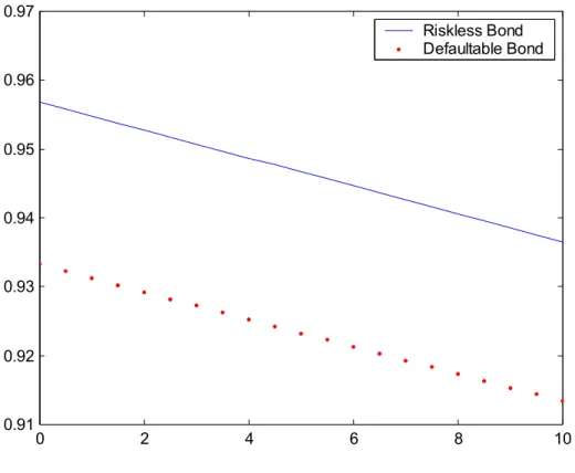
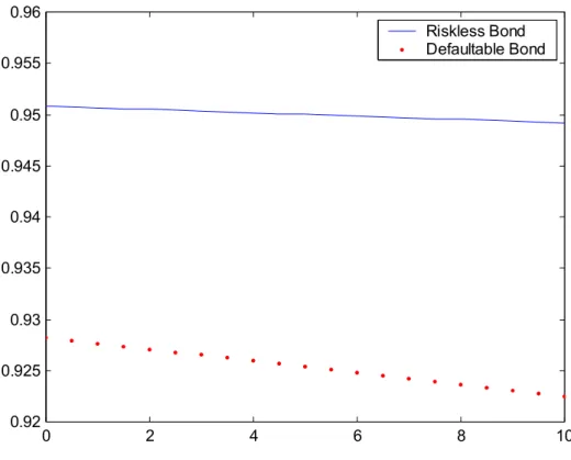
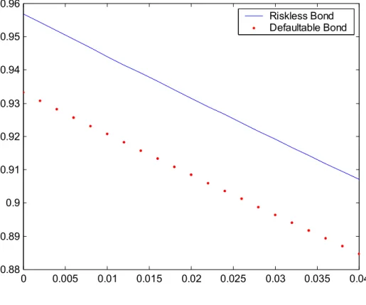
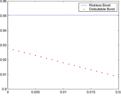
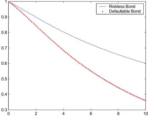
Figures 1-5 show how the values of the riskless and the defaultable bond change with respect to changes in some of the parameters. As the intensity of the any type of jump in this model increases, one would expect a reduction in bond prices due to a higher rate of discounting. In fact this is exactly what we observe except that the riskless bond value is not influenced by changes in spread jump intensity or size which is obvious. Even the defaultable bond, however, is not very sensitive to changes in the intensity of credit spread jumps. It seems that the jumps in interest rates are more important to the valuation of defaultable bonds than the jumps in the credit spread itself, and this is so whether one considers the effects of intensity or jump sizes. This can be deduced from the slopes of the dotted lines in figures 1,2,4, and 5. Figure 6 depicts the values of the riskless and the defaultable bond with respect to maturity. One can observe that the difference in their values increases as maturity increases, which is to be expected since the defaultable bond becomes more and more
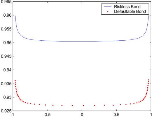
likely to default as time passes. Figure 7 shows the relation between bond values and the correlation of riskless interest rate and credit spread changes. The correlation coefficient is perturbed by varying the values of the parameter ρ in the range [-2,2] while keeping the current values of the state variables and other parametersfixed. It can be seen that the correlation coefficient does not affect neither bond’s value over a wide range. As the correlation gets near to -1 or 1, however, there is a substantial increase in the value of the both riskless and defaultable bonds. At times of market turmoil, correlation is driven by in the changes of not one parameter only, but in several parameters. Moreover, the state variables may also change drastically. To make things worse, even the whole model driving security values may change. Hence, the analysis concerning correlation in this paper is only suggestive, and hopefully is a precursor to full-fledged studies on the issue of correlation.
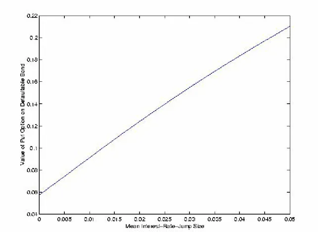
The next series offigures are concerned with the put option on a defaultable bond. In Figure 8 we observe that the value of the put option is actually more sensitive to the intensity of jumps in credit spreads than that of the jumps in interest rates, which may, at a first glance, appear to be contradictory with figures 1-3. Note that although an increase in interest rate jump intensity would decrease the value of the defaultable bond, thus increasing the value of the put option; higher interest rates would also mean higher discounting of the payoff thus reducing the value. The results so far indicate that although one may perhaps justify ignoring small jumps in credit spreads for the valuation of bonds, this omission would lead to considerable pricing errors when one is interested in the valuation of a put option on a defaultable bond, or in any other option to generalize this insight. The interpretation of figures 9 and 10 is straightforward in that any increase in mean jump sizes that would reduce the value of the underlying bond, is likely to increase the value of the put option. Figure 11 shows the value of the put option with respect to correlation.10 The observation here is that as the correlation gets near to -1 or 1 the value of the put option becomes smaller as the value of the underlying bond increases. At the most extremes, however, there is an increase in the value of the option. It remains to be seen whether this is an artifact of parameter over-perturbation. The interesting result is that the put option has its highest value for a correlation coefficient near zero. This makes sense as well since the underlying bond value is lowest around that range. Figures 12-14 display the results for the call option on credit spread. As expected, an increase in spread jump intensity and/or size increases the value of the call option while an increase in the same parameters for the interest rate jump decreases its value. This is because, unless the cash multiplier Q depends on the level of interest rates, the riskless interest rate serves only for discounting purposes for this type of derivative. It is also apparent that the value of the call option is much more sensitive to jumps in credit spreads rather than those in the riskless interest rate, suggesting that, in this case, discounting is of a secondary importance compared to the magnitude of the option payoff. In addition, as the level above which we would like to insure increases (which means we are willing to absorb most of the credit risk ourselves) the value of the call option should decrease. This is observed in Figure 15. The value of the call 10Thisfigure, along with most others, has been obtained by evaluating the relevant function over a small number of points. It has not been smoothed by interpolation to preserve its original shape.
option with respect to correlation is shown in Figure 16. It is evident that correlation does not influence much the value of the call option on credit spread. The payoff of this option is determined by how much the current level of the credit spread exceeds the given threshold. The parameter ρ does not affect this payoff. Hence perturbing
ρ has an effect on the value of the call option only through its slight influence on the riskless interest rate, that is, through discounting. The next set of figures are concerned with the spread option. In Figure 17, it can be observed that an increase in the intensities of spread jumps, and common jumps (interest rate jumps) increase (decrease) the value of the spread option, though the reduction of value occurs at a much lower rate. This should not be interpreted as to belittle the role of interest rate jumps in general. In this specific case, the effects, on the payoffof the option, of these jumps cancel each other and only a small discounting effect remains. In other cases, payoff and discounting effects may work in the same direction. Indeed, when one considers the effects of jump sizes rather than intensities, even the small discounting effect mentioned before gets rather stronger as it is evident from Figure 18. Figure 19, in turn, backs up Figure 17 in emphasizing the role of spread jumps, in that they increase the value of the option by decreasing the value of the defaultable bond. Obviously, if one expects increasing uncertainty regarding credit spreads, the right to exchange a defaultable bond for a pre-fixed number of riskless bonds become more valuable. Figure 20 concludes our analysis of the sample credit derivatives. In this figure, it can be noted that the value of the spread option with respect to correlation is rather similar to that of bonds displayed in Figure 7. Nevertheless, to account for the sharp increases in value at both extremes of the correlation range it should be the case that the defaultable bond value increases less, relative to the riskless bond over this range, or that it is discounted even more heavily.
In this part, we interpret the results of the dynamic hedging strategies details of which have been outlined earlier in Section 3.2. We consider a trader who shorts a put option on the defaultable bond, and uses the proceeds of this sale to hedge his position. The option has six months to maturity, and a strike price of 0.95. Figure 21 displays the results when he ignores the correlation. In Figure 22, he ignores credit risk altogether and uses only treasury bonds for hedging. Although this may seem naive, low liquidity in defaultable corporate bonds may force the trader to do so. Whatever the reason, undertaking such an analysis is useful in terms of quantifying the effects of this inefficient hedging strategy, and emphasizing the importance of credit risk from a hedging perspective. The values displayed in these figures are average absolute hedging errors. The trader may also be concerned with the magnitude of hedging errors with respect to the initial value of the put option. The values of the put option for various combinations of correlation defining parameters are shown in Table I. Fromfigures 21, and 22, it can be noted that the hedging errors are much lower for the trader ignoring the correlation between the credit spread and the riskless interest rate compared to those of the trader ignoring credit risk altogether. In Figure 21, it is interesting to note that when ρ1+ρ2 = 0 the hedging errors are approximately zero. This makes sense since in this case the trader is essentially using the true model to hedge the option. The disparity between the true model and the model that the trader uses is largest when ρ1 +ρ2 is large. In our case, ρ1 and ρ2 are allowed to
vary between −1 and1, soρ1+ρ2 = 2is at a maximum. The hedging error for this case is largest as can be observed from Figure 21. Finally, figures 23, and 24 display the corresponding results for a put option that has a maturity of one year. As time to maturity increases the errors seem to accumulate as it implied by the figures. To resume the findings in this part: the empirical results indicate that hedging options on defaultable corporate bonds using treasury bonds (thus ignoring credit risk) may result in large hedging errors, that ignoring correlation is also likely to lead to errors, though smaller in magnitude, and that as the time to maturity of the option to be hedged increases hedging errors increase as well.
5
Conclusion
In this paper we have proposed a general framework for the valuation of default-able securities. The transform analysis used in the paper is its first application to the valuation of credit risky securities. The proposed model is a multivariate affine structure in which state variables follow jump-diffusion processes. Negative correla-tion between the credit spread and the riskless interest rate is allowed in the model, as well as time-varying conditional correlations and variances. The proposed affine structure is admissible in the sense of Dai and Singleton (1999), and allows multiple economic interpretations for the state variables. Within this framework, defaultable bonds, a put option on the defaultable bond, a call option on the credit spread, and a credit spread option are valued. Valuation of vulnerable options is discussed as well. The model is calibrated to a cross-section of bond prices and sensitivity analysis is conducted with respect to parameters defining jump terms, and correlation. The performance of dynamic hedging strategies is analysed with respect to the correlation between the credit spread and the riskless interest rate. The results obtained show that both types of jumps, spread and interest rate, can be important in the valuation of defaultable securities depending particularly on whether one is valuing a bond or an option on the bond. The effects of correlation on the values of credit derivatives are also quite context dependent. Nevertheless, thefindings indicate that particular attention should be paid for extreme correlation coefficients for all cases, since the effects on value may be enormous. The findings regarding the hedging strategies show that ignoring default risk in hedging options on defaultable bonds can lead to substantial hedging errors irrespective, largely, of the correlation structure in the true model. Errors, though smaller in magnitude, also follow if the correlation between the riskless interest rate and the credit spread is ignored.
6
References
1. Akgun, A (2000). Model Risk with Jump Diffusions. pp. 181-207 in Model Risk, (Edited by R.Gibson) Risk Publications.
2. Bakshi, G., and D.Madan (1999). Spanning and Derivative-Security Valuation. Forthcoming in theJournal of Financial Economics.
3. Bohmann, H (1970). A Method to Calculate the Distribution Function When the Characteristic Function is Known. Nordisk Tidskr. Informationsbehandling
10, 237-242.
4. Chen, R.R., and L.Scott (1995). Interest Rate Options in Multifactor Cox-Ingersoll-Ross Models of the Term Structure. Journal of Derivatives, Winter 1995, 53.
5. Cox, J.C., J.E.Ingersoll, and S.A.Ross (1985). A Theory of the Term Structure of Interest Rates. Econometrica 53, 385-408.
6. Dai, Q., and K.Singleton (1999). Specification Analysis of Affine Term-Structure Models. Working Paper, Stanford University.
7. Das, S., and P.Tufano (1996). Pricing Credit-Sensitive Debt When Interest Rates, Credit Ratings and Credit Spreads are Stochastic. Journal of Financial Engineering 5, 161-198.
8. Duffee, G (1999). Estimating the Price of Default Risk. Review of Financial Studies 12, 197-226.
9. Duffie, D (1996). Dynamic Asset Pricing Theory. Second Edition. Princeton University Press, Princeton, N.J.
10. Duffie, D., and R.Kan (1996). A Yield-Factor Model of Interest Rates. Mathe-matical Finance 6, 379-406.
11. Duffie, D., M.Schroder, and C.Skiadas (1996). Recursive Valuation of Default-able Securities and the Timing of Resolution of Uncertainty. Annals of Applied Probability 6, 1075-1090.
12. Duffie, D., and K.Singleton (1999). Modeling Term Structures of Defaultable Bonds. Review of Financial Studies.
13. Duffie, D., J.Pan, and K.Singleton (1999). Transform Analysis and Option Pricing for Affine Jump-Diffusions. Working Paper, Stanford University. 14. Heath D., R.Jarrow, and A.J.Morton (1992). Bond Pricing and the Term
Struc-ture of Interest Rates: A New Methodology for Contingent Claims Valuation.
15. Jarrow, R., and S.Turnbull (1995). Pricing Options on Financial Securities Subject to Default Risk. Journal of Finance 50, 53-86.
16. Jarrow, R., D.Lando, and S.Turnbull (1997). A Markov Model for the Term Structure of Credit Spreads. Review of Financial Studies 10, 481-523.
17. Jarrow, R., and S.Turnbull (2000). The Intersection of Market and Credit Risk.
Journal of Banking and Finance 24, 271-299.
18. Lando, D (1998). On Cox Processes and Credit Risky Securities. Review of Derivatives Research 2, 99-120.
19. Longstaff, F.A., and E.S.Schwartz (1995). A Simple Approach to Valuing Risky Fixed and Floating Rate Debt. Journal of Finance 50, 789-820.
20. Merton, R.C (1974). On the Pricing of Corporate Debt: The Risk Structure of Interest Rates. Journal of Finance 29, 449-470.
21. Milstein, G.N (1974). Approximate Integration of Stochastic Differential Equa-tions. Theory of Probability and Applications 19, 557-562.
22. Pan, J (2000). Integrated Time-Series Analysis of Spot and Option Prices. Working Paper, GSB, Stanford University.
23. Protter, P (1992). Stochastic Integration and Differential Equations. Springer-Verlag, Berlin.
24. Schönbucher, P (1998) Pricing Credit Risk Derivatives. Working Paper, Uni-versity of Bonn.
25. Shephard, N.G (1991). Numerical Integration Rules for Multivariate Inversions.
Journal of Statistical Computation and Simulation 39, 37-46.
26. Vasicek, O.A (1977). An Equilibrium Characterisation of the Term Structure.
7
Appendix
Theorem 1 Generalized Multidimensional Ito lemma: LetX = (X1, X2, ..., Xn)
be an n-tuple of semimartingales as specified in (3). Thenf(Xt, t)is a semimartingale
and, f(Xt, t) = t Z 0 fs(X, s)ds+ t Z 0 fX(Xs, s)·dXsc+ 1 2 t Z 0 dXsTfXX(Xs, s)dXs + t Z 0 [f(Xs+J, s)−f(Xs, s)]·dN(s) (49)
where Xc denotes the continuous part of the semimartingale, J shows a column of
the jump size matrix J, and superscript T denotes the transpose operator.
Proof. See Protter (1992).
Theorem 2 Generalised Multidimensional Feynman-Kaˇc: Let Xt be an
n-dimensional jump-diffusion (more formally, a semimartingale) process as specified in (3). The ordinary Feynman-Kaˇc theorem applies in this setting as well, taking into account some additional technicalities. That is,
Df(x, t)−m(x, t)f(x, t) +h(x, t) = 0, (x,t)∈Rn×[0, T) with f(x, T) =g(x). (50) Then f(x, t) =Ex,t T Z t ϕt,sh(Xs, s)ds+ϕt,Tg(XT) with ϕt,s = exp − s Z t m(Xu, u)du (51) iff f(x,t) is a solution to (50).
Proof. (Informal) Duffie (1996) proves the theorem for diffusions. The extension
to jump-diffusions follows by an appropriate manipulation of infinitesimal generators. Let Y(s) =f(Xs, s)ϕt,s for s∈[t, T]. Then
dYs= [Dcf(Xs, s)−m(Xs, s)f(Xs, s)]ϕt,sds+fX(Xs, s)σ(Xs, s)ϕt,sdW(s)
+ϕt,s[f(Xs+J, s)−f(Xs, s)]·dN(s) (52)
where Dc denotes the continuous part of the generator, and J, as before, shows a
yields Ex,t[Y(T)] =f(x, t) +Ex,t T Z t ϕt,s[Df(Xs, s)−m(Xs, s)f(Xs, s)]ds (53) =⇒f(x, t) =Ex,t T Z t ϕt,sh(Xs, s)ds+ϕt,Tg(XT) (54)
where in going from (53) to (54) we have used (50).
Proof of (16): For ease of notation letΨd
t,T;a=1,b=0(x, a0, b0) =φ(.)in (16). Then
φ(.) [α(t) +β(t)·x] should satisfy (11). Hence
DΨdt,T;a,b(x, a0, b0) = {Dφ(.)−r(x, t)φ(.)}[α(t) +β(t)·x] +φ(.) [αt(t) +βt(t)·x] +µ(x, t)φ(.)β(t) +β(t)φX(.)σ(x, t)σT(x, t) + L X j=1 λj(x, t) Z Ω £ φ(x+Jj, .)β(t)Jj¤dFJj(t) (55) where Dφ(.) =φt(.) +µ(x, t)φX(.) + 1 2tr £ φXX(.)σ(x, t)σT(x, t) ¤ + L X j=1 λj(x, t) Z Ω £© φ(x+Jj, .)−φ(x, .)ª[α(t) +β(t)·x]¤dFJj(t) (56) Using φ(.) = exp [α0(t) +β0(t)·x], simplifying, and utilising the affine formulations
in (4) through (8), yields the ODEs in (17), and (18).
Identification of the Riccati Equations:
For the empirical analysis we specialize the more general theoretical framework of Section 1. The benchmark model laid out in Section 3 necessitates that we rewrite the two sets of Riccati equations derived in Section 1 in terms of the benchmark model. This is done in the following. Note first that the dynamics of the three state variables in the benchmark model can be rewritten as follows:
d XX12((tt)) X3(t) = k01 k02 00 0 0 k3 θθ12−−XX12((tt)) −X3(t) dt + η01 η02 00 0 ρ 1 p X1(t) 0 0 0 pX2(t) 0 0 0 pγX2(t) dWdW12((tt)) dW3(t) + Js0(t) 00 Jsc0(t) 0 Jr(t) Jrc(t) dN λs s (t) dNλr r (t) dNλ(t) (57)
This along with (4) through (8) yield µ0(t) = kk12θθ12 0 , µ1(t) = −0k1 −0k2 00 0 0 −k3 (58) σ0(t) =03∗3, σ11(t) = η 2 1 0 0 0 0 0 0 0 0 ,σ12(t) = 00 η022 ρη02 0 ρη2 γ+ρ2 ,σ13(t) = 03∗3 (59) σ(x, t)σT(x, t) = η 2 1X1 0 0 0 η2 2X2 ρη2X2 0 ρη2X2 (γ+ρ2)X2 (60) r0(t) =r0, r1(t) = [0,1,1]; s0(t) =s0, s1(t) = [1,1,0] (61) R0(t) =r0+s0, R1(t) = [1,2,1]; (62) since R(x, t) =R0(t) +R1(t)·x=r(x, t) +s(x, t).
To obtain the ODEs in their final form we also need to compute the Laplace transform of jump sizes. This is done below by assuming normal univariate and bivariate distributions with parameters to be gleaned from the context. Define the following: Λ(u;X) = Z Ω euXdFX, (63) Λ(u, v;X, Y) = Z Ω euX+vYdFX,Y (64) Λ0(u, u0;X) = Z Ω euXu0XdFX (65) Λ0(u, v, u0, v0;X, Y) = Z Ω euX+vY(u0X+v0Y)dFX,Y (66) Λ(β01(t);Js(t)) = exp · β10(t)µJs + 1 2(β 0 1(t)) 2σ2 Js ¸ (67) Λ(β30(t);Jr(t)) = exp · β30(t)µJr + 1 2(β 0 3(t)) 2σ2 Jr ¸ (68) Λ(β10(t),β30(t);Jsc(t), Jrc(t)) = exp [β10(t)µJsc +β 0 3(t)µJrc] exp µ 1 2 £ (β10(t))2σJ2sc + (β 0 3(t))2σJ2rc ¤¶ exp (β10(t)β30(t)σJscσJrcρJ) (69)