Does data vintage matter for forecasting?

Working Papers

Working Papers

Working Papers

Working Papers

Ten Independence Mall Philadelphia, Pennsylvania 19106-1574

(215) 574-6428, www.phil.frb.org FEDERALRESERVEBANK OFPHILADELPHIA

Research Department

WORKING PAPER NO. 99-15

DOES DATA VINTAGE MATTER FOR FORECASTING?

Dean Croushore and Tom Stark Research Department

Federal Reserve Bank of Philadelphia

WORKING PAPER NO. 99-15

DOES DATA VINTAGE MATTER FOR FORECASTING?

Dean Croushore and Tom Stark Research Department

Federal Reserve Bank of Philadelphia

October 1999

We thank Jim Sherma, Bill Wong, and Bill Dalasio for their fine research assistance. We thank Athanasios Orphanides, Ellis Tallman, participants in seminars at the Federal Reserve Bank of Philadelphia, the University of Pennsylvania, the International Finance Division of the Federal Reserve Board, and George Washington University, as well as those at the Midwest

Macroeconomics meetings, the Pennsylvania Economics Association, the Federal Reserve System Committee on Macroeconomics, and the National Bureau of Economics Summer Institute, for their comments. The views expressed in this paper are those of the authors and do not necessarily reflect those of the Federal Reserve Bank of Philadelphia or of the Federal

DOES DATA VINTAGE MATTER FOR FORECASTING?

Abstract

This paper illustrates the use of a real-time data set for forecasting. The data set consists of vintages, or snapshots, of the major macroeconomic data available at quarterly intervals in real time. The paper explains the construction of the data set, examines the properties of several of the variables in the data set across vintages, and shows how forecasts can be affected by data revisions.

1

In a companion paper, we analyze the degree to which data vintage matters for the robustness of empirical studies in macroeconomics. See Croushore and Stark (1999).

2 _{In this discussion of the literature, we are examining only the use of real-time data in creating}

forecasts or forecasting models, and thus we’re ignoring the voluminous literature on using real-time data to evaluate forecasts, which is standard in that literature (see, for example, Zarnowitz and Braun (1993) or Keane and Runkle (1990)). Evaluating forecasts that were made in real time (such as those collected in the Survey of Professional Forecasters or the Livingston Survey) requires a much smaller real-time data set, since one needs only one data point each period. But creating ex-post real-time

DOES DATA VINTAGE MATTER FOR FORECASTING?

I. INTRODUCTION

In creating models to use for forecasting, economists use the most recent vintage of historical data available to them to develop and test alternative models. They often compare the forecasts from a new model to forecasts from alternative models, or to forecasts that were made by others in real time. However, since the analysis of the new forecasts is based on the final, revised data, rather than the data that were available to economic agents who were making forecasts in real time, the results of such exercises may be misleading.

To avoid such problems in creating forecasting models, we have developed a data set that gives a modeler a snapshot of the macroeconomic data available at any given date in the past. We call the information set available at a particular date a “vintage,” and we call the collection of such vintages a “real-time data set.”

This paper explains the reasons for the construction of this data set, describes the data set, and shows the extent to which the data vintage matters for creating forecasting models.1

There have been relatively few studies that use real-time data to analyze forecasting models.2 _{The seminal study on real-time analysis is that of Diebold and Rudebusch (1991), who}

movements of industrial production in real time than it does after the data are revised. In support of this result, Robertson and Tallman (1998a) show that a VAR that uses real-time data from the index of leading indicators produces no better forecasts for industrial production than an AR model using just lagged data on industrial production. However, they also show that the leading indicators may be useful in forecasting real output (GNP/GDP) in real time. Some

additional research uses real-time data to compare alternative forecasting methods. Robertson and Tallman (1998b) use a real-time data set to evaluate alternative VAR model specifications for forecasting unemployment, inflation, and output growth. Koenig and Dolmas (1997) develop a method for forecasting real output growth using monthly data based on real-time analysis. A further development of that idea in a paper by Koenig, Dolmas, and Piger (1999) examines the question of what sets of real-time data forecasters should use: the fully revised series available at each date, or some unrevised series of initial releases, again in the context of forecasting real output growth.

In creating our real-time data set, our goal is to provide a basic foundation for these types of forecasting studies by allowing researchers to use a standard data set, rather than collecting real-time data themselves for every different study. We begin by providing details about the data set in section II, including a discussion of how it was constructed, which variables are available for the full time period and which are incomplete, and how the data set was checked for quality. In section III, we examine several different variables, showing the degree to which the data are affected by revisions. Section IV examines how forecasts of different types may be sensitive to the choice of data vintage. We draw conclusions from these results in section V.

3

Why the middle of each quarter? Because one of the original motivations for this project came from research on the forecast efficiency of the Survey of Professional Forecasters, whose

forecasters make their forecasts in the middle of each quarter.

4 _{More precisely, there are two data sets at each date, one containing quarterly variables, such as real}

GDP, and another containing monthly variables, such as the unemployment rate.

II. THE DATA SET

In concept, a real-time data set is simple—one simply must enter old data into

spreadsheets. But in reality, producing the real-time data set required a substantial amount of digging through old source data and figuring out what data was available at what time, a procedure that wasn’t trivial, considering the lack of documentation for much of the data. As a result, the data-collection phase of this project has been going on for the past eight years.

We now have a listing of the data as it existed in the middle of each quarter (on the 15th day of the month, to be precise), from November 1965 to the present.3 _{For each vintage date, the}

data set shows you data identical to what you would have seen in published sources at that time. So, for example, if you want to know what the data looked like on August 15, 1968, you’d simply need to pull down our data set and look at the vintage for August 1968, and you would find the relevant data—a time series for each variable from the first quarter of 1947 to the second quarter of 1968.4

The variables included in the data set are nominal and real GNP (GDP after 1991); the components of real GNP/GDP, including total personal consumption expenditures (also broken down into its components: durables, nondurables, and services), business fixed investment, residential investment, the change in business inventories, government purchases (government consumption and government investment since 1996), exports, and imports; the chain-weighted

5 _{The consumer price index is available on a seasonally adjusted basis only in the more recent data}

sets. However, since the seasonally unadjusted CPI series is not revised, it can be used without concern about revisions. For complete notes on all the variables and any missing data, see the documentation files on our web page, ZZZSKLOIUERUJSDJHDVS"SDJH IRUHFDVWUHDO.

GDP price index (since 1996); the M1 and M2 measures of the money supply; total reserves at banks (adjusted for changes in reserve requirements); nonborrowed reserves; nonborrowed reserves plus extended credit; the adjusted monetary base (the reserves measures and monetary base measures are from the Federal Reserve Board, not the versions from the St. Louis Fed); the civilian unemployment rate; the consumer price index (CPI-U); the three-month T-bill interest rate; and the 10-year Treasury bond interest rate. Even though the interest-rate variables are never revised, they’re included for completeness. The other variables are revised to some degree over time, though some, like the CPI, are revised only through changes in seasonal adjustment factors or changes in the base year. Note that the data set includes the GDP price index after 1996, but doesn’t include any type of price deflator prior to 1996, because such a deflator can be constructed by taking the ratio of nominal GNP/GDP to real GNP/GDP. The data set is mostly complete, but some data are missing for the money stock, monetary base, and reserves variables.5

Though the project of collecting these data seems simple, it turned out that finding old data is not easy. Further, since the critical element for economic research is the timing of the data (was it released during the second week of February or the third?), we tried very carefully to include in the data set only the data we knew were available at the time. In many cases data were revised, but the publications that detailed the revisions did not always say when the data were made available. So it took a substantial amount of effort to figure out exactly what data should have been, or should not have been, included in each vintage. A comprehensive set of notes

about the data set is available to help researchers understand our conventions on including or excluding particular data. Also, some of the data have been collected in real time since this project began in 1991, though the scope of the project has expanded since that time.

Who did all this work? Some of it was done over the last five years by a small army of undergraduate students working as interns. From Princeton University: Michael Hodge, Ron Patrick, Adam Stark, Jason Harvey, Jake Erhard, Keith Wilbur, and Andrew Stern. From the University of Pennsylvania: Peter High, Lisa Forman, and Bill Wong. However, from 1997 to 1998 the lion’s share of the work was done by Bill Wong, who hammered the data set into shape under the supervision of one of the authors, Tom Stark. Our thanks to all these wonderful students who produced a high-quality product!

After entering all the data into a set of database worksheets, we ran a number of editing checks to try to ensure the quality of the data. In some cases this was easy. For example, we made sure that the sum of the components of real GNP added up to total GNP in at least two vintages each year. In other cases, where there was no adding-up constraint, we plotted growth rates of the variables to ensure that they looked sensible. This helped tremendously in finding typos in the data set.

Where can you find these data? The data set is easily accessible on the Philadelphia Fed’s web site at KWWSZZZSKLOIUERUJSDJHDVS"SDJH IRUHFDVWUHDO. From links on that web page, you can

download the data, read documentation about the data, and find out when new data will become available. We plan to add new vintages shortly after the 15th day of the middle month of each quarter.

6 _{See Croushore and Stark (1999) for a similar analysis of the revisions to nominal output, real}

consumption spending, and the price level.

III. DATA REVISIONS

We know that the economic data are revised, but are such revisions large enough to worry about? To investigate this question, we’ll look at a few selected variables: real output, business fixed investment, residential fixed investment, consumption spending on durable goods, and consumption spending on nondurables and services.6

First, to see how much the data vintage matters for fairly long horizons, we’ll examine five-year average growth rates. We look at the annual average growth rate over five-year periods in Table III.1 for data from vintages (hereafter called “benchmark vintages”) dated November 1975, 1980, 1985, 1991, 1995, and 1998. These vintages were chosen because, except for the 1998 vintage, they were the last vintages prior to a comprehensive revision of the national income and product accounts; the November 1998 vintage was the latest available data vintage when the empirical work in this article was completed.

When the government made comprehensive revisions to the national income data following our benchmark vintage dates, they often made significant changes to the data,

including changing the definitions of variables and incorporating new source data. The base year was changed for real variables in January 1976 (from 1958 to 1972), in December 1985 (from 1972 to 1982), in late November 1991 (from 1982 to 1987), and in January 1996 (from 1987 to 1992). As a result, some of the differences across the benchmark vintages we look at (1980, 1991, 1995, and 1998) incorporate base-year changes, which affect real variables. Most importantly, since the base-year changes in 1976, 1985, and 1991 used the old fixed-weighted

7 _{We could create a data set with all GNP data, but GNP data are no longer released at the same time}

as the headline number (GDP); so the timing in all the data sets would change.

index methodology, the change of base year alters the timing of substitution bias; this bias is large for dates further away from the base year.

There is a potentially significant change in one of our variables across the benchmark vintages. The real output variable is GNP before 1992, but GDP during and after 1992. Our data set is consistent with the “headline” variable, but users need to be aware of this change, since the differences between GNP and GDP are not random; they are persistent in sign. So some of the differences across vintages in real output arise because of this definitional change.7 A

major change in the methodology of the national income accounts arose in 1996, when the government switched from fixed-weighted indexes to chain weighting, to eliminate the substitution bias. Under the fixed-weight methodology, such a change in the base year led to significant changes in the growth rates of real variables, often with large changes for years in the distant past. Under chain weighting, however, a change of base year has no impact on the growth rates of real variables from long ago.

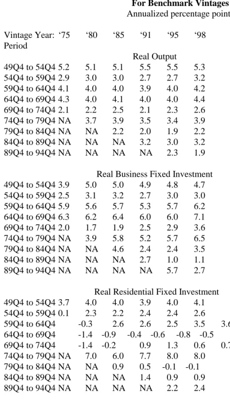
As we look across the columns of Table III.1, we can see how the five-year annual average growth rate has changed across benchmark vintages. For real output, the vintage makes a difference, especially when the base year is changed. Especially large changes show up in moving from the 1985 to the 1991 benchmark vintage (reflecting the base-year shift of December 1985) and moving from the 1995 to the 1998 benchmark vintage (reflecting the move to chain weighting in 1996). But those differences in real output growth are tiny compared with what we see for various components of output. The growth rates for business fixed investment have

changed dramatically across vintages. For example, business investment grew 3.9 percent per year in the first half of the 1950s, according to the 1975 benchmark vintage, but grew 5.0 percent per year according to the 1980 vintage. Even more dramatic was the slowdown in the measured growth rate in the first half of the 1990s, from 5.7 percent in the 1995 vintage to just 2.7 percent in the 1998 vintage (thanks, in large part, to the switch to chain weighting and the impact that had on investment in producers’ durable equipment, especially for computers). Other dramatic changes in the five-year growth rates across vintages can also be observed. Looking at

residential investment, we also see some fairly dramatic changes across vintages, especially for time periods like the early 1970s, when initial data showed negative growth; however, later vintages show growth rates as high as 1.3 percent, and 1998 vintage data show a growth rate of 0.7 percent. Consumer spending on durables is also quite volatile as measured across the

benchmark vintages, especially in the second half of the 1950s and again in the second half of the 1960s. However, the growth rates of nondurables and services don’t show much variation across vintages.

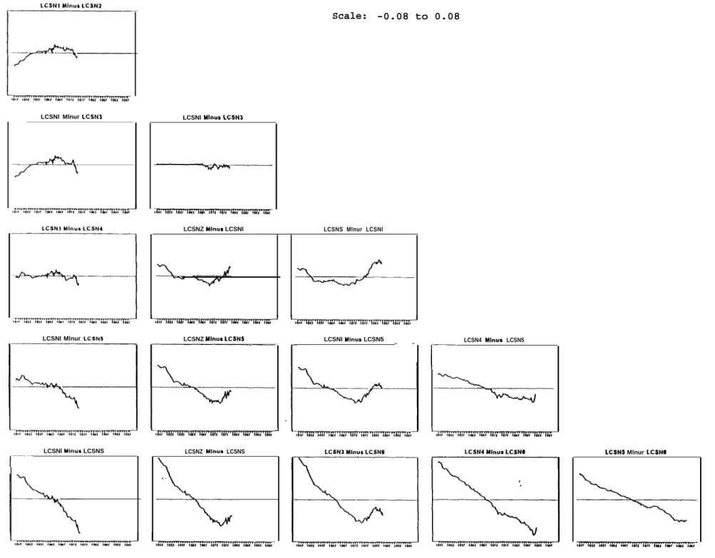
One way to examine how revisions affect the data is to plot differences in the data across vintages for the same date. Figures III.1 to III.5 show plots of the differences between the log levels of the variables, with the mean difference (over the common time period) subtracted, because it reflects mainly base-year changes. Let X(t,s) represent the level of a variable for time t in vintage s. We plot, for each date t that is common to vintages a and b, the value of Z_t/ log

8 _{Since we’ve removed the mean, we won’t capture any mean shifts in variables, but those are}

illustrated in Table III.1.

[X(t,a)/X(t,b)] - m / log [X(t,a)] - log [X(t,b)] - m, where m is the mean of log[X( ,a)/X( ,b)] over the largest sample of contained in both vintages, and where b is a later vintage than a.8

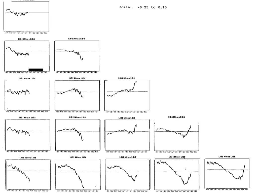
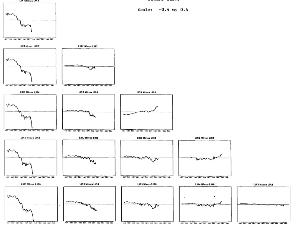
In the figures, the first column of plots compares the first benchmark vintage (a = 1975) to each later benchmark vintage. So, the upper left plot is the second benchmark vintage (b = 1980) compared to the first; the plot below that compares the third benchmark vintage (b = 1985) to the first; and so on. The second column does the same for the second benchmark vintage (a = 1980), and so on, and the final column, which has just one entry, compares the fifth benchmark vintage (a = 1995) to the sixth (b = 1998). The notation on each plot follows the convention Lz#, where L means the logarithm of the variable, z represents the variable (z=Y for real output, z=IB for business fixed investment, z=IR for residential fixed investment, z=CD for consumption of durables, and z=CSN for consumption of services and nondurables), and where # represents the benchmark vintage, with #=1 for the November 1975 vintage, #=2 for 1980, #=3 for 1985, #=4 for 1991, #=5 for 1995, and #=6 for 1998.

If you look at plots on the main diagonal of the figures, you’re comparing adjacent benchmark vintages. The plots below the main diagonal show comparisons across two or more benchmark vintages. Each plot shows dates along the horizontal axis from 1947Q1 to 1998Q3. The last data point plotted is 1975Q3 in column 1, 1980Q3 in column 2, 1985Q3 in column 3, 1991Q3 in column 4, and 1995Q3 in column 5. The vertical axis in each plot is listed at the top of each figure; these are demeaned log differences.

Three major features of the plots are apparent: (1) trends; (2) spikes; and (3) other deviations from a linear trend. First, the dominant feature of the plots is the presence of trends. A downward tilt means that later data points were revised upward relative to earlier data, reflecting faster trend growth; similarly, an upward tilt means that later data points were revised downward relative to earlier data. Second, a spike in a plot means that data for a particular date or series of dates were revised significantly in one direction relative to other dates in the sample. The third source of difference in the plots is the presence of long-lived deviations from a linear trend (or, when no trend is evident, from zero), suggesting that there are low frequency

differences between vintages. Taken together, the plots point to cross-vintage differences at many frequencies.

In Figure III.1, the effects of substitution bias on real output growth rates are apparent. The real output series, especially moving from vintage 3 to vintage 4, is tilted upward, because the fixed-weight method using the 1982 base year greatly changes the relative pricing

relationships between energy and other goods. Thus, the plot is tilted, as even data from long before were affected significantly. But moving from vintage 5 to vintage 6 reverses that effect, thanks to chain weighting. Notice also that the movement from GNP to GDP (from vintage 4 to vintage 5) didn’t cause much effect.

In Figure III.2, showing business fixed investment, the most striking result is the steepness of the plots in the bottom row. This represents changes in methodology when chain-weighting was introduced in 1996. As a result, changes to investment spending estimates were particularly pronounced, because of large changes in the price indexes for investment in

9 _{For more on these issues, see Landefeld and Parker (1995, 1997).}

technology (especially computers), and hence in the real value of investment.9 In addition, the

changes in the measurement of investment spending when benchmark revisions occur (columns 1, 3, 4, and 5) are remarkable, especially because they are nonlinear. They come from a variety of sources, including new data from censuses, changes in estimated prices, and changes in procedures for calculating values. This suggests that, in analyzing forecasts, one should be very careful about what vintage of the data one uses as “actual,” since redefinitions, changes in methodology, and changes in relative prices seem to have dramatic effects on both the levels and the growth rates of business fixed investment.

Figure III.3 shows that residential investment has also been strongly affected by the revision process. No doubt this is because of changes in the methods by which residential investment is calculated. For example, in the 1976 benchmark revision (reflected in the upper left plot), housing gets revised up dramatically, thanks to new source data on estimates of multiunit structures, changes in price indices for new construction, and the reclassification from consumption to investment of some items (mobile homes and consumer durables installed in rental dwellings).

Figure III.4 shows real consumption on durables is strongly affected by some revisions, but less so by others. As is the case with some of the other plots, chain-weighting leads to the opposite tilt direction of weighting, because of distortions of relative prices under fixed-weighting. In the first column, the decline in durables from the benchmark revision came about from the reclassification of some items from consumption to residential investment (described above), plus reclassification of a portion of autos from consumption to business investment

(depending on personal versus business ownership). In the fourth column, the declines in the growth rates of durables arise because of changed depreciation assumptions, new source data, and quality adjustments. And in the last column, it’s mostly the change to chain weighting that affects the pattern of revisions. Chain-weighting reverses some of the earlier effects of fixed-weighting, so the lower left-hand plot is basically flat, though other plots have a substantial tilt to them.

Compared to the other figures, the plots for consumption of nondurables and services (Figure III.5) are quite tame. Note that the scale is smaller than in most of the other figures.

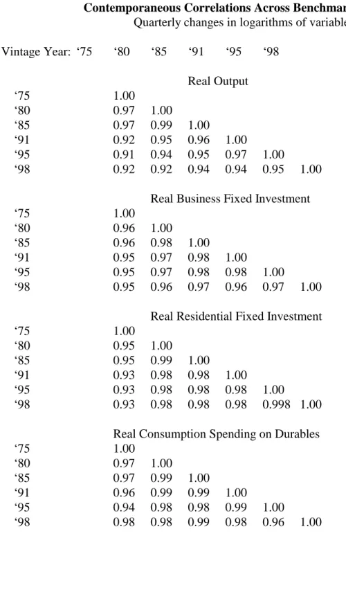
The differences observed in Figures III.1 to III.5 across vintages point to the fact that the data are revised substantially. Cross-vintage correlations of the quarterly log differences in the variables (Table III.2) aren’t as high as might be expected, given that the observations are measures of the same variable, suggesting that one’s interpretation of the data depends a lot on the vintage being examined.

Having documented that data revisions are potentially large for a variety of variables, we now pose the question: do such revisions matter for forecasting?

IV. HOW VINTAGE MATTERS FOR FORECASTING

To illustrate how the data vintage matters in forecasting, we run some simple empirical exercises. We estimate and forecast real output growth with an ARIMA model, with a univariate Bayesian model, and with a multivariate quarterly Bayesian vector error-correction (QBVEC) model and compare the results based on using real-time data to those based on current-vintage data. We have complete data on all variables used in the three models in real-time data sets with

vintages beginning in February 1975 and data in each vintage data set going back to 1959, the limiting variable being M2 in the QBVEC model. We proceed in the following manner: (1) estimate a model for real output growth using data from the first quarter of 1959 through the fourth quarter of 1974 that was known in February 1975; (2) forecast quarter-over-quarter real output growth for the current quarter and the following four quarters (from the second quarter of 1975 to the first quarter of 1976), then form a four-quarter average growth rate forecast over that time span; (3) repeat parts (1) and (2) in a rolling procedure, going forward one quarter each step; and (4) calculate the forecast errors based on the four-quarter-average forecasts. We follow this procedure once using the real-time data set (for which data revisions are possible as we roll forward each quarter), and a second time using today’s data (vintage November 1998, which contains no data revisions as we roll forward each quarter).

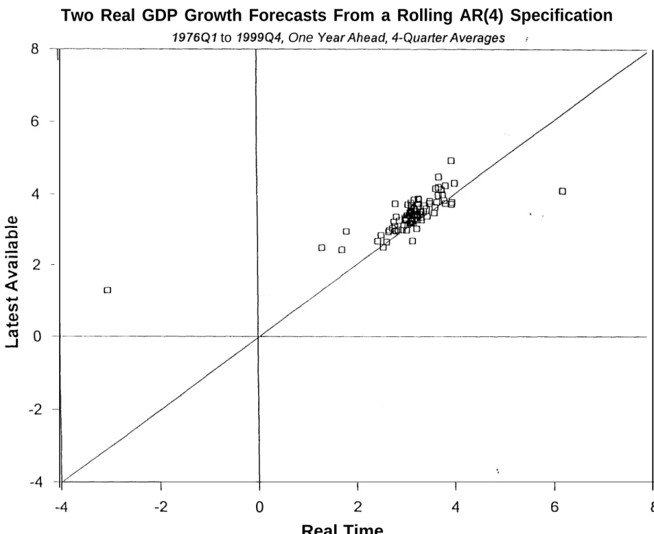
When we run this exercise first with an AR(4) model on real output, we find that the two forecasts look somewhat different over time, but not dramatically so (Figure IV.1). There’s certainly a lot more variation in the actual data than there is across forecasts, as can be seen in Figure IV.2. A scatter plot of the two forecast series shows a positive relationship between the two sets of forecasts, but there are systematic differences between the forecasts (Figure IV.3). Evidently, the vintage of the data matters even for such simple forecasts as these AR(4) forecasts. Taking the November 1998 vintage data set as representing the actual value for the data, we show in the first two rows of Table IV.1 that the root-mean-square-forecast error is not very different when forecasts are based on real-time data as opposed to final revised data. That’s actually quite surprising because it says that having today’s vintage gives no better forecast performance than having available just real-time data, when the goal is to forecast the data as

10 _{Unlike Litterman, we estimate the model in first differences, thereby imposing with certainty a unit}

root on the process.

they appear today; or it may simply mean that forecasting a variable such as real output growth using time-series methods isn’t a very productive enterprise; all forecasts are pretty much returns to trend.

An alternative forecasting method, which helps to filter shocks (or revisions) to the data, is to use Bayesian methods for estimation. Following Litterman (1986), we forecast output growth with a Bayesian AR(4) process, with standard Minnesota priors.10 This treatment means

our prior is that real output is represented by a random walk with drift or that output growth is a constant plus white noise, but the priors are not tight. With very loose priors, we’d have the AR(4) model discussed above. If we made the priors very tight, we’d impose the random walk exactly. Instead, we choose a relatively loose value of the tightness parameter of 0.2, which is the standard deviation around our prior that the coefficient on the first lag of output growth is zero. Standard deviations on our priors for the remaining coefficients fall with the lag.

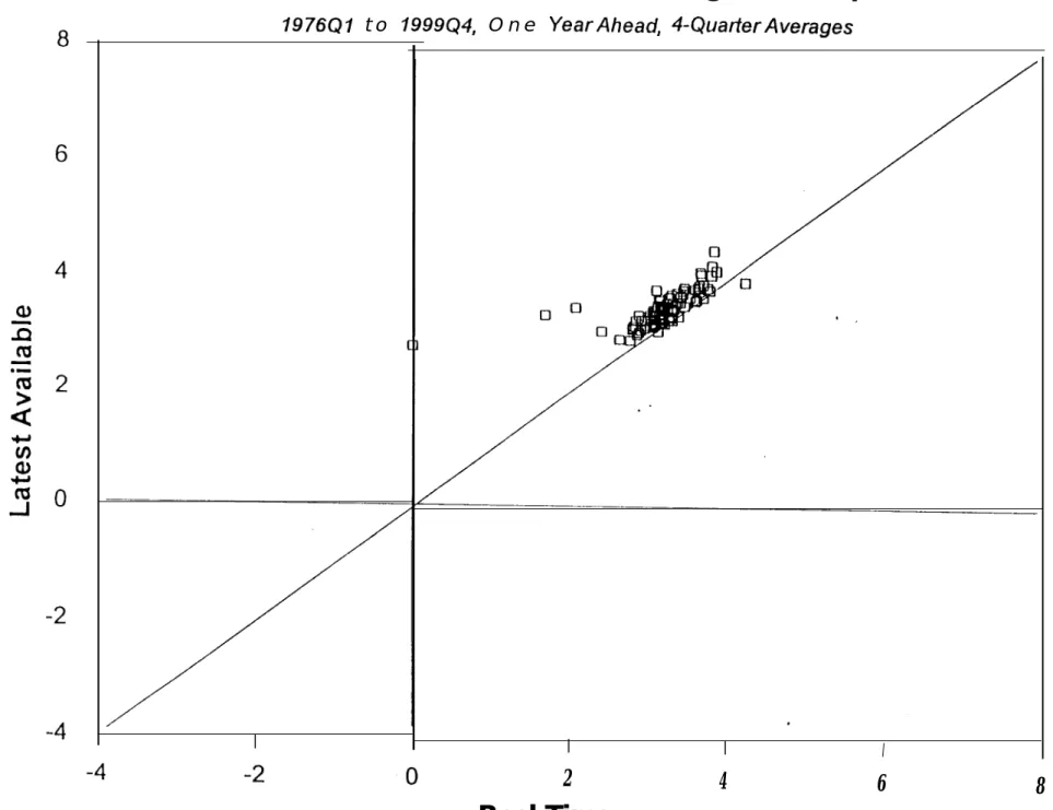
Following the same procedure as in the non-Bayesian AR(4) exercise above, we obtain somewhat different results. Figure IV.4 shows some substantial differences between the forecasts made with real-time data and those made with today’s data. Those differences in forecasts relate more to the estimate of the average growth rate of real output (in levels of real output, the drift), as Figure IV.5 shows. The scatterplot in Figure IV.6 shows that the forecasts are more tightly clustered than they were in the non-Bayesian AR(4) case, but the majority are above the 45-degree line, showing persistent differences in the forecasts. Despite that, the real-time forecasts again have about the same root-mean-squared error as those made with today’s

data, even though today’s data are used as actuals in calculating the forecast error, as can be seen in Table IV.1.

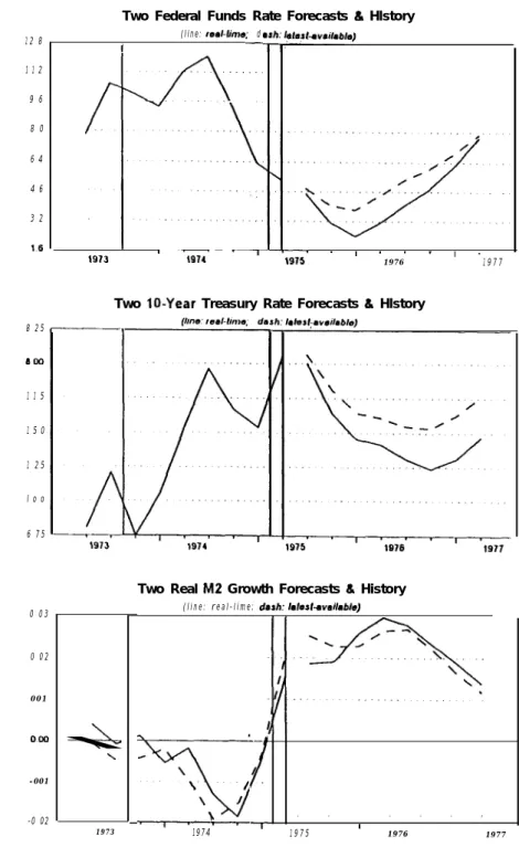
Our third forecasting exercise uses the quarterly Bayesian vector error corrections model of Stark (1998). This model was designed at the Philadelphia Fed for forecasting and for evaluating monetary policy issues. It applies Litterman’s techniques to a VAR composed of real output, the GDP price index, the federal funds rate, real import prices, the unemployment rate, real M2, and the interest rate on 10-year Treasury bonds , with 5 lags of each variable. The multivariate aspect of this model, compared with the earlier models, leads to substantially reduced forecast errors. The model differs from Litterman’s approach in two major ways: (1) it imposes unit roots in the model, which others have found improves the forecasting ability of this class of model; and (2) it adds an error-correction term consisting of the spread between the federal funds rate and the long-bond rate, with a diffuse prior. Thus, any long-run forecast obeys a cointegrating relationship between short-term and long-term interest rates. In this model, we can examine forecasts of variables other than real output.

It’s instructive to first examine a couple of episodes in which the real-time data differ substantially from today’s data. Figure IV.7 shows history and forecasts from data vintage August 1975. Solid lines to the left of the break in each line represent history as seen in real time, while the dashed lines to the left of the break are what is seen in today’s data. To the right of the break in each line are the forecasts. Note that real output growth looks substantially different today than it did in real time (the numbers on the vertical axis are log changes in the level of real output from one quarter to the next, so take the differences between the two lines and multiply by 400 to get the difference in growth rates). As a result, the forecast for real

11 _{This same pattern holds even if the univariate models take a more general ARMA form. It’s the}

use of additional variables in the QBVEC that generates the variability in the forecasts.

output growth in the future is substantially higher in real time, since the model predicts a greater rebound from a deeper recession. Note also the substantial differences in the forecast for

inflation.

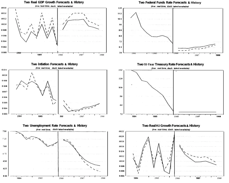
Additional examples include August 1986 (Figure IV.8) and August 1992 (Figure IV.9). In August 1986, the most recent data showed a decline in output growth and inflation, and using the real-time data, the model forecasts a rebound in output but a continued decline in inflation. Based on latest-available date, however, the path for output is stronger in the forecast, with a lower path for the federal funds rate. Similarly, in August 1992, output appeared to be growing much more slowly than it does in today’s data, resulting in substantial differences in the

forecasts, with lower output, inflation, and interest rates in the forecast based on real-time data than in the forecast that is based on latest-available data.

Looking at figures like those we used for the AR(4) model and BAR(4) model, we see that the forecasts for real output aren’t too different (Figure IV.10) except in certain periods such as 1976, when the forecasts differ by about two percentage points. The forecasts are

substantially more variable (Figure IV.11) than was the case with the other forecast models. That is, the AR(4) and BAR(4) models generate one-year-ahead forecasts that mostly represent output growth returning to trend. But the QBVEC forecasts allow for much more variation in real output over the forecast horizon because of the use of other variables.11

The real-time forecast lines up more closely (Figure IV.12) with the forecast using

the BAR(4). We can also see that although the differences between real-time forecasting and forecasting with today’s data aren’t very large for real output growth, they are substantially larger for other variables, such as inflation, as can be seen in Figures IV.13 to IV.15. Because of

changes in the methodology of measuring inflation and the relationships between other variables and inflation, the forecasts are quite different when comparing real-time forecasts to forecasts based on today’s data. The forecasts differ by as much as 3-1/2 percentage points in 1976, though most of the forecasts are within one percentage point of each other. In the scatterplot, more observations are farther off the 45-degree line than was the case for output. Thus the effects of data revisions show up more in forecasts for some variables than for others.

As with the other variables, there isn’t much difference in the root-mean-square errors, or other error measures, between using real-time or latest data. But note that the root-mean-square errors are lower for the QBVEC compared to univariate methods (Table IV.1), though the mean errors are larger in magnitude.

V. CONCLUSIONS

This paper describes a real-time data set for use in forecasting, explains how the data were put together, and shows the extent to which data revisions are potentially large enough to matter. The paper then illustrates that data revisions matter significantly for forecasting. Forecasts based on real-time data are certainly correlated with forecasts based on final data, but data revisions to real output are so large that they may cause forecasts based on current-vintage data to be considerably different from forecasts based on real-time data. This sounds a

cautionary note for studies claiming that some new, improved forecasting method beats other methods, if the study presents only evidence based on current-vintage data rather than real-time data.

Our hope is that the real-time data set presented in this paper and available on our web site will serve as a standard for forecasters.

Table III.1

Average Growth Rates Over Five Years For Benchmark Vintages

Annualized percentage points

Vintage Year: ‘75 ‘80 ‘85 ‘91 ‘95 ‘98 Period Real Output 49Q4 to 54Q4 5.2 5.1 5.1 5.5 5.5 5.3 54Q4 to 59Q4 2.9 3.0 3.0 2.7 2.7 3.2 59Q4 to 64Q4 4.1 4.0 4.0 3.9 4.0 4.2 64Q4 to 69Q4 4.3 4.0 4.1 4.0 4.0 4.4 69Q4 to 74Q4 2.1 2.2 2.5 2.1 2.3 2.6 74Q4 to 79Q4 NA 3.7 3.9 3.5 3.4 3.9 79Q4 to 84Q4 NA NA 2.2 2.0 1.9 2.2 84Q4 to 89Q4 NA NA NA 3.2 3.0 3.2 89Q4 to 94Q4 NA NA NA NA 2.3 1.9

Real Business Fixed Investment

49Q4 to 54Q4 3.9 5.0 5.0 4.9 4.8 4.7 54Q4 to 59Q4 2.5 3.1 3.2 2.7 3.0 3.0 59Q4 to 64Q4 5.9 5.6 5.7 5.3 5.7 6.2 64Q4 to 69Q4 6.3 6.2 6.4 6.0 6.0 7.1 69Q4 to 74Q4 2.0 1.7 1.9 2.5 2.9 3.6 74Q4 to 79Q4 NA 3.9 5.8 5.2 5.7 6.5 79Q4 to 84Q4 NA NA 4.6 2.4 2.4 3.5 84Q4 to 89Q4 NA NA NA 2.7 1.0 1.1 89Q4 to 94Q4 NA NA NA NA 5.7 2.7

Real Residential Fixed Investment

49Q4 to 54Q4 3.7 4.0 4.0 3.9 4.0 4.1 54Q4 to 59Q4 0.1 2.3 2.2 2.4 2.4 2.6 59Q4 to 64Q4 -0.3 2.6 2.6 2.5 3.5 3.6 64Q4 to 69Q4 -1.4 -0.9 -0.4 -0.6 -0.8 -0.5 69Q4 to 74Q4 -1.4 -0.2 0.9 1.3 0.6 0.7 74Q4 to 79Q4 NA 7.0 6.0 7.7 8.0 8.0 79Q4 to 84Q4 NA NA 0.9 0.5 -0.1 -0.1 84Q4 to 89Q4 NA NA NA 1.4 0.9 0.9 89Q4 to 94Q4 NA NA NA NA 2.2 2.4

Vintage Year: ‘75 ‘80 ‘85 ‘91 ‘95 ‘98 Period

Real Consumption Spending on Durables

49Q4 to 54Q4 4.1 3.8 3.6 3.9 4.3 3.8 54Q4 to 59Q4 3.0 2.0 2.0 2.0 1.7 2.4 59Q4 to 64Q4 6.3 5.2 5.4 4.7 4.5 6.0 64Q4 to 69Q4 7.8 7.0 7.2 6.7 6.4 7.3 69Q4 to 74Q4 1.7 2.6 2.7 2.6 2.0 2.8 74Q4 to 79Q4 NA 7.1 7.0 6.8 6.3 6.6 79Q4 to 84Q4 NA NA 4.6 4.8 4.1 4.9 84Q4 to 89Q4 NA NA NA 4.9 4.7 5.0 89Q4 to 94Q4 NA NA NA NA 4.9 3.2

Real Consumption Spending on Nondurables and Services

49Q4 to 54Q4 3.5 3.2 3.2 3.7 3.8 4.0 54Q4 to 59Q4 3.5 3.4 3.4 3.4 3.5 3.8 59Q4 to 64Q4 3.7 3.6 3.6 3.6 3.7 3.9 64Q4 to 69Q4 3.8 3.9 4.0 4.1 4.3 4.4 69Q4 to 74Q4 2.4 2.6 2.6 2.5 2.7 2.9 74Q4 to 79Q4 NA 4.0 4.0 3.5 3.6 3.7 79Q4 to 84Q4 NA NA 2.4 2.1 2.2 2.4 84Q4 to 89Q4 NA NA NA 2.9 2.9 3.2 89Q4 to 94Q4 NA NA NA NA 1.9 1.9

Table III.2

Contemporaneous Correlations Across Benchmark Vintages

Quarterly changes in logarithms of variables

Vintage Year: ‘75 ‘80 ‘85 ‘91 ‘95 ‘98 Real Output ‘75 1.00 ‘80 0.97 1.00 ‘85 0.97 0.99 1.00 ‘91 0.92 0.95 0.96 1.00 ‘95 0.91 0.94 0.95 0.97 1.00 ‘98 0.92 0.92 0.94 0.94 0.95 1.00

Real Business Fixed Investment

‘75 1.00 ‘80 0.96 1.00 ‘85 0.96 0.98 1.00 ‘91 0.95 0.97 0.98 1.00 ‘95 0.95 0.97 0.98 0.98 1.00 ‘98 0.95 0.96 0.97 0.96 0.97 1.00

Real Residential Fixed Investment

‘75 1.00 ‘80 0.95 1.00 ‘85 0.95 0.99 1.00 ‘91 0.93 0.98 0.98 1.00 ‘95 0.93 0.98 0.98 0.98 1.00 ‘98 0.93 0.98 0.98 0.98 0.998 1.00

Real Consumption Spending on Durables

‘75 1.00 ‘80 0.97 1.00 ‘85 0.97 0.99 1.00 ‘91 0.96 0.99 0.99 1.00 ‘95 0.94 0.98 0.98 0.99 1.00 ‘98 0.98 0.98 0.99 0.98 0.96 1.00

Vintage Year: ‘75 ‘80 ‘85 ‘91 ‘95 ‘98

Real Consumption Spending on Nondurables and Services

‘75 1.00 ‘80 0.92 1.00 ‘85 0.91 0.97 1.00 ‘91 0.92 0.94 0.95 1.00 ‘95 0.91 0.93 0.94 0.97 1.00 ‘98 0.91 0.93 0.94 0.96 0.98 1.00

Table IV.1

Forecast Errors from Rolling Regressions

Forecast Horizons 1976Q1 to 1998Q3 Four-quarter average forecasts of real output

Mean Root

Mean Absolute Mean Square

Forecast Data Set Error Error Error

AR(4) Real Time -0.19 1.74 2.49

November 1998 -0.48 1.70 2.40

BAR(4) Real Time -0.24 1.67 2.35

November 1998 -0.54 1.67 2.34

QBVEC Real Time -0.70 1.41 1.90

REFERENCES

Croushore, Dean, and Tom Stark. “A Real-Time Data Set for Macroeconomists: Does the Data Vintage Matter?” Forthcoming, 1999, Federal Reserve Bank of Philadelphia Working Paper series.

Diebold, Francis X., and Glenn D. Rudebusch. “Forecasting Output With the Composite Leading Index: A Real-Time Analysis,” Journal of the American Statistical Association 86 (September 1991), pp. 603-10.

Keane, Michael P., and David E. Runkle. “Testing the Rationality of Price Forecasts: New Evidence From Panel Data,” American Economic Review 80 (1990), pp. 714-35. Koenig, Evan F., and Sheila Dolmas. “Real-Time GDP Growth Forecasts,” Federal Reserve

Bank of Dallas Working Paper 97-10, December 1997.

Koenig, Evan F., Sheila Dolmas, and Jeremy Piger. “The Use and Abuse of ‘Real-Time’ Data in Economic Forecasting,” Federal Reserve Bank of Kansas City, manuscript, September 1999.

Landefeld, J. Steven, and Robert P. Parker. “Preview of the Comprehensive Revision of the National Income and Product Accounts: BEA’s New Featured Measures of Output and Prices,” Survey of Current Business, July 1995, pp. 31-8.

Landefeld, J. Steven, and Robert P. Parker. “BEA’s Chain Indexes, Time Series, and Measures of Long-Term Economic Growth,” Survey of Current Business, May 1997, pp. 58-68. Litterman, Robert B. “Forecasting with Bayesian Vector Autoregressions--Five Years of

Robertson, John C., and Ellis W. Tallman. “Data Vintages and Measuring Forecast Model Performance,” Federal Reserve Bank of Atlanta Economic Review (Fourth Quarter 1998a), pp. 4-20.

Robertson, John C., and Ellis W. Tallman. “Real-Time Forecasting with a VAR Model,” Manuscript, Federal Reserve Bank of Atlanta, November 1998b.

Rudebusch, Glenn D. “Do Measures of Monetary Policy in a VAR Make Sense?” International

Economic Review 39 (1998a), pp. 907-31.

Stark, Tom. “A Bayesian Vector Error Corrections Model of the U.S. Economy,” Federal Reserve Bank of Philadelphia Working Paper 98-12, June 1998.

Zarnowitz, Victor, and Phillip Braun. “Twenty-Two Years of the NBER-ASA Quarterly Economic Outlook Surveys: Aspects and Comparisons of Forecasting Performance,” in James H. Stock and Mark W. Watson, eds. Business Cycles, Indicators, and Forecasting. Chicago: University of Chicago Press, 1993, pp. 11-94.

LYl Mlnur LY2 _{Figure III.1}

Scale: -0.08 to 0.08

LYI Minus LY4

LYI Minus l.YS

I

LYl Mlnur LYI

r

LY2 Minus LY4

I

LY3 Mlnur LY4

LIB1 wnur LIB2

I

-%

LIB1 hunus LIB4

I

LIB2 Minus LIB3

LIB2 Minus LIB4

LIB2 Mlnur LIB5

LlB2 Minus LIB0 I

Figure III.2

Sdale: -0.25 to 0.15

LIB1 MLnur LIB4

&

LIE3 Minus LIB0

LIB4 Mlnur LIB5

I I

LIAl Minus UR2 ---I

LlRl Mlnur LlRl

I

LlRl Minus LIRS

LIRl Mlnur LIRS

Figure III.3

Scale: -0.4 to 0.4

LlR2 Mlnus LIRJ

LlR2 Yinus LIRI

LlR2 Hlnw LIRI

LIRl Hlnus LIR4

--Lx7

LCD1 Mlnur LCD2 -- ---I Figure III.4 Scale: -0.20 to 0.20 LCD$ Minus LCD4 LCD! Mlnur LCD6 LCD2 Minus LCD3 141 I , I I I #-maw LCD2 Mlnur LCD4 LCD2 Minus LCD5 LCD2 Mlnur LCD8 LCD3 Mlnur LCD4 LCD1 Mlnur LCD5 --_-~

1

Figure III.5

Scale: -0.08 to 0.08

LCSNl Ylnus LCSN3 LCSNl Mlnur LCSN3

LCSNZ Minus LCSNI LCSNS Mlnur LCSNI

LCSNZ Minus LCSN5

LCSNI Mlnur LCSN5 LCSNI Hlnur LCSN5

- - LCSN4 Minus LCSN5 r i LCSNZ Mlnw LCSNS ,. ‘\,,

I----

6 4 2 0 -2 -4 -6 F i g u r e I V . 1

A Comparison of Two Real GDP Forecasts From A Rolling AR(4) Model One Year Ahead, Four-Quatier Growth Rates

- RealTIme Lalesl Available

A Comparison of Two Forecast Errors From A Roiling AR(4) Model

Actual Minus Predicted ’ I

i8 1961 1964 1967 1970 1973 1.05 0.70 0.35 0.00 -0.35 -0.70 -1.05 -1.40 -1.75 - R e a l Tlme - - _{Lalesl Available} 1 9 9 7 2 0 0 0

Difference Between Errors

Real Time Minus Latest Available

. . ,t . . ..JI

, * ,I

L ”

10.0 7.5 5.0 2.5 0.0 -2.5 -5.0 10.0 2.5 -2.5 F i g u r e I V . 2

Actual (line) & Predicted (dash) Real GDP Growth: Real Time

One Year Ahead, Four-Quarter Growth Rates, AR(4) ’

,~,~,~,-,‘,~,~,‘l~l’l~l’l~l’l~l’l’l~l’l

1961 1964 1967 1970 1973 1976 1979 1_{1982 1985 1988 1991 1994 1997 2000}

Actual (line) & Predicted (dash) Real GDP Growth: Latest Available

One Year Ahead, Four-Quarter Growth Rates, AR(4)

1

I\

/I

I I /. ‘. \ ‘I\ 1. 1 ‘I’ Y I l\l\1 IAL] 1 11 \ 1 I

I

-’

Y ” II I I’.;

\1 I III II

v

--VII/ v. w

I

\ I

Figure IV.3

Two Real GDP Growth Forecasts From a Rolling AR(4) Specification

7976Q7 to 1999Q4, One YearAhead, 4-QuarterAverages Y

Cl

:

I I I I

Figure IV.4 10.0 7.5 5.0 2.5 0.0 -2.5

A Comparison of Two Real GDP Forecasts From A Rolling BAR(4) Model

One Year Ahead Four-Quarter Growth Rates ! .'

Is2

A Comparison of Two Forecast Errors From A Roiling BAR(4) Model

Actual Minus Predicted

I I I [A

Difference Between Errors Real Time Minus latest Available

10.0 7.5 5.0 2.5 0.0 -2.5 -5.0 10.0 7.5 2.5 0.0 -2.5 -5.0 Figure IV.5

Actual (line) & Predicted (dash) Real GDP Growth: Real,Time

’ One Year Ahead, Four-Quarter Growth Rates, BAR(4)

-i. 1961 1964 1967 \ ,,I I T 1 1973

+TTrTrT

\I

Actual (line) & Predicted (dash) Real GDP Growth: Latest Available

\

,,‘,‘

,I-One Year Ahead, Four-Quarter Growth Rates, BAR(4)

I, 7, ,‘,‘,‘,‘,‘,‘,‘,

\ -

\,/---IA/w”

Figure IV.6

Two

Real GDP Growth Forecasts From a Rolling BAR(4) Specification

1976Ql t o 1999Q4, O n e YearAhead, 4-QuarterAverages

I

Figure IV.7

Two Real GDP Growth Forecasts L History _{Two Federal Funds Rate Forecasts & Hlstory}

1 9 7 6 1911

Two lnflatlon Forecasts L Hlstory Two lnflatlon Forecasts L Hlstory

(he reel-bma, dash Iaferl~vaifable) (he reel-bma, dash /.,ferl~va;fable) 0 0 3 2 0 0 2 4 0 0 1 6 OW8 0 0 0 0 - 0 0 0 8 - 0 0 1 6 -0 024 - 0 0 3 2 0 035 0 0 3 0 0 0 2 5 0 0 2 0 0 0 1 5 0 0 1 0 0 0 0 5 ash: li ( l i n e : reMime; d I -1 2 8 1 1 2 9 6 8 0 6 4 4 6 3 2 16 8 2 5 a00 1 1 5 1 5 0 1 2 5 l o o 6 7 5 0 0 3 0 0 2 001 000 -001 1933 I.19141-I..1915 . , . 1976. . . .1 9 7 7 L \-, 1913

Two l&Year Treasury Rate Forecasts L Hlstory

, ,

\

I - ‘ ’ I ’

1 9 7 4 l! 1 9 7 1

Two Unemployment Rate Forecasts U Hlstory

fhe. real-lime. derh lalesl-wsi/ab/eJ

Two Real M2 Growth Forecasts L History ( l i n e : r e a l - l i m e ; dash: I~ksf.avsi/ab/e) \ / \ / \ / 9 6 66 80 7 2 6 4 5 6 4 a \

Figure IV.8

Two Real GDP Growth Forecasts &I Hlstory Two Federal Funds Rate Forecasts & &tory

Ibm teal-lime. dash: Jalesl~v~ilabfeJ (he: mdlime. dash: lale&wai/ebleJ

0016 120 0014 0012 0010 0006 0006 0004 0002 OOOO 0011 0010 0009 0006 0007 0006 0005 0004 0003 750 7 25 700 6 75 650 625

1

Two lntlatlon Forecasts h Hlstory Two lo-Year Treasury Rate Forecasts L History

(IIIIS~ resl-lime. dash: /alesI-available)

‘\’ \

I \

\ I

_”

_\

_/\

-+-I

\\

\\

_\/

---_{1964 Lz---- 966}

I . - . 1 *

Two Unemployment Rate Forecasts EL Hlstory

dash: Ialeal~vai/ab/eJ 96 72 56 132 120 108 96 64 72 0022 0020 0016 0016 0014 0012 0010 0006 0.006 \ -_-H I. 1 - ‘7 1964 1965 I 1966 I. ‘. I, 1987 19.98 ’ 1966 1987 1988

Two Real M2 Growth Forecasts & Hlstory

(Ime. real-time; dash: Ielerf-wailab/e) I

Figure IV.9

Two Real GDP Growth Forecasts L Hlstory (he’ r e a l - t i m e ; d a s h ’ lalsrl-w~ilable)

I

Two Federal Funds Rate Forecasts h Hlstory

00140 00105 00070 0 0035 -0 oooo -0 0035 -00070 -0 0105 65 ... ... .... ... 1992 I . 1 I . 1993 1994

Two lnflallon Forecasts b Hlstory Two l( fear Treasury Flalle Forecasts U History ( l i n e . real-bme, dash: IQ/oaf-avmtlableJ

0013 0 0 1 2 0 0 1 , 0 0 1 0 0009 7 70 735 700 665 630 3 95 5 60

Two Unemployment Rate Forecasts (L Hlstory Two Real MZ Growth Forecasls 1L Hlstory

0010 0006 0006 0004 0002 0000 -0002 -0004 . _. \ \ . \ .

f’\

\ . -

_\

“\/\i

\ ? ’

\’ ’

Figure IV.10

A Comparison of Two Real GDP Forecasts From a RoHing QBVEC(5) Model

10 8 6 4 2 0 -2

--XT

One Year Ahead, Four Quarier Growth Rates

6 r 4 2 0 -2 -4 -6 1

A Comparison of Two Forecast Errors From a Rolling QBVEC(5) Model

Actual Minus Predicted ’ ,

z!I

Difference Between Errors

Real Time Minus Latest Available

I

Figure IV.11

Actual (line) & Predicted (dash) Real GDP: Real T‘ime

One Year Ahead, Four Quarter Growth Rates, QEWEC(5) 10 8 6 4 2 0 -2 -4 10 8 6

-I

I

I

I

I;,

t-I4

PAA

\\ ,-I

2;:7

‘2

I ’” I

\

$’

I ’

_{’ I}

I ’

1

-\

I

\

P

I

I

I

1976 19' tl1'11111'1'r1985 1988 31 1994 1997 2000I’I’I’I’I’I’\‘I’I’

Actual (line) & Predicted (dash) Real GDP: Latest Available

One Year Ahead. Four I Quarter Growth Rates, QBVEC(5)

‘I ‘I

15.0

12.5

10.0

-2.5

Figure IV.12

Two Real GDP Growth Forecasts From a Rolling QBVEC(5)

1976Ql to 199944, One YearAhead, 4-QuarterAverages

12 10 0 6 4 2 0 4 3 2 1 0 : -1 FT Figure IV.13

A Comparison of Two Inflation Forecasts From a Rolling QBVEC(5) Model

1’1’1’1’I’I’I’I I’

51 1964 1967 19;

One Year _-Ahead, Four Quarter Growth Rafes

v

\

I 6

.J\\

4

_;‘9;6’

A Comparison of Two Forecast Errors From a Rolling QBVEC(5) Model

‘I’I’I’I’I’I’I’I’,’

91 1994 1997 2000

I’I’I’I’I’I’I’I I ’ il 1964 1967 19;

Actual Minus Pradicled ’

- R e a l Time Lelesl Available.

.*.

,,‘I’,’ bI’[‘,‘,‘, ~‘~‘,‘,‘~‘~‘~‘~‘~‘~‘I’I’I’I’I’I’I’I’I’I’ 1973 1976 1979 1982 1985 1988 1991 1994 1997 2000

Difference Between Errors

70,

12 10 8 6 4 12 10 8 6 Figure IV.14

Actual (line) & Predicted (dash) Inflation: Real Time

One Year Ahead, Four Quarter Growth Rates. QSVEC(5)

,,‘,I,’

1 1973 1976 1979 1982 1985 1988 1

Actual (line) & Predicted (dash) Inflation: Latest Available

One Year Ahead, Four Querter Growth Reles. QBVECIS)

A

1:

l-T----II

II

I

I

I

-4

I

_I

--Al

15.0

12.5

5.0

2.5

0.0

Two Inflation Forecasts From a Rolling QBVEC(5)

7976Ql to 1999Q4, One YearAhead, 4-QuarterAverages _;

-1---/

I I _{I I}