Expectations, Shocks, and Asset Returns

Full text

(1)“Expectations, Shocks, and Asset Returns” Ricardo M. Sousa. NIPE WP 29 / 2007.

(2) “Expectations, Shocks, and Asset Returns”. Ricardo M. Sousa. NIPE* WP 29 / 2007. URL: http://www.eeg.uminho.pt/economia/nipe. *. NIPE – Núcleo de Investigação em Políticas Económicas – is supported by the Portuguese Foundation for Science and Technology through the Programa Operacional Ciência, Teconologia e Inovação (POCI 2010) of the Quadro Comunitário de Apoio III, which is financed by FEDER and Portuguese funds..

(3) Expectations, Shocks, and Asset Returns Ricardo M. Sousa London School of Economics, NIPE and University of Minho. October 30, 2007. Abstract I use the consumer’s budget constraint to derive a relationship between stock market returns, the residuals of the trend relationship among consumption, aggregate wealth, and labour income, cay, and three major sources of risk: future changes in the housing consumption share, cr, future labour income growth, lr, and future consumption growth, lrc. Using a VAR, I compute measures of expected and unexpected long-run changes of the major determinants of asset returns and …nd that: (i) cay, cday, expected lr, cr, lrc and expected longrun changes in ex-ante real returns, lrret, strongly forecast future asset returns; (ii) unexpected lrc and unexpected lrret contain some predictive power for asset returns; (iii) unexpected lr and unexpected cr do not predict future asset returns. One can, therefore, use the intertemporal budget constraint and the forecasting properties of an informative VAR to generate the predictability of many economically motivated variables developed in the literature on asset pricing. The framework presented is su¢ ciently ‡exible to accommodate the implications of a wide class of optimal models of consumer behaviour without imposing a functional form on preferences. Keywords: expectations, shocks, asset returns, wealth, income, consumption, housing share. JEL classi…cation: E21, E44, D12. London School of Economics, Department of Economics, Houghton Street, London WC2 2AE, United Kingdom; Núcleo de Investigação em Políticas Económicas (NIPE), University of Minho, Department of Economics, Campus of Gualtar, 4710-057 - Braga, Portugal. E-mail: [email protected], [email protected]. I am extremely grateful to Alexander Michaelides, my supervisor, and Christian Julliard for helpful comments and discussions. I also acknowledge …nancial support from the Portuguese Foundation for Science and Technology under Fellowship SFRH/BD/12985/2003.. 1.

(4) 1. Introduction Di¤erences in expected returns across assets are the naturally explained by di¤erences in risk and the. risk premium is generally considered as re‡ecting the ability of an asset to insure against consumption ‡uctuations (Lucas (1978), Breeden (1979), Sharpe (1964), Lintner (1965)). Despite this, di¤erences in the covariance of returns and contemporaneous consumption growth across portfolios have not proved to be su¢ cient to justify the di¤erences in expected returns observed in the U.S. stock market (Mankiw and Shapiro, 1986; Breeden et al., 1989; Campbell, 1996; Cochrane, 1996; Lettau and Ludvigson, 2001b).Additionally, Hansen and Singleton (1982) - for the consumptionbased models -, and Fama and French (1992) - for the CAPM -, show that these models have considerable di¢ culty in supporting the di¤erences in a cross-section of asset returns. As a result, the identi…cation of the economic sources of risks is still an important issue. According to canonical macroeconomic theory, aggregate consumption re‡ects the optimal choices of a representative consumer and can be explained by changes in the risk-free rate of return and in the information about current wealth, future income, and future rates of return. Whilst this theory is supported by the unpredictability of consumption growth, several studies have shown that predictable movements in aggregate consumption growth are almost uncorrelated with the risk-free rate of return and are significantly correlated with predictable changes in income, therefore, questioning its validity.1 Parker and Preston (2005) use household-level data to measure the relative importance of new information, the real interest rate, the preference for consumption, and precautionary saving in explaining ‡uctuations in aggregate consumption growth and …nd that precautionary savings play an important role in consumption ‡uctuations.2 ;3 By its turn and in the spirit of Brainard et al. (1991),4 Parker and Julliard (2005) measure the risk of a portfolio by its ultimate risk to consumption, de…ned as the covariance of its return and consumption growth over the quarter of the return and many following quarters and show that it is able to explain cross-section of asset returns.5 1 See. Flavin (1981), Shiller (1982), Hall (1988), Campbell and Deaton (1989), and Campbell and Mankiw (1989). (1994), Cochrane (1991), and Attanasio and Davis (1996) reject complete consumption insurance in the U.S.. 2 Nelson. and Rios-Rull (1994), Krusell and Smith (1998) and Gourinchas (2000) study precautionary saving in model economies. 3 See, for example, Baxter and Jermann (1999), Basu and Kimball (2000), and Ogaki and Reinhart (1998). Carroll (1997) argues that incomplete markets are an important source of bias, whilst Attanasio and Weber (1995) …nds that labor supply is an important shifter of the preference for consumption. 4 These authors show that the longer the horizon of the investor, the better the CCAPM performs relative to the CAPM. 5 The authors show that this can provide the correct measure of risk under several extant explanations of slow consumption adjustment, such as some models of (a) measurement error in consumption; (b) costs of adjusting consumption; (c) nonseparability of the marginal utility of consumption from factors such as labor supply or housing stock, which themselves are constrained to adjust slowly; or (d) constraints on information ‡ow or calculation so that household behavior. 2.

(5) The literature in asset pricing has, therefore, largely concluded that di¤erences in expected returns are not due to di¤erences in risk to consumption, but instead arise from ine¢ ciencies of …nancial markets, time variation in e¤ective risk aversion (Sundaresan, 1989; Constantinides, 1990; Campbell and Cochrane, 1999), in the joint distribution of consumption and asset returns or quite di¤erent models of economic behavior. In addition, several papers tried to shed more light on this question and many economically motivated variables have been developed to capture time-variation in expected returns and document long-term predictability.6 Lettau and Ludvigson (2001) show that the transitory deviation from the common trend in consumption, aggregate wealth and labor income, cay, is a strong predictor of asset returns, as long as the expected return to human capital and consumption growth are not too volatile. Fernandez-Corugedo et al. (2003) use the same approach but incorporate the relative price of durable goods, whilst Julliard (2004) shows that the expected changes in labor income are important because of their ability to track time varying risk premia. The nonseparability between consumption and leisure in on the basis of the work of Wei (2005), who argue that human capital risk can generate su¢ cient variation in the agent’s risk attitude to produce equity returns and bond yields with properties close to the observed in the data. Whilst the last two papers emphasize the role of human capital, others have focused on the importance of the housing market instead. Yogo (2006) and Piazzesi et al. (2007) emphasize the role of nonseparability of preferences in explaining the countercyclical variation in the equity premium.7 In the same spirit, Lustig and Van Nieuwerburgh (2005) show that the ratio of housing wealth to human wealth (the housing collateral ratio) shifts the conditional distribution of asset prices and consumption growth and, therefore, predicts returns on stocks. More recently, the focus has been directed towards the importance of long-term risk. Abel (1999) and Bansal and Yaron (2004) show that di¤erences in risk compensation on assets mirror di¤erences in the exposure of assets’cash ‡ows to consumption. Bansal et al. (2005) suggest that changes in expectations about the entire path of future cash ‡ows provide very valuable information about systematic risks in asset returns. Given the current state of the literature, one can ask the following questions: What are the major sources of risk that explain asset returns? What is the importance of long-term risk? Are we able to generate the predictability of asset returns without relying on a speci…c description of preferences? In this paper, I use the consumer’s budget constraint to derive a relationship between stock market returns, the residuals of the trend relationship among consumption, aggregate wealth, and labour inis “near-rational”. 6 See, for example, Fama and French (1988), Campbell and Shiller (1988), Poterba and Summers (1988), Richards (1995), Lettau and Ludvigson (2001, 2004). 7 Pakos (2003) argues that there is an important non-homotheticity in preferences.. 3.

(6) come, cay, and three major sources of risk: future changes in the housing consumption share, cr, future labour income growth, lr, and future consumption growth, lrc. I model the joint dynamics of changes in the non-housing consumption share, consumption growth, wealth growth, income growth, returns, consumption-wealth ratio and dividend-price ratio using a VAR and use it to obtain measures of expected and unexpected long-run changes in the major determinants of asset returns. I …nd that: (i) cay, cday, expected lr, cr, lrc and expected long-run changes in exante real returns, lrret, strongly forecast future asset returns; (ii) unexpected lrc and unexpected lrret contain some predictive power for asset returns; (iii) unexpected lr and unexpected cr do not predict future asset returns. Moreover, this work suggests that agents’expectations about long-run risk are important and that asset returns largely re‡ect that information. The results show that expectations of high future labor income, expectations of high future consumption growth, and expectations of high non-housing consumption share are associated with lower stock market returns, and low labor income growth expectations, low consumption growth expectations and low non-housing consumption share expectations are associated with higher than average real returns. Therefore, the success of lr, cr, and lrc as predictors of asset returns seems to be due to their ability to track risk premia. On the other hand, shocks to long-run expectations seem to play a negligible role as its forecasting power for current returns is, in general, very low. The framework presented is su¢ ciently ‡exible to accommodate the implications of a wide class of optimal models of consumer behaviour. Its advantage lies on the fact that it does not impose any functional form on preferences. It, therefore, shows that one can use the intertemporal budget constraint and the forecasting properties of an informative VAR to generate the predictability of many empirical proxies developed in the literature on asset pricing. The paper is organized as follows. Section 2 presents the theoretical and econometric approach. Section 3 describes the data and presents the estimation results of the forecasting regressions. Finally, in Section 4, I conclude and discuss the implications of the …ndings.. 2 2.1. Theory and Econometric Approach Deriving the Major Determinants of Asset Returns Following Campbell (1996) and Jagannathan and Wang (1996), labor income (Yt ) can be thought. of as the dividend on human capital (Ht ). Under this assumption, the return to human capital can be. 4.

(7) de…ned as: 1 + Rh;t+1 =. Ht+1 + Yt+1 : Ht. (1). Under the assumption that the steady state human capital-labor income ratio is constant (Y =H = 1 h. 1, where 0 <. h. < 1),8 this relation can be log-linearized around the steady state to get rh;t+1 = (1. h )kh. +. h (ht+1. yt+1 ). (ht. yt ) +. yt+1. (2). where r := log(1 + R), h := logH, y := logY , kh is a constant of no interest, and the variables without i h (ht+i. time subscript are evaluated at their steady state value. Assuming that limi!1. yt+i ) = 0, the. log human capital income ratio can be rewritten as a linear combination of future labor income growth and future returns on human capital: ht. yt =. 1 X. i 1 h (. yt+i. rh;t+i ) + kh :. (3). i=1. Equation (2) shows that the log human capital to labor income ration ratio has to be equal to the discounted sum of future labor income growth and human capital returns. Moreover, this equation is similar, both in structure and interpretation, to the relation between the log dividend-price ratio and future returns and dividends derived by Campbell and Shiller (1988): taking time t conditional expectation of both sides, when the log human capital to labor income ratio is high, agents should expect high future labor income growth or low human capital returns.9 De…ning Wt as aggregate wealth (given by human capital plus asset holdings), Ct as non-housing consumption, Ut as consumption of housing services, Ptu as relative price of consumption of housing services, St as non-housing consumption share,10 and Rw;t+1 as the return on aggregate wealth between period t and t + 1, the consumer’s budget constraint can be written as:11 Wt+1 = (1 + Rw;t+1 ) (Wt. Ct. Ptu Ut ) = (1 + Rw;t+1 ) Wt. Ct St. :. (4). Campbell and Mankiw (1989) show that, under the assumption that the consumption-aggregate wealth is stationary and that limi!1 8 Baxter. i w (ct+i. wt+i ) = 0, where. and Jermann (1997) calibrate Y =H = 4.5% implying. h. w. := (W. C)=W < 1, equation (4) can be. = 0.955. In this paper, I set. w. =. h. = 0:95, although. results do not signi…cantly change for di¤erent values. 9 Campbell and Shiller (1988), de…ning the log return of an asset as r = log(P + D ) logPt 1 , (where P and D are, t t t X i 1 respectively, price and dividend of the asset) derive the relation dt pt = Et (rt+i dt+i ) + kd where d := log d i=1. and p := log P . Ct 1 0 This is, S := : t Ct +Ptu Ut 1 1 Labor income does not appear explicitly in this equation because of the assumption that the market value of tradable. human capital is included in aggregate wealth.. 5.

(8) approximated by Taylor expansion obtaining ct. st. wt =. 1 X. i w rw;t+i. +. i=1. 1 X. i w. 1 X. st+i. i=1. i w. ct+i + kw ;. (5). i=1. where c := logC, s := logS, w := logW , and kw is a constant. The aggregate return on wealth can be decomposed as Rw;t+1 = ! t Ra;t+1 + (1. ! t )Rh;t+1. (6). where ! t is a time varying coe¢ cient and Ra;t+1 is the return on asset wealth. Campbell (1996) shows that the last expression can be approximated as rw;t = !ra;t + (1. !)rh;t + kr. (7). where kr is a constant, ! is the mean of ! t and rw;t is the log return on asset wealth. Moreover, the log total wealth can be approximated as wt = !at + (1. !)ht + ka. (8). where at is the log asset wealth and ka is a constant. Replacing equation (3), (7) and (8) into (5), one gets ct. st. !at. (1. !)(yt +. 1 X. i 1 h. 1 X. yt+i ). 1 X. i w (!ra;t+i ). + (1. i=1. st+i +. 1 X !) (. i 1 h )rh;t+i. i w. 1 X. i w. ct+i =. i=1. i=1. i=1. =. i w. + k:. (9). i=1. where k is a constant. This equation holds ex-post as a direct consequence of agent’s budget constraint, but it also has to hold ex-ante. Taking time t conditional expectation of both sides, we have that ct |. st. !at (1 {z cayt. !)yt }. (1. !)Et |. = !Et. 1 X i=1. i 1 h. yt+i. {z. lrt 1 X. i w ra;t+i. Et. }. +. |. t. 1 X i=1. + k;. i w. {z. crt. st+i + Et }. |. 1 X i=1. i w. {z. lrct. ct+i = }. (10). i=1. where: lrt := Et. 1 P. i=1. i 1 h. yt+i represent the expected growth in future labor income, this is, the la-. bor income risk;12 crt := Et. 1 P. i=1 1 2 Following. Et ). 1 X. i 1 h. i w. st+i represent the discounted expected change in the share of. Campbell and Shiller (1988) and approximating the log return on human capital as rh;t+1 = r + (Et+1. yt+i , we have from equation (2) that the log human capital will depend only (disregarding constant terms). i=1. on current and future expected labor income ht = yt + Et. 1 P. i=1. as expectations of future labor income change.. 6. i 1 h. yt+i ,therefore the human capital wealth level will vary.

(9) non-housing consumption in total consumption, this is, the composition risk; lrct := Et. 1 P. i=1. i 1 h. ct+i. represent the discounted expected growth in future consumption, this is, the long-run consumption 1 P i 1 risk; t := (1 !) ( iw h )rh;t+i is a stationary component; and, following Lettau and Ludvigson. (2001a, 2001b), cayt := ct. st. !at. (1. !)yt .. When the left hand side of equation (10) is high, consumers expect high future returns on market wealth. The lrt term measures the contribution of future labor income growth to the state variable ht , therefore capturing the expected long run wealth e¤ect of current and past labor income shocks: if agents expect their labor income to grow in the future (high lrt ), the equilibrium return on asset wealth will be lower. One interpretation is that high lrt represent a state of the world in which agents expect to have abundance of resources in the future, therefore low returns on asset wealth are feared less. The crt term measures the contribution of future changes in non-housing expenditure share, therefore, capturing the composition risk, this is the degree of separability of consumer’s preferences: if preferences are separable, nondurable consumption and housing will be substitutes, and agents can easily "smooth out" any transitory movement in their asset wealth arising from time variation in expected return; if, however, preferences are non-separable, nondurable consumption and housing will be complements, and agents will not be able to "smooth out" exogenous shocks and, therefore, this term will contain valuable information about future asset returns. Finally, the lrct term measures the contribution of future consumption growth. Parker and Julliard (2005) measure risk by the covariance of an asset’s return and consumption growth cumulated over many quarters (the ultimate consumption risk), rather than the contemporaneous covariance of an asset’s return and consumption growth. I follow the same idea and measure the long-run consumption risk as the expected present value of changes in consumption growth. Finally, equation (10) shows that the consumption-wealth ratio, cayt , will also be a good proxy for market expectations of future asset returns, ra;t+i .13 Based on equation (10), cayt , lr, cr, and lrc should carry relevant information about market expectations of future asset returns (ra;t+i ) and I test the forecasting power of these proxies developed by Lettau and Ludvigson (2001), Julliard (2004), Piazzesi et al. (2007) and Parker and Julliard (2005). 1 3 It. can be shown that ct. st corresponds to the de…nition of consumption of nondurable goods and services including. D , the log consumption of nondurable goods and services including housing services, c , housing services. Denote by cN t t. the log consumption of nondurable goods and services excluding housing services, and ut , the log consumption of housing services. We can write: ct. st = log(Ct ). log(St ) = log(Ct ). 7. log(. Ct ) Ct +PtU Ut. D: = log(Ct + PtU Ut ) = log(CtN D ) = cN t.

(10) 2.2. Econometric Speci…cation In this section I propose a method for analyzing the driving sources of risk and their predictive. power for asset returns. In the …rst stage, I follow Campbell (1996) and Campbell and Shiller (1987, 1988) and use a Vector Auto-Regression (VAR) model to represent the law of motion for the state vector, exploiting the restrictions imposed by the cointegration of consumption, wealth and labor income (Lettau and Ludvigson, 2001). Once the VAR is estimated, it is possible to compute long-run measures of the major variables determining asset returns as well their innovations. In the second stage, I use the standard way to analyze the predictive power for asset returns, that is, regressing the one-period ex-post real return or the return , rt , on the long-run measures computed before and known at the beginning of period t. If the coe¢ cients on these variables are signi…cant, then they are considered as good proxies for future asset returns. This approach has some potential advantages over the standard approach. First, it is able to detect long-lived deviations of the major determinants of asset returns, avoiding the low power of single-period returns regressions (Shiller, 1984; Summers, 1986). Second, it does not rely on an optimal behavior model - only on the intertemporal budget constraint - and, therefore, it avoids the need of imposing a functional form on preferences. Although this methodology is based on the estimation of a VAR, it properly accounts for the extra information that market participants have. This is so because returns are included as one variable in the VAR, enabling the generation of forecasts of consumption, non-housing consumption share, income, wealth, and returns. Moreover, although it is not possible to observe everything that market participants do, returns are observed and summarize the market’s relevant information. 1 state vector zt used in the …rst stage of the estimation procedure is given by zt0 =. The N. ( st ; wt ; ct ; yt ; rt ; cayt ; dt pt ), and includes non-housing consumption share growth, wealth growth, consumption growth, labor income growth, real returns on …nancial assets, consumption-aggregate wealth ratio, and the dividend yield. The dynamics of the state vector are described by a Vector Auto-Regressive Model (VAR): zt = Azt. 1. +. where A(L) is a …nite-order distributed lag operator, and covariance matrix E[ z are N. 0. 14. ]= .. The dimensions of. t;. (11) t. is a vector of error terms with innovation. and A are N. N , whilst the dimensions of. and. T.. The vector zt has the useful property that to forecast it ahead k periods, given the information set 1 4 The. selected optimal lag length is 1, in accordance with …ndings from Akaike and Schwarz tests. However, the results. are not sensible to di¤erent lag lengths.. 8.

(11) Ht , one can simply multiply zt by the k th power of the matrix A, this is, Et [zt+k jHt ] = Akt zt . It is possible, therefore, to de…ne crt = Et. 1 X. i 1 w. st+i = e01 A(I. A). 1. zt. (12). i 1 h. yt+i = e04 A(I. A). 1. zt. (13). i 1 w. ct+i = e03 A(I. A). 1. i 1 h. dpt+i = e07 A(I rt+i = e05 A(I. i=1. lrt = Et. 1 X i=1. lrct = Et. 1 X. zt. (14). A). 1. zt. (15). A). 1. zt. (16). i=1. lrdpt = Et. 1 X i=1. lrrett = Et. 1 X. i 1 h. i=1. where ek is the k th column of an identity matrix of the same dimension as A. I estimate A from the VAR in speci…cation (11) and Appendix B reports a summary of the coe¢ cient estimates. After the estimation of the VAR, it is possible to extract the current innovations of the variables of major interest in the model and to use them to compute a measure of the long-run innovations, therefore, building proxies for long-run unexpected changes in the housing share, in labor income growth, in consumption growth, in the price-dividend ratio and in ex-ante asset returns, that is: crt = ( s)t;1 = (Et. 1 X ) 1. Et. i 1 h. st+i = e01 A(I. A). 1. i 1 h. yt+i = e04 A(I. A). 1. ct+i = e03 A(I. A). 1. t. (17). t. (18). t. (19). i=1. lrt = ( y)t;1 = (Et. Et. 1 X ) 1 i=1. lrct = ( c)t;1 = (Et. Et. 1 X ) 1. i 1 h. i=1. lrdpt = ( dp)t;1 = (Et. Et. 1 X ) 1. i 1 h. dpt+i = e07 A(I. i 1 h. rt+i = e05 A(I. 1. A). t. (20). i=1. lrrett = ( r)t;1 = (Et. Et. 1 X ) 1. A). 1 t. (21). i=1. where the subscript t; 1 denotes current and future innovations. As a …nal step, the forecasting power of these proxies is estimated in single equation regressions.. 9.

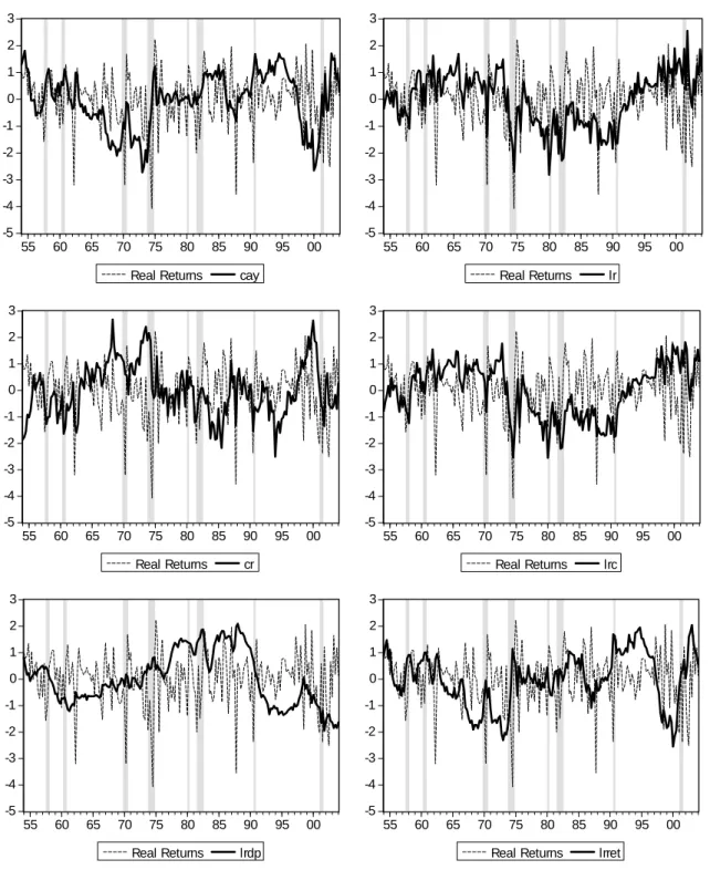
(12) 3. Expected Changes, Unexpected Shocks and Asset Returns. 3.1. Data In the estimations, I use quarterly, seasonally adjusted data for U.S., variables are measured at. 2000 prices and expressed in the logarithmic form of per capita terms, and the sample period is 1954:1 - 2004:1. The main data sources are the Flow of Funds Accounts provided by Board of Governors of Federal Reserve System and Bureau of Economic Analysis of U.S. Department of Commerce. In Appendix A, I present a detailed discussion of data. The de…nition of consumption includes nondurable consumption goods and services. Data on income includes only labor income. The de…nition of total wealth corresponds to net worth of households and nonpro…t organizations, this is, the sum of housing wealth and …nancial wealth. Housing wealth (or home equity) is de…ned as the value of real estate held by households minus home mortgages. Original data on wealth correspond to the end-period values. Therefore, I lag once the data, so that the observation of wealth in t corresponds to the value at the beginning of the period t + 1. Finally, asset returns are measured using the value weighted CRSP (CRSP-VW) market return index. ^. ^. ^. ^. ^. ^. Figure 1 plots the time series of cayt , lrt , crt , lrct , lrdpt , lrrett (based on the expected forecasts generated by the VAR) and the stock market real return, rt .15 It shows a multitude of episodes during which sharp increases in these proxies precede large reductions in the real return and it displays ^. ^. interesting business cycle patterns: (i) cayt and lrct increase during recessions and fall during expan^. ^. sions; and (ii) lrt and crt decrease during recessions and increase during expansions. It also shows ^. that lrdpt does not seem to be a good predictor of future returns, and this may be the result of its ^. high persistence Finally, the pattern of lrrett , this is, the proxy for the ex-ante expected long-run returns captures captures relatively well the pattern of the ex-post returns, which suggests that, for small perturbations around the steady state, the variables included in the VAR should capture most of the relevant information for the asset returns.. 1 5 Real. returns are constructed as the di¤erence between the CRSP-VW market return index and the in‡ation rate.. The time series are standardized to have unit variance and smoothed to facilitate the reading.. 10.

(13) Figure 1: Time series of cay, lr, cr, lrc, lrdp, lrret and real returns. All series are norm alized to standard deviations. The sam ple p eriod is 1954:1 to 2004:1. Shaded areas denote NBER recessions.. 3. 3. 2. 2. 1. 1. 0. 0. -1. -1. -2. -2. -3. -3. -4. -4. -5. -5 55. 60. 65. 70. 75. 80. 85. Real Returns. 90. 95. 00. 55. 60. 65. 70. cay. 75. 80. 85. Real Returns. 3. 3. 2. 2. 1. 1. 0. 0. -1. -1. -2. -2. -3. -3. -4. -4. -5. 90. 95. 00. 95. 00. 95. 00. lr. -5 55. 60. 65. 70. 75. 80. 85. Real Returns. 90. 95. 00. 55. 60. 65. 70. cr. 75. 80. 85. Real Returns. 3. 3. 2. 2. 1. 1. 0. 0. -1. -1. -2. -2. -3. -3. -4. -4. -5. 90 lrc. -5 55. 60. 65. 70. 75. 80. Real Returns. 85. 90. 95. 00. 55. lrdp. 60. 65. 70. 75. 80. Real Returns. 11. 85. 90 lrret.

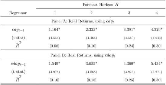
(14) 3.2. Consumption-Wealth Ratio ^. ^. ^. ^. ^. ^. I examine the relative predictive power of cayt ; lrt ; crt ; lrct ; lrdpt ; lrrett for real returns over horizons spanning 1 to 4 quarters. In the estimation of the regressions of real returns, the dependent variable is the H-period log real return on the CRSP-VW Index, rt+1 + :: + rt+H . For each regression - with the exceptions of cay and cday in Table 1 -, the tables report the estimates from OLS regressions based on the expected long-run forecasts (Panel A) and on the unexpected long-run deviations (Panel B) and all equations include lag returns as a regressor. Lettau and Ludvigson (2001) show that ‡uctuations in the consumption-aggregate wealth ratio, cay, summarize changes in expected returns and can be used for predicting stock returns. Investors want to maintain a ‡at consumption path over time and will attempt to "smooth out" transitory movements in their asset wealth arising from time variation in asset returns. When excess returns are, for example, expected to be higher in the future, forward-looking investors will react by increasing consumption out of current asset wealth and labor income, allowing consumption to rise above its common trend with those variables. More recently, Sousa (2006) shows that ‡uctuations in the consumption-(dis)aggregate wealth ratio, cday, have superior forecasting power due to its ability to track the changes in the composition of asset wealth (…nancial versus housing wealth) and the faster rate of convergence of the coe¢ cients to the "long-run equilibrium" parameters. I analyze the forecasting power of cay and cday for real returns. I estimate cay as cayt := ct 0:42wt. 0:65yt and cday as cdayt := ct. 0:29ft. 0:17ut. 0:60yt , where ct , yt , wt , ft and ut represent,. respectively, nondurable consumption of goods and services, labor income, aggregate asset wealth, …nancial wealth and housing wealth.16 ^. Table 1 reports a summary of the results. Panel A shows that cay has a signi…cant forecasting power _2. for future real returns, particularly at 3 and 4 quarters horizons, with the R statistic reaching 0.30, consistent with Lettau and Ludvigson (2001). In accordance with Sousa (2006), Panel B shows that ^. cday performs better: the coe¢ cient estimates are larger in magnitude and, for the same horizons, the _2. R statistic ranges between 0.25 and 0.30. This suggests that the disaggregation of wealth into its main components is an important issue in the context of forecasting future asset returns.17 16 I. estimate cayt and cdayt using dynamic OLS with 4 lags and leads.. 1 7 The. ^. ^. predictive impact of cday on future returns is economically larger than that of cay: in the one-period ahead ^. ^. regressions, the point estimate of the coe¢ cient on cday is about 1.549 for real returns and only 1.164 in the case of cay. ^. Thus, a one-standard-deviation increase in cday (standard deviation is 0.019) leads to, approximately, a 82.07 basis points rise in the expected real return on value weighted CRSP index, this is, a 3.32% increase at an annual rate. On the other ^. ^. hand, cay itself has a standard deviation of about 0.023, implying that a one-standard-deviation increase in cay leads to, approximately, a 50 basis points rise in the expected real return on value weighted CRSP index, this is, a 2.02% increase. 12.

(15) Table 1: Forecasting real Returns using cay and cday. Forecast Horizon H Regressor. 1. 2. 3. 4. ^. Panel A: Real Returns, using cayt. cayt. 1. 1.164*. 2.325*. 3.381*. 4.329*. (t-stat). (4.554). (4.466). (4.560). (4.944). [0.08]. [0.16]. [0.24]. [0.30]. _2. R. ^. Panel B: Real Returns, using cdayt. cdayt. 1. 1.549*. 3.055*. 4.360*. 5.434*. (t-stat). (4.978). (4.868). (4.975). (5.271). [0.10]. [0.18]. [0.25]. [0.30]. _2. R. Symbols *, ** and *** represent signi…cance at a 1%, 5% and 10% level, respectively. Newey-West (1987) corrected t-statistics appear in parenthesis. The sample period is 1954:1 to 2004:1.. 3.3. Long-Run Changes in the Composition of Consumption In the standard model, investors’ concern with consumption risk implies that stock prices move. with the business cycle. In recessions, investors expect higher future consumption and try to sell stocks today to increase current consumption. This intertemporal substitution mechanism drives down stock prices in bad times. Yogo (2006) shows that when utility is nonseparable in nondurable and durable consumption and the elasticity of substitution between the two consumption goods is su¢ ciently high, marginal utility rises when durable consumption falls.18 Stock returns are unexpectedly low at business cycle troughs, when durable consumption falls sharply, and this helps to explain the countercyclical variation in the equity premium. Piazzesi et al. (2007) consider a consumption-based asset pricing model where housing is explicitly modelled both as an asset and as a consumption good. Nonseparable preferences describe households’ concern with composition risk, that is, ‡uctuations of the relative share of non-housing in their consumption basket and the model predicts that the housing share can be used to forecast returns on stocks. Finally, Lustig and Van Nieuwerburgh (2005) show that in a model with housing collateral, the ratio of housing wealth to human wealth shifts the conditional distribution of asset prices at an annual rate. 1 8 Dunn and Singleton (1986) and Eichenbaum and Hansen (1990) report evidence against separabilility of preferences, but they conclude that introducing durables does not help in reducing the pricing errors for stocks.. 13.

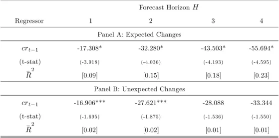
(16) and consumption growth and, therefore, predicts returns on stocks. The authors consider two main channels that transmit shocks originated in the housing market to the risk premia in asset market: (i) when housing prices decrease, collateral is destroyed and households are more exposed to idiosyncratic labor income risk; and (ii) households want to hedge against rental price shocks or consumption basket composition shocks when the utility function is nonseparable in nondurable consumption and housing services. I analyze the forecasting power of housing share for asset returns. However, instead of imposing nonseparability of preferences, as in the works mentioned above, I use the intertemporal budget constraint to derive a relationship between the present discount value of changes in housing share, cr, and asset returns. Moreover, while the focus of previous literature is on the forecasting power of housing share, I focus instead in the long-run changes of the housing share Finally, with the VAR estimated in Section 2.2, I estimate and compare the forecasting power of expected and unexpected changes in housing share. Table 2 presents a summary of the results. Panel A shows that expected changes in the housing share _2. strongly forecast future real returns, with the R statistic ranging from 0.09 to 0.23. In contrast, Panel _2. B shows that unexpected growth has only a small predictive power (the R statistic ranges between 0.01 and 0.02). In both regressions, the coe¢ cient associated to cr is negative, consistent with the fact that a high cr represents a state of the world in which returns on asset wealth are low. This suggests that while expected changes in the long-run housing share are an important determinant of real returns, unexpected changes do not play an important role in the context of forecasting asset returns, contradicting the results obtained in Lustig and Van Nieuwerburgh (2005) and Piazzesi et al. (2007). The reason lies in the observation that housing share is a macroeconomic variable with a high degree of persistent and, therefore, its changes can largely be forecasted by consumers. As a result, long-run composition risk plays a negligible role in forecasting asset returns.. 14.

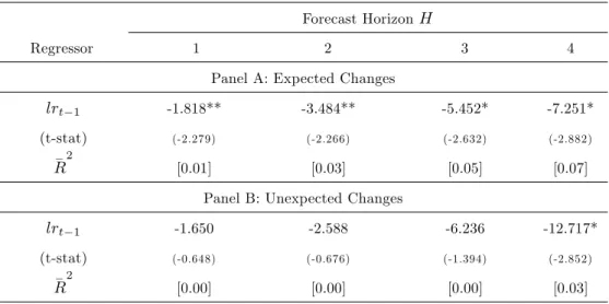
(17) Table 2: Forecasting real returns using cr. Forecast Horizon H Regressor. 1. 2. 3. 4. Panel A: Expected Changes. crt. 1. (t-stat). -17.308*. -32.280*. -43.503*. -55.694*. (-3.918). (-4.036). (-4.193). (-4.595). [0.09]. [0.15]. [0.18]. [0.23]. _2. R. Panel B: Unexpected Changes. crt. 1. (t-stat). -16.906***. -27.621***. -28.088. -33.344. (-1.695). (-1.875). (-1.536). (-1.550). [0.02]. [0.02]. [0.01]. [0.01]. _2. R. Symbols *, ** and *** represent signi…cance at a 1%, 5% and 10% level, respectively. Newey-West (1987) corrected t-statistics appear in parenthesis. The sample period is 1954:1 to 2004:1.. 3.4. Long-Run Labor Income Growth Julliard (2004) uses the representative consumer’s budget constraint to derive an equilibrium rela-. tion between expected future labor income growth rates - summarized by the variable lr - and expected future asset returns. The author shows that expectations of high (low) future labor income growth are associated with lower (higher) stock market excess returns. These results are consistent with the fact that high lr represents a state of the world in which agents expect to have abundance of resources in the future to …nance consumption, therefore low returns on asset wealth are feared less and lower equilibrium risk premia are required. In order to model the labor income process, the author experimented with several speci…cations in the ARIMA class, and performed the standard set of Box-Jenkins selection procedures.19 In the present paper, I use a di¤erent methodology in that expected and unexpected labor income growth rates are computed directly from the VAR estimated in Section 2.2. Table 3 presents a summary of the results describing the forecasting power of lr: Panel A considers the expected long-run growth as the major explanatory variable, while Panel B includes only the unexpected long-run shocks. In both regressions, the coe¢ cient associated to lr is negative, consistent with the fact that a high lr represents a state of the world in which returns on asset wealth are low. Moreover, it can be seen that, consistently with Julliard (2004), expected growth has a signi…cant 1 9 In. particular, the ARIMA(0,1,2) speci…cation for log income …ts well the data.. 15.

(18) _2. forecasting power for future real returns, with the R statistic ranging from 0.01 to 0.07. In contrast, Panel B shows that unexpected growth has no predictive power. In sum, long-run labor income growth is an important determinant of real returns, while unexpected changes do not play an important role in the context of forecasting asset returns. Table 3: Forecasting real returns using lr. Forecast Horizon H Regressor. 1. 2. 3. 4. Panel A: Expected Changes. lrt. 1. (t-stat). -1.818**. -3.484**. -5.452*. -7.251*. (-2.279). (-2.266). (-2.632). (-2.882). [0.01]. [0.03]. [0.05]. [0.07]. _2. R. Panel B: Unexpected Changes. lrt. 1. (t-stat). -1.650. -2.588. -6.236. -12.717*. (-0.648). (-0.676). (-1.394). (-2.852). [0.00]. [0.00]. [0.00]. [0.03]. _2. R. Symbols *, ** and *** represent signi…cance at a 1%, 5% and 10% level, respectively. Newey-West (1987) corrected t-statistics appear in parenthesis. The sample period is 1954:1 to 2004:1.. 3.5. Long-Run Consumption Growth Bansal et al. (2005) show that asset prices re‡ect the discounted value of cash ‡ows and that. return news re‡ect revisions in expectations about the entire path of future cash ‡ows and discount rates. Changes in expectations of cash ‡ows is an important ingredient determining asset return news. Systematic risks in cash ‡ows therefore should have some bearing on the risk compensation of assets. In particular, assets whose cash ‡ows have higher aggregate consumption risks should also carry a higher risk premium. This intuition is also captured in the consumption-based models presented in Abel (1999) and Bansal and Yaron (2004), who show that di¤erences in risk compensation on assets mirror di¤erences in the exposure of assets’cash ‡ows to consumption. Economic risks in cash ‡ows, an important ingredient determining asset returns, provide very valuable information about systematic risks in asset returns. By its turn, Parker and Julliard (2005) study the Fama and French size and book-to-market portfolios and reevaluate the central insight of the consumption capital asset pricing model that an asset’s expected 16.

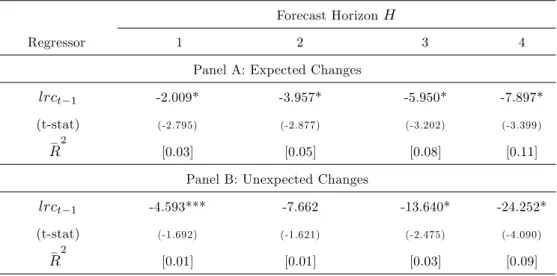
(19) return is determined by its equilibrium risk to consumption. Rather than measure the risk of a portfolio by the contemporaneous covariance of its return and consumption growth, the authors measure the risk of a portfolio by its ultimate risk to consumption, de…ned as the covariance of its return and consumption growth over the quarter of the return and many following quarters. This paper is based on a similar argument: instead of looking at the forecasting power of current consumption’s growth for asset returns, the focus is on the long-run consumption growth, lrc. Using the VAR estimated in Section 2.2, I compute the expected and the unexpected long-run consumption growth and then use them as explanatory variables for one-period ahead real returns. Table 4 presents a summary of the results: Panel A includes the expected changes as the major explanatory variable, while Panel B includes the unexpected changes. It can be seen that the coe¢ cient associated to lrc is negative in both regressions, consistent with the fact that a high lrc represents a state of the world in which returns on asset wealth are low. This also implies that consumers try to hedge future ‡uctuations in consumption by investing in the stock markets, that is, stocks are used as an hedging device against negative future consumption shocks. The results are, therefore, in line with the …ndings of Parker and Julliard (2005). Table 4: Forecasting real returns using lrc. Forecast Horizon H Regressor. 1. 2. 3. 4. Panel A: Expected Changes. lrct. 1. -2.009*. -3.957*. -5.950*. -7.897*. (t-stat). (-2.795). (-2.877). (-3.202). (-3.399). [0.03]. [0.05]. [0.08]. [0.11]. _2. R. Panel B: Unexpected Changes. lrct. 1. (t-stat). -4.593***. -7.662. -13.640*. -24.252*. (-1.692). (-1.621). (-2.475). (-4.090). [0.01]. [0.01]. [0.03]. [0.09]. _2. R. Symbols *, ** and *** represent signi…cance at a 1%, 5% and 10% level, respectively. Newey-West (1987)] corrected t-statistics appear in parenthesis. The sample period is 1954:1 to 2004:1.. 17.

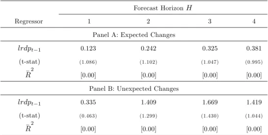
(20) 3.6. Long-Run Dividend-Price Ratio Shiller (1984), Campbell and Shiller (1998), and Fama and French (1988) all …nd that the ratios of. price to dividends or earnings have predictive power for excess returns. Lamont (1998) …nds that the ratio of dividend to earnings has forecasting power at quarterly horizons. Campbell (1991) and Hodrick (1992) …nd that the relative T-bill rate (the 30-day T-bill rate minus its 12-month moving average) predicts returns, and Fama and French (1989) study the forecasting power of the term spread (the 10year Treasury bond yield minus the 1-year Treasury bond yield) and the default spread (the di¤erence between the BAA and AAA corporate bond rates). Lamont (1998) argues that the dividend payout ratio should be a potentially potent predictor of excess returns, a result of the fact that high dividends typically forecast high returns whereas high earnings typically forecast low returns. On the other hand, Lettau and Ludvigson (2001a) show that these predictors do not convey signi…cant information about future asset returns. I use the VAR estimated in Section 2.2 to build measures of the long-run dividend-price ratio, lrdp, and test its forecasting power over di¤erent horizon spans. Table 5 presents a summary of the results and shows that the long-run dividend to price ratio does not contain explanatory power for real returns in accordance with the …ndings of Lettau and Ludvigson (2001a). Empirically, this result can be explained by the poor dynamics (and huge persistence) of lrdp, which does not enable it to match the ‡uctuations that characterize asset returns. Table 5: Forecasting real returns using lrdp. Forecast Horizon H Regressor. 1. 2. 3. 4. Panel A: Expected Changes. lrdpt. 1. 0.123. 0.242. 0.325. 0.381. (t-stat). (1.086). (1.102). (1.047). (0.995). [0.00]. [0.00]. [0.00]. [0.00]. _2. R. Panel B: Unexpected Changes. lrdpt. 1. 0.335. 1.409. 1.669. 1.419. (t-stat). (0.463). (1.299). (1.430). (1.044). [0.00]. [0.00]. [0.00]. [0.00]. _2. R. Symbols *, ** and *** represent signi…cance at a 1%, 5% and 10% level, respectively. Newey-West (1987) corrected t-statistics appear in parenthesis. The sample period is 1954:1 to 2004:1.. 18.

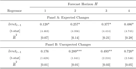
(21) 3.7. Long-Run Asset Returns Most of the literature on asset pricing aimed at building proxies of asset returns measure the fore-. casting power relating these proxies with ex-post realized asset returns. Favero (2005) tries to highlight the di¤erences between ex-ante expected returns and ex-post realized returns. The author derives a proxy for the long-run expected returns using a VAR that includes asset returns, cay, consumption growth and asset returns. After realization, the VAR is re-estimated each point in time and projected forward for a long-horizon, so that long-run expected returns are computed. I compute a proxy for the expected and unexpected long-run asset returns, lrret, using the VAR estimated in Section 2.2. While the focus of Favero (2005) is on assessing the di¤erences between these and the predictive power of cay, I aim at analyzing to which extent asset returns re‡ect expectations about future returns and the importance of unexpected shocks. Table 6 presents a summary of the results. Panel A shows that expected ex-ante changes in long-run _2. real returns strongly forecast future real returns, with the R statistic ranging from 0.07 to 0.28. Panel B shows that unexpected ex-ante changes in long-run real returns also have some predictive power (the _2. R statistic ranges between 0.01 and 0.05). This suggests that both expected and unexpected changes in the ex-ante long-run asset returns are important determinants of real returns. This means that expectations about future returns represent only a small component of the behaviour of observed asset returns and that other forces drive this variable. Table 6: Long-run horizon regressions using lrret. Forecast Horizon H Regressor. 1. 2. 3. 4. Panel A: Expected Changes. lrrett. 1. (t-stat]. 0.128*. 0.257*. 0.377*. 0.486*. (4.463). (4.356). (4.414). (4.745). [0.07]. [0.14]. [0.21]. [0.28]. _2. R. Panel B: Unexpected Changes. lrrett. 1. (t-stat]. 0.176. 0.289***. 0.493**. 0.720*. (1.628). (1.841). (2.218). (2.546). [0.01]. [0.01]. [0.03]. [0.05]. _2. R. Symbols *, ** and *** represent signi…cance at a 1%, 5% and 10% level, respectively. Newey-West (1987) corrected t-statistics appear in parenthesis. The sample period is 1954:1 to 2004:1.. 19.

(22) 4. Conclusion This paper uses the representative consumer’s budget constraint to derive an equilibrium relation. between the trend deviations among consumption, aggregate wealth and labor income, cay, expected future changes in the housing consumption share, cr, expected future labor income growth, lr, expected future consumption growth, lrc, and expected future asset returns, and explores the predictive power of these variables for future asset returns. The novelty of the paper is in the methodology. Instead of relying on a model of consumer behaviour that explicitly assumes a functional form for preferences, I use the intertemporal budget constraint to derive the major determinants of asset returns. Then, I explore the forecasting properties of an informative VAR to build proxies for the long-run determinants of asset returns. Finally, the forecasting power of these proxies for future asset returns is assessed and this is used as a way of indirectly testing the assumptions about preferences considered in many optimal models of consumer behaviour. Using a Vector Autoregressive System (VAR), I compute measures of expected and unexpected longrun changes of the major determinants of asset returns and …nd that: (i) cay, cday, expected future labor income growth, expected future changes in the composition of consumption, expected future consumption growth, expected changes in ex-ante long-run real returns strongly forecast future asset returns; (ii) unexpected long-run consumption growth and unexpected changes in ex-ante long-run real returns contain some predictive power for asset returns; (iii) unexpected future labor income growth and unexpected changes in the housing share do not predict future asset returns; and (iv) neither expected nor unexpected changes in the dividend price-dividend ratio forecast asset returns. Moreover, this work suggests that agents’expectations about long-run risk are important and that asset returns largely re‡ect that information. The results show that expectations of high future labor income, expectations of high future consumption growth, and expectations of high non-housing consumption share are associated with lower stock market returns, and low labor income growth expectations, low consumption growth expectations and low non-housing consumption share expectations are associated with higher than average real returns. Therefore, the success of lr, cr, and lrc as predictors of asset returns seems to be due to their ability to track risk premia. On the other hand, shocks to long-run expectations seem to play a negligible role as their forecasting power for current returns is, in general, very low.. 20.

(23) References ABEL, A. (1999), "Risk premia and term premia in general equilibrium", Journal of Monetary Economics, 43, 3-33. ATTANASIO, O.; DAVIS, S. J. (1996), “Relative wage movements and the distribution of consumption”, Journal of Political Economy, 104(6), 1227-1262. ATTANASIO, O.; WEBBER, G. (1995), "Is consumption growth consistent with intertemporal optimization? Evidence from the Consumer Expenditure Survey”, Journal of Political Economy, 103(6), 1121-57. BANSAL, R.; YARON, A. (2004), "Risks for the long run: a potential resolution of asset pricing puzzles", Journal of Finance, 59(4), 1481-1509. BANSAL, R.; DITTMAR, R. F.; LUNDBLAD, C. T. (2005), "Consumption, dividends, and the cross section of equity returns", Journal of Finance, 60(4), 1639-1672. BASU, S.; KIMBALL, M. S. (2000), “Long-run labor supply and the elasticity of intertemporal substitution for consumption”, University of Michigan manuscript. BAXTER, M.; JERMANN, U. J. (1999), "Household production and the excess sensitivity of consumption to current income”, American Economic Review, 89, 902-20. BAXTER, M.; JERMANN, U. J. (1997), “The international diversi…cation puzzle is worse than you think”, American Economic Review, 87, 170-180. BRAINARD, W. C.; NELSON, W. R.; SHAPIRO, M. D. (1991), “The consumption beta explains expected returns at long horizons”, Yale University manuscript. BREEDEN, D. T. (1979), “An intertemporal asset pricing model with stochastic consumption and investment opportunities”, Journal of Financial Economics, 7, 265-296. BREEDEN, D. T.; GIBBONS, M. R.; LITZENBERGER, R. H. (1989), "Empirical tests of the consumption-oriented CAPM”, Journal of Finance, 44, 231–62. CAMPBELL, J. Y. (1991), "A variance decomposition for stock returns", Economic Journal, 101, 157-179.. 21.

(24) CAMPBELL, J. Y. (1996), “Understanding risk and return", Journal of Political Economy, 104, 298– 345. CAMPBELL, J.; COCHRANE, J. (1999), "By force of habit: a consumption-based explanation of aggregate stock market behavior", Journal of Political Economy, 107, 205-251. CAMPBELL, J. Y.; DEATON, A. (1989), “Why is consumption so smooth?”, Review of Economic Studies, 56 (3), 357-373. CAMPBELL, J.; MANKIW, N. (1989), "Consumption, income, and interest rates: reinterpreting the time series evidence" in BLANCHARD, O.; FISCHER, S., eds., NBER Macroeconomics Annual, MIT Press, Cambridge, Massachussets, 185-216. CAMPBELL, J. Y.; SHILLER, R. J. (1987), “Cointegration and tests of present value models”, Journal of Political Economy, 95, 1062-1088. CAMPBELL, J. Y.; SHILLER, R. J. (1988), "The dividend-price ratio and expectations of future dividends and discount factors", Review of Financial Studies, 1(3), 195-228. CARROLL, C. D. (1997), “Bu¤er stock saving and the life cycle/permanent income hypothesis”, Quarterly Journal of Economics, 112(1), 1-55. COCHRANE, J. H. (1996), “A cross-sectional test of an investment-based asset pricing model”, Journal of Political Economy, 104, 572–621. COCHRANE, J. H. (1991), “A simple test of consumption insurance”, Journal of Political Economy, 99(5), 957-976. CONSTANTINIDES, G. (1990), "Habit-formation: a resolution of the equity premium puzzle", Journal of Political Economy, 98, 519-543. DUNN, K.; SINGLETON, K. (1986), “Modelling the term structure of interest rates under nonseparable utility and durability of goods”, Journal of Financial Economics, 17(1), 27-55. EICHENBAUM, M.; HANSEN, L. P. (1990), "Estimating models with intertemporal substitution using aggregate time series data", Journal of Business and Economic Statistics, 8(1), 53-69. FAMA, E. F., FRENCH, K. R. (1988), “Permanent and temporary components of stock prices”, Journal of Political Economy, 96, 246-273.. 22.

(25) FAMA, E. F.; FRENCH, K. R. (1992), “The cross-section of expected stock returns”, Journal of Finance, 47, 427-465. FAVERO, C. (2005), "Consumption, wealth, the elasticity of intertemporal substitution and long-run stock market returns", Bocconi University, manuscript. FERNANDEZ-CORUGEDO, E.; PRICE, S.; BLAKE, A. (2003), "The dynamics of consumers’ expenditure: the UK consumption ECM redux", Bank of England Working Paper #204. FLAVIN, M. (1981), “The adjustment of consumption to changing expectations about future income", Journal of Political Economy, 89, 974-1009. GOURINCHAS, P.-O. (2000), “Precautionary saving, life cycle and macroeconomics”, Princeton University manuscript. HANSEN, L. P.; SINGLETON, K. J. (1982), “Generalized instrumental variables estimation of nonlinear rational expectations models”, Econometrica, 50, 1269-1286. HALL, R. E. (1988), “Intertemporal substitution in consumption”, Journal of Political Economy, 96(2), 339-357. HODRICK, R. J. (1992), "Dividend yields and expected stock returns: alternative procedures for inference and measurement", Review of Financial Studies, 5(3), 357-386. JAGANNATHAN, R.; WANG, Z. (1996), "The conditional CAPM and the cross-section of expected returns", Journal of Finance, 51, 3-54. JULLIARD, C. (2004), "Labor income risk and asset returns", Princeton University, Primary Job Market Paper. KRUSELL, P.; SMITH, A. A. (1998), “Income and wealth heterogeneity in the macroeconomy”, Journal of Political Economy, 106(5), 867-896. LETTAU, M.; LUDVIGSON, S. (2001a), “Consumption, aggregate wealth, and expected stock returns”, Journal of Finance, 56(3), 815-849. LETTAU, M.; LUDVIGSON, S. (2001b), “Resurrecting the (C)CAPM: a cross-sectional test when risk premia are time-varying”, Journal of Political Economy, 109, 1238-1286. LETTAU, M.; LUDVIGSON, S. (2004), "Understanding trend and cycle in asset values: reevaluating the wealth e¤ect on consumption", American Economic Review, 94(1), 276-299. 23.

(26) LINTNER, J. (1965), "The valuation of risky assets and the selection of risky investments in stock portfolios and capital budgets", Review of Economics and Statistics, 47, 13–37. LUCAS, R. E. (1978), “Asset prices in an exchange economy”, Econometrica, 46, 1429-1445. LUSTIG, H.; VAN NIEUWERBURGH, S. (2005), "Housing collateral, consumption insurance, and risk premia: an empirical perspective", Journal of Finance, 60(3), 1167-1219. MANKIW, N. G.; SHAPIRO, M. D. (1986), “Risk and return: consumption beta versus market beta”, Review of Economics and Statistics, 68, 452-59. NELSON, J. A. (1994), “On testing for full insurance using Consumer Expenditure Survey data”, Journal of Political Economy, 102 (2), 384-94. OGAKI, M.; REINHART, C. M. (1998), "Measuring intertemporal substitution: the role of durable goods”, Journal of Political Economy, 106 (5), 1078-1098. PAKOS, M. (2003), "Asset pricing with durable goods and non-homothetic preferences", University of Chicago, manuscript. PARKER, J. A.; JULLIARD, C. (2005), "Consumption risk and the cross section of expected returns", Journal of Political Economy, 113(1), 185-222. PARKER, J. A.; PRESTON, B. (2005), "Precautionary saving and consumption ‡uctuations", American Economic Review, 95(4), 1119-1143. PIAZZESI, M.; SCHNEIDER, M.; TUZEL, S. (2007), "Housing, consumption and asset pricing", Journal of Financial Economics, 83, 531-569. POTERBA, J.; SUMMERS, L. (1988), “Mean reversion in stock prices: evidence and implications”, Journal of Financial Economics, 22, 27-60. RICHARDS, A. (1995), "Comovements in national stock market returns: evidence of predictability, but not cointegration", Journal of Monetary Economics, 36, 631-654. RIOS-RULL, V. (1994), “On the quantitative importance of market completeness”, Journal of Monetary Economics, 34, 462-496. SHARPE, W. (1964), "Capital asset prices: a theory of market equilibrium under conditions of risk", Journal of Finance, 19, 425–442.. 24.

(27) SHILLER, R. J. (1982), “Consumption, asset markets, and macroeconomic ‡uctuations”, Carnegie Mellon Conference Series on Public Policy, 17, 203-238. SHILLER, R. J. (1984), “Stock prices and social dynamics”, Brookings Papers on Economic Activity, 84(2), 457-510. SOUSA, R. (2006), "Consumption, (dis)aggregate wealth, and asset returns", London School of Economics, manuscript. SUMMERS, L. H. (1986), “Does the stock market rationally re‡ect fundamental values?”, Journal of Finance, 41, 591-601. SUNDARESAN, S. (1989), "Intertemporally dependent preferences and the volatility of consumption and wealth", Review of Financial Studies, 2, 73-89. WEI, M. (2005), "Human capital, business cycles and asset pricing", Board of Governors of the Federal Reserve - Division of Monetary A¤airs, working paper. YOGO, M. (2006), "A consumption-based explanation of expected stock returns", Journal of Finance, 61(2), 539-580.. 25.

(28) Appendix A. Data Description. Consumption Consumption is de…ned as the expenditure in non-durable consumption goods and services. Data are quarterly, seasonally adjusted at an annual rate, measured in billions of dollars (2000 prices), in per capita terms and expressed in the logarithmic form. Series comprises the period 1947:1-2005:4. The source is U.S. Department of Commerce, Bureau of Economic Analysis, NIPA Table 2.3.5. Aggregate Wealth Aggregate wealth is de…ned as the net worth of households and nonpro…t organizations. Data are quarterly, seasonally adjusted at an annual rate, measured in billions of dollars (2000 prices), in per capita terms and expressed in the logarithmic form. Series comprises the period 1952:2-2006:1. The source of information is Board of Governors of Federal Reserve System, Flow of Funds Accounts, Table B.100, line 41 (series FL152090005.Q). After-Tax Labor Income After-tax labor income is de…ned as the sum of wage and salary disbursements (line 3), personal current transfer receipts (line 16) and employer contributions for employee pension and insurance funds (line 7) minus personal contributions for government social insurance (line 24), employer contributions for government social insurance (line 8 ) and taxes. Taxes are de…ned as: [(wage and salary disbursements (line 3)] / (wage and salary disbursements (line 3)+ proprietor’income with inventory valuation and capital consumption adjustments (line 9) + rental income of persons with capital consumption adjustment (line 12) + personal dividend income (line 15) + personal interest income (line 14))] * (personal current taxes (line 25)]. Data are quarterly, seasonally adjusted at annual rates, measured in billions of dollars (2000 prices), in per capita terms and expressed in the logarithmic form. Series comprises the period 1947:1-2005:4. The source of information is U.S. Department of Commerce, Bureau of Economic Analysis, NIPA Table 2.1.. Asset Returns The proxy chosen for the market return is the value weighted CRSP (CRSP-VW) market return index. The CRSP index includes NYSE, AMEX and NASDAQ, and should provide a better proxy 26.

(29) for market returns than the Standard & Poor (S&P) index since it is a much broader measure. Data are quarterly, de‡ated by the personal consumption chain-weighted index (2000=100) and expressed in the logarithmic form. Series comprises the period 1947:2-2004:4. The source of information is Robert Shiller’s web site: http://www.econ.yale.edu/~shiller/data.htm. Population Population was de…ned by dividing aggregate real disposable income (line 35) by per capita disposable income (line 37). Data are quarterly. Series comprises the period 1946:1-2001:4. The source of information is U.S. Department of Commerce, Bureau of Economic Analysis, NIPA Table 2.1. Price De‡ator The nominal wealth, after-tax income, consumption, and interest rates were de‡ated by the personal consumption expenditure chain-type price de‡ator (2000=100), seasonally adjusted. Data are quarterly. Series comprises the period 1947:1-2005:4. The source of information is U.S. Department of Commerce, Bureau of Economic Analysis, NIPA Table 2.3.4., line 1. In‡ation Rate In‡ation rate was computed from price de‡ator. Data are quarterly. Series comprises the period 1947:2-2005:4. The source of information is U.S. Department of Commerce, Bureau of Economic Analysis, NIPA Table 2.3.4, line 1. Interest Rate ("Risk-Free Rate") Risk-free rate is de…ned as the 3-month U.S. Treasury bills real interest rate. Original data are monthly and are converted to a quarterly frequency by computing the simple arithmetic average of three consecutive months. Additionally, real interest rates are computed as the di¤erence between nominal interest rates and the in‡ation rate. The 3-month U.S. Treasury bills real interest rate’series comprises the period 1947:2-2005:4, and the source of information is the H.15 publication of the Board of Governors of the Federal Reserve System.. 27.

(30) B. Vector-Autoregression (VAR) Estimation Table B1: Estimates from vector-autoregressions (VAR). Equation Dependent variable. st. 1. wt. 1. ct. 1. yt. rt. 1. 1. cayt. dt. 1. pt. 1. 1. st. wt. ct. yt. rt. cayt. dt. pt. 0.443*. -1.886*. -0.670**. -0.916. -8.303. 0.717. 0.039. (5.889). (-2.818). (-2.319). (-1.474). (-1.376). (1.422). (0.660). -0.000. -0.019. -0.009. -0.038. 0.146. 0.024. 0.002. (-0.063). (-0.556). (-0.585). (-1.192). (0.477). (0.929). (0.577). -0.059*. 0.585*. 0.280*. 0.583*. 1.138. -0.345**. 0.002. (-2.712). (3.010). (3.329). (3.228). (0.649). (-2.355). (0.130). 0.017***. 0.132. 0.080**. -0.111. -0.577. 0.096. 0.006. (1.799). (1.580). (2.213). (-1.428). (-0.766). (1.532). (0.822). 0.001. 0.212*. 0.011*. 0.020*. -0.045. -0.091*. 0.001. (1.002). (25.924). (3.247). (2.666). (-0.606). (-14.743). (1.284). -0.007***. -0.036. -0.026***. -0.024. 1.153*. 1.004*. -0.008*. (-1.830). (-1.137). (-1.930). (-0.821). (4.040). (42.182). (-2.982). -0.003. 0.055**. -0.075*. -0.048***. -0.667*. -0.067*. 1.005*. (-1.034). (1.955). (-6.199). (-1.853). (-2.631). (-3.165). (408.095). [0.16]. [0.80]. [0.20]. [0.08]. [0.07]. [0.91]. [0.91]. _2. R. This table reports the estimated coe¢ cients from vector-autoregressions (VAR). Symbols *, **, *** represent, respectively, signi…cance level of 1%, 5% and 10%. Newey-West (1987) corrected t-statistics appear in parenthesis. The sample period is 1953:4 to 2004:4.. 28.

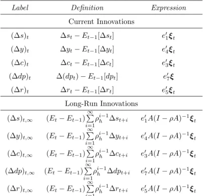
(31) C. Notation: Current and Long-Run Innovations Table C1: Notation - current and long-run innovations. Label. De…nition. Expression. Current Innovations ( s)t. st. Et. 1[. st ]. e01. t. ( y)t. yt. Et. 1[. yt ]. e04 t. ( c)t. ct. Et. 1[. ct ]. e03. 1 [dpt ]. e07. rt ]. e05. ( dp)t. (dpt ). ( r)t. rt. ( s)t;1. (Et. ( y)t;1. (Et. ( c)t;1. (Et. ( dp)t;1. (Et. ( r)t;1. (Et. Et Et. 1[. t. t. Long-Run Innovations 1 P i 1 Et 1 ) st+i e01 A(I h. A). 1. yt+i. e04 A(I. A). 1. ct+i. e03 A(I. A). 1. dpt+i. e07 A(I. A). 1. rt+i. e05 A(I. A). 1. i=1 1 P. i 1 1) h i=1 1 P i 1 Et 1 ) h i=1 1 P i 1 Et 1 ) h i=1 1 P i 1 Et 1 ) h i=1. Et. t t t t t. The subscript t denotes current innovations. The subscript t; 1 denotes current and future innovations.. 29.

(32) Most Recent Working Papers NIPE WP 28/2007. Sousa, Ricardo M., “Wealth Shocks and Risk Aversion”, 2007.. NIPE WP 27/2007. Esteves, Rosa Branca, “Pricing with Customer Recognition”, 2007.. NIPE WP 26/2007. Alexandre, Fernando, Pedro Bação and John Driffill, ”Optimal monetary policy with a regime-switching exchange rate in a forward-looking model”, 2007. Lommerud, Kjell Erik and Odd Rune Straume, “Technology resistance and globalisation with trade unions: the choice between employment protection and flexicurity”, 2007 Aidt, Toke S., Veiga, Francisco José, Veiga, Linda Gonçalves, “Election Results and Opportunistic Policies: An Integrated Approach”, 2007 Torres, Francisco, “The long road to EMU: The Economic and Political Reasoning behind Maastricht”, 2007. Torres, Francisco, “On the efficiency-legitimacy trade-off in EMU”, 2007.. NIPE WP 25/2007 NIPE WP 24/2007 NIPE WP 23/2007 NIPE WP 22/2007 NIPE WP 21/2007 NIPE WP 20/2007 NIPE WP 19/2007 NIPE WP 18/2007. Torres, Francisco, “A convergência para a União Económica e Monetária: objectivo nacional ou constrangimento externo?”, 2007. Bongardt, Annette and Francisco Torres, “Is the ‘European Model’ viable in a globalized world?”, 2007. Bongardt, Annette and Francisco Torres, “Institutions, Governance and Economic Growth in the EU: is there a role for the Lisbon Strategy?”, 2007. Monteiro, Natália and Miguel Portela, "Rent-sharing in Portuguese Banking", 2007.. NIPE WP 13/2007. Aguiar-Conraria, Luís Nuno Azevedo, and Maria Joana Soares, "Using Wavelets to Decompose the Time-Frequency Effects of Monetary Policy", 2007. Aguiar-Conraria, Luís and Maria Joana Soares, "Using cross-wavelets to decompose the time-frequency relation between oil and the macroeconomy", 2007. Gabriel, Vasco J., Alexandre, Fernando, Bação, Pedro, “The Consumption-Wealth Ratio Under Asymmetric Adjustment”, 2007. Sá, Carla; Florax, Raymond; Rietveld, Piet; “Living-arrangement and university decisions of Dutch young adults”, 2007. Castro, Vítor; “The Causes of Excessive Deficits in the European Union”, 2007.. NIPE WP 12/2007. Esteves, Rosa Branca; “Customer Poaching and Advertising”, 2007.. NIPE WP 17/2007 NIPE WP 16/2007 NIPE WP 15/2007 NIPE WP 14/2007. NIPE WP 11/2007 NIPE WP 9/2007 NIPE WP 8/2007 NIPE WP 7/2007 NIPE WP 6/2007 NIPE WP 5/2007 NIPE WP 4/2007 NIPE WP 3/2007 NIPE WP 2/2007. Portela, Miguel, Nelson Areal, Carla Sá, Fernando Alexandre, João Cerejeira, Ana Carvalho, Artur Rodrigues; “Regulation and marketisation in the Portuguese higher education system”, 2007. Brekke, Kurt R., Luigi Siciliani, Odd Rune Straume; “Competition and Waiting Times in Hospital Markets”, 2007. Thompson, Maria; “Complementarities and Costly Investment in a One-Sector Growth Model”, 2007. Monteiro, Natália; “Regulatory reform and labour earnings in Portuguese banking”, 2007. Magalhães, Manuela; “A Panel Analysis of the FDI Impact on International Trade”, 2007. Aguiar-Conraria, Luís; “A Note on the Stability Properties of Goodwin's PredatorPrey Model”, 2007. Cardoso, Ana Rute; Portela, Miguel; Sá, Carla; Alexandre, Fernando; “Demand for higher education programs: the impact of the Bologna process”, 2007. Aguiar-Conraria, Luís and Yi Wen, “Oil Dependence and Economic Instability, 2007. Cortinhas, Carlos, “Exchange Rate Pass-Through in ASEAN: Implications for the Prospects of Monetary Integration in the Region”, 2007..

(33)

No results found