World Wheat Price Volatility

(1)

Thompson, W., G. Smith and A. Elasri (2012), “World

Wheat Price Volatility: Selected Scenario Analyses”,

OECD

Food, Agriculture and Fisheries Papers

, No. 59, OECD

Publishing.

http://dx.doi.org/10.1787/5k8zpt62fs32-en

OECD Food, Agriculture and Fisheries

Papers No. 59

World Wheat Price Volatility

SELECTED SCENARIO ANALYSES

Wyatt Thompson, Garry Smith,

Armelle Elasri

(2)

AND FISHERIES PAPERS

The OECD Food, Agriculture and Fisheries Papers series is designed to make available to a wide readership selected studies by OECD staff or by outside consultants. This series continues that originally entitled OECD Food, Agriculture and Fisheries Working Papers.

This document and any map included herein are without prejudice to the status of or sovereignty over any territory, to the delimitation of international frontiers and boundaries and to the name of any territory, city or area.

This document has been declassified on the responsibility of the Working Party on

Agricultural Policies and Markets under OECD reference number

TAD/CA/APM/WP(2011)28/FINAL.

Comments on the series are welcome and should be sent to [email protected].

OECD FOOD, AGRICULTURE AND FISHERIES PAPERS

are published on

www.oecd.org/agriculture

You can copy, download or print OECD content for your own use, and you can include excerpts from OECD publications, databases and multimedia products in your own documents, presentations, blogs, websites and teaching materials, provided that suitable acknowledgment of OECD as source and copyright owner is given. All requests for commercial use and translation rights should be submitted to [email protected].

(3)

Abstract

WORLD WHEAT PRICE VOLATILITY:

SELECTED SCENARIO ANALYSES

Wyatt Thompson, University of Missouri, United States

Garry Smith and Armelle Elasri, OECD

This study provides quantitative assessments of the impact of two structural changes that have been identified as contributing to world wheat market price volatility. The factors examined in this paper relate to changes in demand in the BRICs (Brazil, Russian Federation, India and China) countries as a result of continuing economic growth and development, and the effects of lower levels of global wheat stocks in recent years. A further scenario examines several effects of a hypothetical international buffer stockholding scheme to stabilise international wheat prices. Each scenario was undertaken with the Aglink-Cosimo model and the stochastic baseline as reported in the

OECD-FAO Agricultural Outlook, 2011-2020. The results suggest that both structural factors have contributed to the record volatility in world wheat markets in recent years. However, the increase in market volatility arising from economic development and income growth is likely to evolve only slowly while the moderating effect of larger stocks may only be fleeting unless there is a more permanent rise in stockholding demand. The stylised wheat buffer stock scheme with a price band may lead to slightly lower market volatility under highly specific conditions and constraining assumptions. These, however, have proven difficult to achieve and sustain in practice, as observed from past attempts to implement such schemes.

Keywords: Wheat, stochastic, simulation, scenario, volatility, variability, price, buffer stocks.

(4)

Executive Summary

This report provides quantitative assessments of the impacts of two structural changes in world wheat markets that are considered by many market observers to have contributed to recent wheat price volatility. The first structural factor examined is the impact of the changing responsiveness of demand in large emerging countries as incomes continue to rise with economic growth and development. The second structural factor analysed is the impact of a lower level of global cereal stocks in recent years. Cereal stocks by moderating the effects of other shocks have long been recognised as playing a role in market stabilisation with the overall level of stocks being one determinant of price volatility. A third scenario extends the analysis of the role of stocks in price volatility by examining some effects of a hypothetical and simplified buffer stock scheme to stabilise world wheat prices. Each of the three scenarios examined in the report is designed to complement through quantitative estimates other broader, but more qualitative, studies that have been completed on the same topics. The scenarios undertaken are based on the stochastic modelling approach used by the OECD to estimate market outcomes for a range of possible settings based on a global economic model of grain and other agricultural commodity markets. This model includes country specific agricultural, biofuel and trade policies, and thus allows an examination of international price volatility in a world market setting that reflects the reality of complex policy settings. However, like all models this complexity has its limits and does not extend to including a representation of all aspects of markets that may exist in reality such as the various tools of risk management that are available to market participants. Despite these limitations, the estimated impacts of how changes in market structure affect commodity price variation add to the level of existing knowledge of what has been driving wheat price volatility.

The method of stochastic simulation employed for this analysis has certain limitations that apply to all the scenarios examined. One limitation for a study on price variation is the focus on annual commodity prices, and year-over-year price changes. Annual prices represent the average price of a commodity over the period of a year that are faced by consumers and received by producers. Volatility in commodity prices from year to year can have real impacts on people and their decisions. However, important and greater within-year price volatility, as in day-to-day price discovery, is not covered in this framework of analysis. Another limitation is that while the sources of variability addressed in the stochastic experiments (yields, petroleum and fertiliser prices, and GDP and inflation) explain a large share of the historical variation in world grain prices, and more so for some grains than others, they do not account for all the observed variation (OECD, 2010). In addition, the historical or past observed variations in these factors are by no means perfect predictors of what future variations may be. Climate change or financial market instability, for example, could cause significant changes in the nature and/or extent of variation in factors such as yields and other drivers of agricultural commodity markets and prices in the medium-term future. Another limitation of the

(6)

simulation analysis is that policy is held constant, but changes in policy mechanisms or even goals may change in a volatile market situation. Furthermore, the model does not take account of risk aversion on the part of producers, or others, when faced with risks and uncertainty arising from volatile commodity markets. These limitations narrow the scope of the results of this analysis, but they do not invalidate them. The model usefully requires that cross-market and cross-commodity effects, in the presence of domestic and trade policies, are taken into account, that all agricultural commodity and biofuel markets balance in each year under a wide variety of market conditions thereby extending our understanding of some of the impacts of changing market fundamentals in a context of observed policy settings. Furthermore measures of annual price volatility calculated from the output of a forward-looking structural economic model can take into account future market price variation arising from dynamic changes in supply and demand drivers, from policy changes, and new sources of demand such as biofuels, rather than simply extrapolating historical price variations.

Policy conclusions drawn from this analysis are based on general directions and magnitudes of change rather than precise estimates. The results of the first scenario support the view that increasing demand inelasticity caused by economic growth and rising incomes in developing countries will cause commodity price volatility to increase as consumption becomes less responsive to changes in prices. However, as the calculated price elasticities change very slowly the impact on wheat price volatility over the medium-term future covered in this scenario is small. While the welfare loss suffered by consumers from high prices remains important, higher income consumers are less likely to suffer food insecurity as they tend to maintain their desired level of use despite periodic high price swings. Greater adjustments in consumption may occur towards lower quality and cheaper products, rather than in total use. On the other hand, low income consumers in regions with slow or stagnant economic performance, both within and across countries, will be hard pressed to maintain consumption during periods of price surges and high volatility. Less response in consumption on the part of higher income consumers to surges in wheat and food prices will tend to exacerbate the situation of these poorer consumers. For low income consumers carefully targeted food assistance is likely to be a more effective response to food insecurity.

In the second scenario, higher commodity stocks are shown to reduce market price volatility, at least until stocks are fully used. However, the effects may be fleeting. As long as supply and demand continue to expand the price buffeting effects of any given volume of stocks will be smaller and the associated costs higher over time. While the current wheat stocks-to-use ratio may be low relative to historical standards, it is the level

determined by the market given observed price levels and their variation.1 If rising price

volatility leads to increased opportunities for arbitrage and profitability from holding private stocks in the future, then presumably more stocks will be held on average.

A hypothetical stock holding scheme was examined for illustrative purposes. Such a scheme could, in theory, reduce market price volatility under some very specific and constraining assumptions. These include access to large financial resources as buffer stocks can be expensive to acquire and maintain; limited displacement of private stockholding; agreement amongst participants with opposing price interests on the level of prices to be stabilised and mechanisms to adjust prices as market circumstance change;

1 _{Part of this observed variation in prices affecting stock level choices reflects policies. In the}

(7)

coverage of a majority of production, with all participants abiding by the stockholding and release rules, with no cheating, limited free riders and so forth; criteria that are difficult to achieve and apparently impossible to sustain in practice. A further practical difficulty is that stock intervention is more effective in limiting price falls or raising low prices than curtailing the incidence and magnitude of price spikes. Public stockholding schemes to stabilise producer or market prices are no longer used in most countries due to their cost, market distortions and propensity to crowd out private storage. Gilbert (2011) reviewed past attempts of International Commodity Agreements with economic provisions involving stockholding commitments, in some instances to stabilise international commodity prices, and showed that these have all failed for a variety of

reasons, as cited above, including their large costs.2 The research results reported here,

based on a robust quantitative analysis utilising a hypothetical and simplified international buffer stock scheme with a price stabilisation band, indicates that the price effects are modest relative to the financial outlays incurred in a context where price spikes continue to occur irregularly and with long gaps between such events. The analysis suggests such a scheme would entail large taxpayer costs as well as some unintended market consequences. For example, consumer prices can be driven higher during the stock-building phases, adding to consumer (and taxpayer) costs and destabilising markets in these periods. The results are shown to be sensitive to the price target or price bands chosen to stabilise prices, as the costs and market effects of the stockholding scheme vary with adjustments in the level of the price band.

2 _{All endeavours involving collective actions on the part of countries, some with opposing}

interests, to achieve a collective good can face similar obstacles, and are not just confined to ICAs. Gilbert suggests that, while some ICAs had a measure of success for a period of time, this was only possible while all participating countries judged such arrangements as beneficial to their individual circumstances and interests. When this no longer existed the agreements collapsed.

(8)

1. Introduction

The spike in agricultural commodity prices in 2007-08 and again in 2010 resulted in a number of immediate policy responses as countries sought methods of insulating their consumers directly from rising food prices or to encourage additional domestic supplies (OECD, 2010c). The extensive literature that attempted to identify the causes for the earlier price spike highlights many factors that contributed to the volatility in world

agricultural commodity prices (Abbott et al., 2008, 2009; Dewbre et al., 2008; EC, 2008;

ERS, 2008, FAO, 2008; IFPRI, 2007; Meyers and Meyer, 2008; OECD-FAO, 2008,

2010; Jones et al., 2010; World Bank, 2008; Westhoff, 2010). These studies focus mostly

on attempting to explain what happened, and not what could happen in the future. Volatility, defined as “variations in agricultural prices over time”, must be assessed separately because not all variation is bad, perceived societal risks of price variation, such as high consumer expenditures and low farm income, might not be symmetric with respect to increases and decreases, and societal costs might be disproportionately higher

for extreme price increases (FAO et al, 2011)3. Future volatility is not known, and

evidence is contradictory: long-run trends give “little or no evidence that volatility in international agricultural commodity prices, as measured using standard statistical measures is increasing”, but there has been “extraordinary volatility” since 2006 and at least a cyclical increase in volatility since 2000 (ibid). OECD work seeks to identify the structural or more permanent factors that may contribute to commodity price changes and their volatility in the medium-term future.

This study focuses on two factors that have often been cited as contributing to increased commodity prices and their variability, namely changing demand conditions in large developing countries and a lower level of global commodity stocks. The evaluation of the role of stocks is extended to a discussion of a hypothetical buffer stock policy option involving international cooperation and coordination amongst a group of exporting and importing countries.

Brazil, the Russian Federation, India and China (the so-called BRIC countries), are already major markets for agricultural products. In world wheat markets, these four countries accounted for 38% of production, 37% of use and 46% of stocks in 2009/10-2011/12 marketing years (FAS, 2011), as compared to OECD shares of 41%, 32% and 28%, respectively (OECD-FAO, 2011). The OECD has considered the implications of rising per capita incomes for commodity demand in the large emerging economies of the BRICs (Abler, 2010). Based on economic theory and a review of demand elasticity estimates, that study suggests that, “A decline in the absolute value of the own-price elasticity (with economic growth) means a more-price inelastic demand, causing any

given shock to supply to lead to a larger change in the price” (ibid). The present study

goes further, incorporating estimates of how BRIC demand elasticities develop over a ten-year projection period, and assessing the impact of these changes on commodity price volatility.

3 _{Variability in annual average prices is measured in this paper in three ways based on stochastic}

simulation output with hundreds of values for each price in each year. First, as the standard deviation over a five year period of the logarithm of the variable in differences (the formula is shown in Box 2), second as the standard deviation of price outcomes for each year and, third, using selected percentiles of simulated prices. The variables of interest are world reference prices expressed in nominal terms.

(9)

Internationally coordinated intervention to use buffer stocks to reduce world price volatility has been proposed in the past. This mechanism was at the heart of some former International Commodity Agreements (ICAs), with economic provisions, which were charged with organising world markets for key commodities to achieve certain policy objectives; initially to prevent low prices in a period of excess production in the 1950s and 1960s. These objectives evolved over time to include price stabilisation (Gilbert, 2011). An OECD review of the historical experience with ICAs indicates that they tend to be very costly, sensitive to the price stabilisation range selected, face the risk of free riders and cheating, are effective only when stocks are available for release and are potentially a cause for speculation (Gilbert, 2011). For more general questions about the role of stocks, including their potential to reduce market variability and the interaction of expectations, risk aversion, and stock-holding incentives readers are referred to other studies that address these issues (Tangermann, 2011; Wright, 2009, 2011).

Despite the scepticism that earlier research casts on the viability of international stockholding arrangements as a solution to the problem of market price volatility, and whether low global cereal stocks are a principal cause of price surges, proposals supporting the establishment of international stockholding arrangements continue to be advanced in some quarters. Some proposals have indeed called for buffer stocks that are apparently intended to have sufficient scale that stock sales can mitigate, if not eliminate, strong price spikes (Commission on Growth and Development, 2008; The Economist,

11 September 2010; Von Braun et al., 2009). More recently, the focus of interest has

turned towards more limited proposals such as regional emergency food reserves for food security purposes.

In the present report, the focus is on the international wheat market and wheat price volatility. Similar to other agricultural commodities markets, the world wheat price market was marked by a rapid increase in prices up to the 2007 marketing year. Other reasons also support attention being given to the world wheat market. Wheat is a critical component of the diet for many people, including some of the poorest and has also been a

focus of many of the ad hoc policy responses during the recent period of high price

volatility (Jones et al., 2010). Whereas the global market for rice, the other main staple grain, is thin (in the sense that only a small portion of world production and consumption is traded), the world wheat market is characterised as a more integrated market. Despite lingering border measures and other market interventions, changes in world wheat prices affect many of the world’s consumers and producers, and domestic market shocks are usually communicated to the world market quickly. As a result, wheat is a relevant focal point for observers concerned about market price volatility.

(10)

2. Methods

Economic simulation model

The OECD has exploited a structural, dynamic, partial equilibrium, economic model (summarised in Box 1) for policy and market analysis that can take into account ranges of possible market contexts. The OECD employs stochastic simulation methods to replace a single deterministic point solution with many hundreds of variations arising from a random selection of different historical values of selected drivers. This simulation technique has been applied most recently to assess the contribution of certain external factors to market price volatility (OECD, 2010). The variable elements in this stochastic

analysis were yield shocks,4 petroleum and fertiliser prices, GDP (income) growth and

inflation. Hundreds of values for these external factors were selected at random based on historical distributions, including correlations among certain factors. Feeding these factors as inputs into the model and simulating agricultural commodity markets for each set, generated many hundreds of price projections for agricultural commodity markets over the next ten years. That study found that the examined market drivers “are able to explain a significant share of historical price variability” over the last several decades,

particularly for maize (ibid, p 17). The same techniques are used in this study.

The OECD’s stochastic simulation experiments are similar to other applied research

relating to US agricultural and biofuel policies (Meyer et al., 2011; Westhoff and Gerlt,

2011; Westhoff et al., 2006; Thompson et al., 2009, 2010), but it is unique in that

stochastic simulations are conducted for a model that represents global markets of agricultural commodities. The representation includes policies that have trigger levels, so policies can have different impacts in different contexts (OECD 2002, 2003, 2004). For example, policies with triggers, such as tariff-rate quotas (TRQs), cause the degree of intervention in the market to be sensitive to market conditions.

The investigation of the earlier report into selected sources of volatility was characterised as “illustrative and descriptive” at that time (OECD, 2010, p 5). The reason for this description is that this method has certain limitations that are relevant to the current exercise as well. First, only a subset of the external factors or drivers of wheat price changes are examined for historical variation. Many factors, including some that are known to have played an important part in the cereal price spikes, are not included within the set of selected stochastic drivers. This limitation means that the ranges of simulated

prices should not be taken as estimates of all possible ranges of values in reality.5 Second,

although correlation among external factors in one year is represented, correlation in shocks from one year to the next are not. Lingering effects from a shock that are likely to be observed in commodity markets because of delays associated with biological processes and uncertainty in price expectations are represented at least to some extent in the model. However, if there is a tendency for a high yield shock in one year to be followed by another high yield shock, or a low yield shock, in the next year, then this effect is omitted. Third, the focus is strictly on annual average prices, not monthly or daily price variation.

4_. _{Yield shocks are exogenous and randomly drawn from historical distributions.} 5.

Similarly, the OECD-FAO Agricultural Outlook (2011) is to be understood as a projection of world markets given certain assumptions, not a prediction or forecast. The advantages of stochastic simulations are the numbers are more widely relevant, and market volatility can be explored. However, stochastic simulation results do not represent predictions or probability estimates.

(11)

However, annual price variation is tied to prices that producers receive and consumers pay, and therefore remains relevant to market decisions. Fourth, certain elements of behaviour are left unchanged or are not explored. For example, the changing variation in prices and returns might have impacts on production or stockholding decisions. Fifth, on a related note, all policy is assumed to be exogenous. Whereas events of 2007-08 and

2010 indicated that a sharp increase in prices might lead to ad hoc policy responses such

as altering trade barriers, or subsidising domestic consumption or production, policy settings are held constant in these simulations. Sixth, even though stochastic experiments represent a natural extension of the model, have been employed on several occasions and are similar to methods employed elsewhere, these methods are still being refined and, so, some caution is advisable in interpreting results.

The economic model that is used for the experiments also has its limits. The model is calibrated on annual prices and quantities. Expectations about future prices tend to be based on past price or prices, even though a more elaborate process of establishing price expectations could be imagined. Risk and variability are not explicitly represented as factors that affect planting or other decisions, and this limit could be particularly noteworthy if simulations cause large changes in relative risks of different crops or greater price risk overall. There are many tangentially related topics that we do not address here, but are included in the model to varying degrees. For example, domestic agricultural policies, trade policies and biofuel policies are represented in the model, but some relevant details may be excluded, Productivity trends are based on longer term trends and these are virtually constant in the 10-year projection period.

This report is the first research to explore empirically, by solving a large-scale structural model of global agricultural markets in stochastic simulations, the two structural changes that have been selected for investigation. Previous studies use models that lack the scope to track the effects across commodities and countries, represent existing policies only in a stylised way or not at all, or simulate for only one particular set of external factors that is typically predetermined to trigger some new intervention. All these limitations reduce the usefulness of a study to policy makers. The last restriction is particularly telling as it reduces the ability of researchers to speak to questions of volatility. For example, in the case of the international stockholding experiment, if a buffer stock policy is examined using only a few simulations, then researchers might impose the conditions under which buffer stocks are built and sold within the simulation period. This approach sets up an ideal case for building and immediately using buffer stocks, even though the buffer stocks might be intended to counter a rare or periodic price spike. In contrast, the stochastic simulation technique used here may include many 10-years outlook price projections in which buffer stocks are built and not used, some in which buffer stocks are built and used, and perhaps even some when high initial prices delay the building of buffer stocks until the end of the period. By covering such a wide range of market possibilities, as well as tracking the implications in a global policy rich context and with links to other commodities, this study adds to our understanding of these

market interrelationships and policy interventions.6

6 _{Other approaches were not tested. Time-series estimation over historical data was judged a less}

useful approach given the forward-looking nature of this research, and the goal of estimating how hypothetical changes in settings or policies would operate in global markets, and to trace out impacts on producers, consumers and taxpayers. A smaller stylised model purpose-built for this analysis was also ruled out. Wright (2009; 2011) recounts the development of economic science as it relates to commodity stocks, and identifies many of the lessons that can be drawn

(12)

Box 1. AGLINK-COSIMO

AGLINK-COSIMO is a structural, dynamic partial equilibrium model that is maintained by the OECD and FAO. The model is described elsewhere (OECD, 2006), although subsequent updates added to the representation of biofuels, and led to other improvements such as the inclusion of sugar. Apart from wheat, the focus of this report, AGLINK-COSIMO also represents world markets for rice, coarse grains, oilseeds, oilseed meals, vegetable oils, sugar, ethanol and biodiesel, milk and milk products, beef, pork, poultry and fish products. The market is global: key countries and regions are represented as domestic markets with their own supplies, demands and prices for each commodity, including trade. Market-clearing prices drive producer and consumer behaviour. Stocks are represented as functions of current price relative to an expected price (based on the average of recently observed prices), and a scaling supply or demand variable, if they represent a substantial share of the market. World prices balance trade. This model serves as the basis for quantitative analysis of how policies or external shocks affect world agricultural commodity markets, as well as for preparing projections for the annual OECD-FAO Agricultural Outlook (OECD-FAO, 2011).

The model is simulated for hundreds of randomly determined input data to generate stochastic baseline and scenario results (Box 2). Randomising key inputs, such as crop yields and key macroeconomic variables, allows a policy to be examined in a variety of market contexts. Simulations estimate the policy effects at times of high or low commodity prices. Stochastic methods are particularly useful in considering market variability because the ranges of commodity prices generated in the stochastic output from hundreds of simulations can be taken as an indicator of market volatility (OECD, 2010).

There are advantages to using AGLINK-COSIMO. One is its scope. It includes many related commodities and covers global markets, but also many individual countries so impacts can be estimated on global and national levels. Another is the representation of policies reflects the sensitivity of many market interventions to the setting. Some programs that subsidise producers pay different amounts depending on price levels, or even pay nothing if the price exceeds some trigger level. The role that tariff-rate quotas and biofuel mandates play in markets hinges on whether key quantity triggers are met. A pragmatic advantage of this model is many years of application in annual outlook and policy analysis, leading to greater confidence in key factors as the elasticities in the many country-commodity combinations, and the representations of policies that intervene in markets. No model is a perfect representation of reality, and key limitations of this one are stated in the text and listed in the summary, including the fact that the model does not take account of risk aversion on the part of economic agents. A section later in this paper notes some further development that would probably make the model even more suitable for this type of analysis.

Simulation experiments

The first experiment explores the extent to which structural demand changes underway in the large BRIC economies reduces the responsiveness of demand to price changes. The second set of experiments investigates a second explanatory factor, namely the low levels of international wheat stocks in recent years. The third scenario extends the discussion of low initial stocks to one which explores the impacts of a wheat buffer stock

from a focused approach. While such an approach could be tailored somewhat to bring in some omitted factors, it would exclude the knowledge about policies and markets that is built into the existing AGLINK-COSIMO model. A stylised model focusing on producer response to price variation might also omit other relevant factors, like policies that weaken the linkages between domestic and world markets, affect biofuel use under certain conditions, but not others, or affect producer returns according to market price and target price levels. Also, a stylised model likely omits complications of commodity substitution and trade in real markets, such as the distinctions among oilseeds or grains that are produced in different parts of the world, or the decomposition of the world beef market based on the presence of certain animal diseases. Policy and market complexities affect price transmission, and overall price variability. Using other large-scale structural economic models was not possible because none are available at this time that can match AGLINK-COSIMO for global stochastic analysis.

(13)

scheme to stabilise world prices. In the following section, the experimental design of each scenario is outlined.

“BRIC” scenario: income growth effects on demand response

The responsiveness of demand to prices is normally higher in the developing countries where food purchases form a large part of disposable incomes. Abler (2010) suggests that one way to estimate this effect in applied analysis is to vary elasticities with

the log of per capita income (paragraph 94). For the current experiments, a link from

income to demand elasticities is applied to Brazil, the Russian Federation, India and China. The general demand is left unchanged, but consumers are seen to become more willing to continue purchasing food as prices rise if their income is higher.

The link between income and elasticities is defined as follows. First, the AGLINK-COSIMO model parameters representing own-price and income elasticities of demand are examined. The own-price elasticities are used to develop the link because they are more often the focus of academic and applied research, but the demand changes are

applied to cross-price elasticities, too. Second, these elasticities are related to the per

capita income of each country. Average per capita income of the 2008-12 period is used in each case because the model elasticities are intended to represent current market conditions, not historical elasticities. In most cases, consumer demand is assumed to respond fully to a price change in the course of one year, and elasticities are intended to approximate both short- and long-term effects. In some cases, an adjustment process might be in place, and the impacts described here for the short-run elasticity will have a similar proportional impact on long-run elasticities. This relationship is explored using regression analysis.

Figure 1. Own-price elasticities of demand

Note: the relationship represented in the graph is between elasticity (in absolute value) and average per capita income. The estimates are based on data of all countries in the database. In the graph, the per capita income data are replaced with a selection of indicative countries.

Source: calculations based on AGLINK-COSIMO database.

The estimated relationship suggests that demand becomes more inelastic, or less responsive, as income rises. For example, in relating own-price elasticity to per capita income, suggests that the average own-price elasticity of demand for all AGLINK-COSIMO commodities is approximately -0.65 for countries with low income, and

-0.80 -0.70 -0.60 -0.50 -0.40 -0.30 -0.20 -0.10 0.00 E T H P A K IN D IDN UK R CH N CO L BRA R U S T UR ME X SA U KO R EU NZ L CA N A US JP N US A

(14)

approaches -0.30 for countries with higher income (Figure 1). As the elasticity measures the response of consumption to a change in price, this relationship suggests that perhaps twice as large a price change is required to generate a 1% decrease in demand in a mature developed country market as compared to the case of a less developed country.

In this scenario, BRIC food demand elasticities for all commodities with respect to all

prices and income are assumed to vary with the log of per capita income. These countries

account for a large share of the world’s population, and play important roles in agricultural commodity markets, so they comprise an important set of large rapidly growing developing countries on which to examine the phenomenon of changing demand

characteristics.7 In the baseline period (2011-20), per capita GDP increases by 43% in

Brazil, 107% in the Russian Federation, 77% in India and 111% in China, and food demand tends to become more inelastic as a consequence. The ratio of elasticities in the final year of simulations (2020) to the first year (2011) averages 0.95 for Brazil, 0.94 for Russia, 0.95 for India and 0.91 for China, suggesting that demand is not much more

inelastic at the end of the simulation than it is at the beginning8.

A final technical question about this scenario is the starting point of analysis. Our examination focuses on the demand elasticity. The less elastic demand can be represented as a steeper demand curve (Figure 2). We choose to set up the experiment so that the initial intersection is at the same point; we do not allow the changed elasticities to cause a change in the overall levels of prices and quantities in markets for wheat or other

commodities.9 The consequence is that the central point of the stochastic simulation with

reduced price responsiveness is forced to be approximately the same as it was, but the price range in stochastic simulation is allowed to change. An alternative would be to allow the evolution in consumer response to prices and income to affect the basic trends or paths of consumption of each commodity. BRIC countries in world commodity markets could evolve differently, and overall price trends could be shifted. For instance, if the rise in incomes, other things being equal, led to an outward shift in demand, then

commodity prices levels would be higher.10 However, these sorts of impacts might be

accompanied by changing policies in these, and other, countries, and any dramatic changes in commodity price levels would affect investment and long-run trends in productivity. As we do not include the potential for policy or technology patterns to change in the projection period, here we maintain the baseline projection consumption trends.

7.

The calculations are conducted over all country-commodity pairings in AGLINK-COSIMO, but implementing elasticity changes in the model is computationally intensive.

8 _{These estimated adjustments in elasticities are rather small than might have been expected in}

countries such as China with their large middle classes and rapidly evolving consumption patterns in the large urban centres with sustained high economic growth

9. _{Technically, the baseline simulation before stochastically drawing external shocks is}

recalibrated to generate the same path for quantities demanded over the ten-year period.

10

The focus on price variations, and consequent decision to maintain the price levels by recalibrating demands, also leads to no significant change in demand composition. To give a specific example, although income growth might be expected to cause more livestock product use over time, recalibration prevents this shift, so there is no indirect impact on wheat demand for animal feed.

(15)

Figure 2. World wheat market supply and demand, with changing demand elasticities

Low wheat stocks scenario

Another structural change characterising cereal markets has been the general reduction in the level of global stocks since the 1990s. Earlier spikes in wheat prices in the late 1990s and more recently in 2007-08 both occurred when global stocks-to-use ratios were low. This scenario explores the importance of this structural change in global stocks for wheat price volatility.

Historical patterns of world wheat stocks are indicative of the changes that have taken place (Figure 3). Global wheat carry-out stocks peaked at over 200 million tonnes in marketing years 1999-2001, then fell to almost 125 million tonnes at the end of the 2007 marketing year. Stock levels have mostly recovered since that low point. However, the ratio of stocks to world consumption was 20% in the 2007 marketing year – the lowest ratio at least since 1960 – and the recovery to 27%, the value anticipated in the 2011 marketing year, remains below the average of 30% and well below the peak ratio of 36% of ten years ago.

Wheat stocks in China are noteworthy for two reasons (Dawe, 2009). First,

fundamentally they are driven by domestic policy objectives, not world markets.11

Second, the evolution that has taken place in China’s wheat stocks has been a large part of the change in global stock numbers. The striking growth in stocks held by China from 3 million tonnes in the 1960 marketing year to over 100 million tonnes by 2000 (FAS, 2011), offset much of the reduction in wheat stocks that took place in other countries during this period. The liquidation of China’s wheat stocks from 2000 to 2005 released over 60 million tonnes to meet domestic market needs. Removing China’s wheat stocks and use data, the world wheat market stocks and stocks-to-use ratio are perhaps better

11. _{Although China is singled out, this raises the more general point that stocks in many countries}

might not have been motivated primarily by world prices. Many OECD members intervened more heavily in agricultural commodity markets, at least through the 1980s, leading to large public stocks of wheat accumulated for domestic policy objectives in the European Union and the United States, for example. If these countries were also excluded, the trend in global wheat stocks-to-use ratios would be considerably more stable over the last 25 years and much lower as many of these countries have stopped holding large stocks for domestic market support purposes.

Quantity Price

(16)

measures of the stocks available in markets that trade at the world price. Subtracting out China, world wheat stocks peaked earlier, in the mid-1980s, and have been lower since then. The stocks-to-use ratio of the world wheat market, when excluding China’s stocks, decreased from 37% in the mid-1980s to 17% in marketing year 2007. Despite a partial recovery after that low point, the stocks-to-use ratio is expected to be only 21% in marketing year 2011.

Figure 3. World wheat stock level and stock-to-use ratio

Source: FAS, 2011.

To analyse the lower level of global stocks a counterfactual scenario is performed. In the counterfactual scenario, wheat stocks are initially set at a higher level to explore how the low level of current stocks (as represented in the baseline) affects wheat market volatility. It is assumed that the initial “high stocks” level is 36%, consistent with historical global stocks-to-use ratios, and only at 20% to reflect the “low stocks” observed if data for China are excluded from global totals. As noted earlier, this reduced level is a somewhat arbitrary attempt to identify an historical ratio that includes only stocks that respond to world market prices, rather than driven by domestic policies, and even this reduced level might be too high (Dawe, 2009). The initial stock ratio is assumed to occur in a selection of wheat trading countries. We choose a set of wheat exporting and importing countries that account for almost 80% of world wheat production, about 70% of world wheat consumption and 70% of world wheat stocks in marketing year 2010. These countries comprise: Brazil, Canada, China, the European Union, India, Japan,

Pakistan, the Russian Federation, South Africa, Ukraine, and the United States.12 Many of

these countries export a large share of the domestic crop, so domestic use is not a useful

12. _{This list is somewhat arbitrary, and there are good arguments to remove countries listed here or}

to add others. For example, Argentina is an important country in terms of its role in world trade, but Argentina’s stocks have not represented a large share of world stocks in the past. A better case might be made for including Australia, another wheat exporting country that accounts for a larger share of global stocks, but this is technically more challenging because Australia’s wheat stocks are exogenous in the model. While adjustments could be made to widen or narrow the list of countries, we see no reason to expect that such changes would fundamentally change the overall nature of the results of this scenario.

0% 5% 10% 15% 20% 25% 30% 35% 40% 45% 0 50 100 150 200 250 1960 1963 1966 1969 1972 1975 1978 1981 1984 1987 1990 1993 1996 1999 2002 2005 2008 2011 S to cks -to -Us e r atio S to cks, m il li o n to n n e s

Stocks, million tonnes Stock-to-Use ratio

(17)

deflator in a stocks-to-use ratio. Rather, a stocks-to-production ratio is used for exporters. In each case, the initial stock ratios as shown in the stochastic baseline for 2009 are required to be at least 36%. If they are above that level, then there is no change.

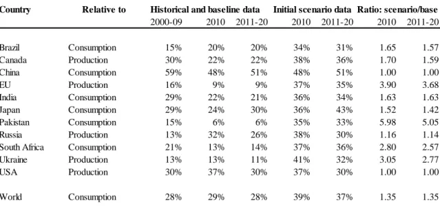
In the AGLINK-COSIMO data, global stocks at the end of marketing year 2010 were 29% of global use, and this ratio is not projected to rise over the ten year Outlook period (Table 1). Among the countries targeted in this experiment, only China and the United States surpass the 36% minimum wheat stocks imposed at the start of the projection period. Stocks are assumed to be higher in other countries, although such changes are not entirely consistent with historic stock ratios. The alternative lower threshold of 20% is more in line with historical patterns for some countries, although clearly too low for others.

Table 1. Experiment stock ratios with 36% minimum

Source: Historical and baseline data of OECD-FAO (2011), and other columns are calculated here as described in the text.

Another technical point is that the model is recalibrated to these higher initial stocks. To ensure comparable starting points with the stochastic baseline projection of world wheat prices, the proposed analysis assumes that higher stocks are on hand initially and that they are the target level chosen or demanded (as compared to the observed lower level). Although a technical issue, the assumption about where to put the demand curve relative to the imposed higher initial stock level can have important implications once the

model simulations commence.13 One alternative approach would be not to recalibrate the

model to the assumed stock levels. In that case, there would be no additional demand for

13. _{The stocks on hand at the start of the first year of a projection are always exogenous, typically}

equal to the observed data. In this case, beginning stocks of the first year are set higher in order to raise the stocks-to-use ratio to the minimum level, if observed stocks fall short of this minimum. For each year of the projection period simulations, stocks are endogenous; they are just started at a higher initial level. Once the model is simulated for the projection period, the stock level in the output data will always be on the recalibrated stock demand curve that is consistent with the higher level of stock demand assumed in this scenario.

Country Relative to 2000-09 2010 2011-20 2010 2011-20 2010 2011-20 Brazil Consumption 15% 20% 20% 34% 31% 1.65 1.57 Canada Production 30% 22% 22% 38% 36% 1.70 1.59 China Consumption 59% 48% 51% 48% 51% 1.00 1.00 EU Production 16% 9% 9% 37% 35% 3.90 3.68 India Consumption 29% 22% 21% 36% 34% 1.63 1.63 Japan Consumption 29% 24% 30% 36% 43% 1.52 1.42 Pakistan Consumption 15% 6% 6% 35% 33% 5.98 5.05 Russia Production 13% 32% 26% 38% 30% 1.16 1.14

South Africa Consumption 21% 13% 14% 37% 36% 2.80 2.57

Ukraine Production 13% 13% 11% 41% 32% 3.05 2.77

USA Production 30% 37% 30% 37% 30% 1.00 1.00

World Consumption 28% 29% 28% 39% 37% 1.35 1.35

(18)

stocks at any given price, just more stocks happen to be on hand at the start of the projection period. These stocks would be sold off quickly, driving price down temporarily, until markets would return to the stochastic baseline combinations of prices and stock levels. If constructed in this way, results would show what happens if additional wheat quantities appear on world markets, but it would not estimate the impacts of a willingness to hold stocks at levels consistent with historical averages. Another approach to this scenario would be to increase stock demand, but not initial stocks. In that case, the assumed willingness to hold more stocks at any given price would lead to greater global demand as stocks are built. The world wheat price would rise temporarily in this case. This initial impact could obscure the impacts on volatility, so the results over a ten-year period might not focus clearly enough on the impact of current low stocks. Moreover, unless stock rules are delineated, and costs tracked, the outcome would not be a good guide for market observers who question the role of public policy to support buffer stocks. However, these practical considerations of a more complex system of public stockholding policy are considered in the next scenario.

A hypothetical international buffer stock scheme

In this scenario, a stylised buffer stock agreement is assumed to exist between a subset of wheat exporters and importers to hold and release stocks in an attempt to condition the market price in a coordinated way in order to avoid large world wheat price

swings.14

A critical issue with buffer stock schemes are the market intervention or price rules governing stock building and sales and whether they evolve with the size and condition of

the market. In this stylised experiment, the buffer stock rules are set ex post, in a sense.

After looking at the stochastic baseline simulation, we set a price band that is approximately centred on the average stochastic baseline price, and that has sufficient width that stock sales and purchases effectively target the extreme cases. Recognising the sensitivity of results to the rules chosen, an alternative case is explored with a different price band. In both cases, this hypothetical band is chosen to represent an international agreement without considering the exact mechanisms of coordination, side-stepping practical questions addressed by other OECD research (Gilbert, 2011). The notion of socially optimal stocks is not explored.

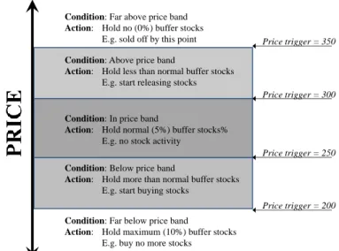
The rules are characterised by four key parameters relating to the price and two relating to stock levels. Consider what happens in one year if the price in the previous year was in the range deemed acceptable with normal buffer stocks on hand (Figure 4). First, if the price rises above USD 300 per tonne, buffer stocks begin to be released. Second, by the time the price rises to USD 350 per tonne, then all buffer stocks will have been released in the effort to mitigate the price surge. Third, if the price declines, then a price of USD 250 requires purchases or acquisition of stocks to help raise prices above this lower trigger level. Fourth, at USD 200, the buffer stocks hit their maximum allowed limit and further purchases or stock acquisition is stopped. This raises the question of quantity parameters, of which there are two. One determines the maximum allowed buffer stocks, 10% of use (including trade) ratio, to be acquired and held. The second

14

It should be noted that this is a very stylised and perfectly designed buffer stock scheme in which the price band is chosen to fit the stochastic price outcomes and in which all participants play exactly according to the rules, something that has not always occurred in the history of ICAs. Furthermore the noted limitations of using annual data may also be more important in this kind of experiment where periodic price surges/falls occur within particular years.

(19)

relates to the quantity of normal buffer stocks, 5% of use, to be held if price is within the band.

Figure 4. Buffer stock scheme rules about price band and stock levels assuming normal buffer stocks are on hand initially

The participating countries in this buffer stockholding scheme are assumed to be Argentina, Australia, Canada, Egypt, the European Union, Indonesia, Japan, Korea,

Malaysia, Mexico, Pakistan, Russia, Ukraine and the United States.15 A key assumption

about the stylised wheat stockholding scheme is that countries buy or release buffer stocks in their domestic markets; based on the application of the wheat stock acquisition rule and the world wheat price, these countries buy or release stocks on their internal markets. By locating the stocks in specific countries – an advantage of a large model such as the one used here – the wheat buffer stocks scheme scenario has a dose of reality that may not be true for analyses that treat buffer stocks as though they are bought and sold in world markets, perhaps implying some multinational stock-holding entity or that stocks are held at ports ready for export or import. In the present treatment, the countries in the hypothetical scheme own the stocks, and the stocks acquisition and release affect their domestic markets first. Intervention in local markets will affect world markets to the extent that traders are able to take advantage of any arbitrage opportunities. In some instances, their ability is curtailed by policies, such as tariff-rate quotas, so impacts in domestic markets in these cases may become pronounced before affecting trade, and world markets. Another fundamental point is that a stockholding scheme might be cast as a global enterprise tied to world market prices, as in the hypothetical scenario explored here, or as a more limited stock policy that offsets specific events that disrupt food consumption in a particular location or region.

15. _{The list of participating countries is not identical to the previous list for the higher stock}

scenarios. The choice is motivated in part for technical reasons, namely the fact that introducing new buffer stocks does not depend on existing stock demand equations, and should not affect results substantially.

Condition: Above price band

Action: Hold less than normal buffer stocks E.g. start releasing stocks Condition: Far above price band Action: Hold no (0%) buffer stocks

E.g. sold off by this point

Condition: In price band

Action: Hold normal (5%) buffer stocks% E.g. no stock activity

Condition: Below price band

Action: Hold more than normal buffer stocks E.g. start buying stocks

Condition: Far below price band

Action: Hold maximum (10%) buffer stocks E.g. buy no more stocks

Price trigger = 250 Price trigger = 350

Price trigger = 200 Price trigger = 300

(20)

Box 2. Summarising stochastic simulation output

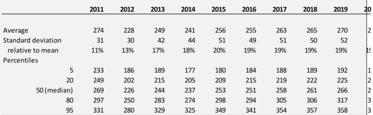
Stochastic simulations of AGLINK-COSIMO generate hundreds of values for prices and quantities, with each solution representing a ten-year outlook projection contingent on a particular set of exogenous shocks. Summary statistics represent the results of these simulations. For example, the baseline data for the world wheat price are summarised using a few key statistics (Table 2.1). The average value of all the hundreds of wheat price observations in marketing year 2020/21 is USD 272 per tonne. The standard deviation of these results, a measure of how widely distributed they are, is 51, which equals 19% of the average value. The percentiles are another way to look at the dispersion, but also to understand better the extreme values. (Ranking all the 2020 wheat prices, the value that is 5% from the bottom is USD 196 per tonne and USD 364 is 5% from the top. The mid-point or median value is USD 268 per tonne.)

Comparing the average and the median and looking at the percentile data suggest an asymmetric distribution. The median is a bit lower than the mean, so there are more values below the average but the high values are further from the mean. Comparing the 5th and 95th percentiles with the median, the 95th percentile value in 2020 is farther from the median than the 5th percentile value. Thus, it appears that the values at the extreme upper end of the range tend to stand out.

Table 2.1. Baseline world wheat price, USD per tonne.

Source: Summary statistics of model simulation output.

The OECD (2010) used a measure of year-over-year price changes to estimate price volatility:

.

The median value of this calculation is used here to compare the results among these scenarios in terms of the impacts on year-over-year changes in the world wheat price at the end of the projection period. The stochastic baseline value is 9.4%.

These measures of volatility allow the reader to assess the distribution of simulated wheat prices using the mean, the standard deviation, the percentiles, and the year-over-year variation. Each measure has its uses. For example, the standard deviation is a better measure of dispersion overall, but the percentiles help to compare the effects of a scenario at the price extremes as well as at and near the median. To facilitate communication, this selection of volatility measures will be used to characterise the results of each scenario.

A technical point is that there is no displacement of private stocks by the buffer stock scheme. In reality, the presence of a buffer stock scheme that is intended to limit price movements will decrease the incentive for private agents who might otherwise try to build stocks when prices are low in order to have commodities available to sell when prices rise. Although wheat stocks, apart from the new buffer stocks do respond to price signals in these simulations, there is no fundamental change imposed that could reflect

2011 2012 2013 2014 2015 2016 2017 2018 2019 2020 Average 274 228 249 241 256 255 263 265 270 272 Standard deviation 31 30 42 44 51 49 51 50 52 51 relative to mean 11% 13% 17% 18% 20% 19% 19% 19% 19% 19% Percentiles 5 233 186 189 177 180 184 188 189 192 196 20 249 202 215 205 209 215 219 222 225 228 50 (median) 269 226 244 237 253 251 258 261 266 268 80 297 250 283 274 298 294 305 306 317 310 95 331 280 329 325 349 341 354 357 358 364

(21)

how they respond to the reduced profitability of storing wheat. Stocks continue to be held, usually based on current price relative to an expectation of future price that is based on a moving average of recent prices. To the extent that private agents reduce their stocks, this response will offset some of the new buffer stocks, reducing their effectiveness without decreasing the costs to taxpayers.

3. Market sensitivity as developing country demand becomes less elastic

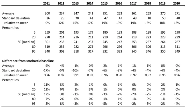
This scenario addresses the question of how sustained high income growth in the BRIC countries that reduces responsiveness of demand to price changes (but not overall consumption levels) affects world commodity market volatility, measured with annual prices, over the projection period. The results of the stochastic experiments suggest that the effects are modest over the ten-year projection period. The BRIC scenario results in somewhat greater volatility in year-over-year price changes, at 10.2%, relative to the stochastic baseline value, 9.4%, taking the median value in marketing year 2020 (Box 2). The changes in world wheat price average, standard deviation, and percentile values are all quite small, but move in the same direction (Table 2). The small effect on average prices reflect the design of the scenario, in that the original price level is largely maintained in order to focus on the implications of changing demand elasticities on price variation, so the responsiveness of demand changes but there are no shifts in food or feed demands for wheat.

Table 2. BRIC scenario world wheat price, USD per tonne

Source: Summary statistics of model simulation output.

There are at least two important reasons for the small scale of the impact of BRIC income growth on world wheat market sensitivity. One is that the time frame is short for the process. The exact link between average per capita income and sensitivity of demand is not known, but the estimates used here are based on a gradual process. A key underlying assumption is that this is a smooth process. However, it may be that there are

2011 2012 2013 2014 2015 2016 2017 2018 2019 2020 Average 274 228 249 241 256 255 263 265 270 272 Standard deviation 31 30 42 44 51 49 51 50 52 51 relative to mean 11% 13% 17% 18% 20% 19% 19% 19% 19% 19% Percentiles 5 233 186 189 177 180 184 188 189 192 196 20 249 202 215 205 208 215 219 222 225 227 50 (median) 269 226 244 237 253 251 258 261 266 268 80 297 250 283 274 298 294 305 306 316 310 95 331 280 329 326 349 341 354 357 358 366

Difference from stochastic baseline

Average 0.00% 0.00% 0.00% -0.01% -0.01% -0.02% -0.03% -0.03% -0.01% -0.03% Standard deviation 0.00% 0.02% 0.06% 0.08% 0.09% 0.12% 0.16% 0.18% 0.29% 0.27% relative to mean 1.000 1.000 1.001 1.001 1.001 1.001 1.002 1.002 1.003 1.003 Percentiles 5 0.00% -0.01% -0.02% -0.05% -0.06% -0.08% -0.15% -0.14% -0.05% -0.17% 20 0.00% -0.01% 0.00% -0.03% -0.04% 0.03% -0.07% -0.04% -0.09% -0.09% 50 (median) 0.00% 0.00% -0.01% 0.00% -0.03% -0.03% -0.03% -0.03% -0.02% -0.06% 80 0.00% 0.00% 0.00% 0.03% -0.04% -0.05% -0.01% 0.09% -0.04% 0.01% 95 0.00% 0.01% 0.00% 0.01% 0.05% 0.06% -0.02% 0.04% 0.00% 0.39%

(22)

sharper distinctions in demand response at different stages of development, and if so then passing a break point might cause a larger change in overall market response.

The other reason is that the test focuses on four specific countries, not all developing countries, and the domestic markets of these countries are not well integrated with world markets in every case. China and India have traditionally held self-sufficiency and domestic price management as focal points of their staple grain policies, with less regard to the potential to achieve some goals more efficiently by allowing increased trade. In view of their large populations and policies that hinder trade, the effects of changes in demand in these countries may be more pronounced in domestic markets, rather than on world markets to which they turn periodically to dispose of surpluses or supplement supplies. The Russian Federation’s ambivalence about trade and its reputation as a reliable supplier is demonstrated by its market interventions – wheat export bans – when prices spiked in 2007-08 and again in 2010. While Brazil maintains a less interventionist stance, the number of consumers is much smaller than the population of China or India.

All food demand elasticities in these countries are changed in this scenario, not just wheat food demand elasticities. The wheat price and quantity changes represented here also include the indirect impacts caused by changes in the prices of other agricultural commodities on wheat markets. The impacts on the world prices of rice and coarse grains are of a similar order of magnitude as the wheat price changes. The distributions of world rice and coarse grain prices also broaden.

The small effects on world prices should not be interpreted to mean no important effects at all. Looking in more detail at the case of India's food use of wheat, for example, shows that there are important changes (Table 3). The consequence of less responsive demand in India is exactly that: changes in market prices cause smaller changes in consumption. The range of variation in India’s wheat food use narrows more and more as demand becomes less elastic. Looking at the standard deviation, it is 1% lower than the stochastic baseline value in 2012 marketing year, and 7% lower in 2020. The percentile

data show the same pattern. The 5th percentile is higher by 0.02% in the 2012 marketing

year and 0.27% higher in 2020; and the 95th percentile is 0.04% lower in 2012 and 0.49%

lower in 2020. A high price has less power to push down food use in India as income rises, and a low price gives a smaller incentive for more consumption as consumers become less poor or more affluent over time.

The effects are small over the ten year period, but assumed income growth over time causes world commodity markets to become less and less responsive to prices. The changes in price ranges would presumably be greater if the analysis were extended farther into the future. The changes in elasticities over this period are between fifth and one-third of the estimated changes in elasticities if BRIC per capita GDP were USD 35,000, a level that would put these four countries firmly within the GDP range of OECD members. Changes in price levels would probably be apparent if the initial food use volumes were allowed to change rather than imposing the same baseline starting values to focus on volatility. Large changes could lead to other questions. For example, if the range of price variation increases dramatically, then will more private stocks be held to take advantage of the greater opportunities for arbitrage? If price levels rise substantially, then how will input suppliers respond over a long-run horizon in terms of developing new management techniques, seed varieties and other productivity enhancements? At what point would changing circumstances lead to changes in policy mechanisms, or even more fundamental restructuring of policy? Thus, while results here support the view that income grown in developing countries seems likely to have limited impact on market volatility in the