DOI 10.1007/s10827-007-0034-x
The neuronal dynamics underlying cognitive
flexibility in set shifting tasks
Anja Stemme·Gustavo Deco·Astrid Busch
Received: 5 August 2006 / Revised: 13 March 2007 / Accepted: 19 March 2007 / Published online: 18 May 2007 © Springer Science + Business Media, LLC 2007
Abstract The ability to switch attention from one
as-pect of an object to another or in other words to switch the “attentional set” as investigated in tasks like the “Wisconsin Card Sorting Test” is commonly referred to as cognitive flexibility. In this work we present a biophysically detailed neurodynamical model which illustrates the neuronal base of the processes related to this cognitive flexibility. For this purpose we conducted behavioral experiments which allow the combined evaluation of different aspects of set shift-ing tasks: uninstructed set shifts as investigated in Wisconsin-like tasks, effects of stimulus congruency as investigated in Stroop-like tasks and the contribution of working memory as investigated in “Delayed-Match-to-Sample” tasks. The work describes how general experimental findings are usable to design the archi-tecture of a biophysical detailed though minimalistic model with a high orientation on neurobiological find-ings and how, in turn, the simulations support
exper-Electronic supplementary material The online version of this article (doi:10.1007/s10827-007-0034-x) contains
supplementary material, which is available to authorized users.
Action Editor: Peter Dayan A. Stemme (
B
)·A. BuschDepartment Psychologie, LMU Munich, Leopoldstr. 13, D-80802 Munich, Germany e-mail: [email protected], [email protected]
G. Deco
ICREA Research Professor, Computational Neuroscience, Universitat Pompeu Fabra, Passeig de Circumvallació 8, 08003 Barcelona, Spain
e-mail: [email protected]
imental investigations. The resulting model is able to account for experimental and individual response times and error rates and enables the switch of attention as a system inherent model feature: The switching process suggested by the model is based on the memorization of the visual stimuli and does not require any synaptic learning. The operation of the model thus demonstrates with at least a high probability the neuronal dynam-ics underlying a key component of human behavior: the ability to adapt behavior according to context requirements—cognitive flexibility.
Keywords Cognitive flexibility·
Wisconsin Card Sorting Test·Set shifting task· Working memory·Visual attention·PFC· Neurodynamical model
1 Introduction
A range of neuronal models have been developed for set shifting tasks comparable to the “Wisconsin Card Sorting Test” (WCST, Dehaene and Changeux
1991; Berdia and Metz1998; Amos2000; Rougier and O’Reilly 2002; Rougier et al. 2005) in order to gain an understanding of the neurodynamics underlying the (uninstructed) shift of attention. The WCST (see e.g. Milner1963) requires subjects to sort cards containing colored shapes according to one of three possible rules (usually color, shape, number). If the chosen sorting criteria was correct participants received the feedback “correct” for a placed card. After a certain number of correct trials the valid sorting rule changes without ex-plicit notice. Thus, subjects are provided with the feed-back information “wrong” and are required to adapt
their response behavior for the next trial by choosing a different sorting criteria or new relevant rule, re-spectively. Of central interest within this experimen-tal design are so-called “perseverative” errors which means that subjects do not switch to a new relevant rule following the feedback “wrong” but continue to give their answers according to the previously correct rule. Thus, perseverative errors obviously seem to indicate a kind of missing “cognitive flexibility.”
The WCST is well known to be sensitive for various kinds of patients’ disorders and especially dysfunctions of the prefrontal cortex (PFC) seem to be reflected in corresponding experimental results i.e. a compara-tively high amount of perseverative errors (e.g. Miller and Cohen 2001). These findings appear to apply for patients with frontal lobe damages (first examined by Milner 1963) as well as for patients suffering from Schizophrenia or Parkinson’s disease (see for example Everett et al. 2001; Owen et al. 1993). Accordingly, neuronal modeling work focussed on the investigation of perseverative errors and their relationship to PFC dysfunction. However, this focus bears some problem-atic aspects:
– First of all, errors are committed as well by healthy subjects. These errors might be perseverative but as well “non-perseverative” and hence more related to the degree of participants’ attention. To ensure plausibility it is desirable that neuronal models ac-count for these different types of errors which are committed (as well) by healthy subjects i.e. by an unlesioned or unimpaired model.
– Further more, recent research revealed that errors more related to attentional questions might to a significant part be responsible for the impaired per-formance of patients with frontal lobe damages (e.g. Barceló and Knight2002). Moreover, experimental results especially for schizophrenic patients are not unique; hence schizophrenics might show persever-ative behavior (e.g. Kolb and Wishaw1983; Everett et al.2001) or not (e.g. Goldstein et al.1996; Landro et al.2001). This divergence stresses the importance to examine experimental results in detail and to consider the specific error context in order to design appropriate models.
The neuronal model for the WCST presented by Dehaene and Changeux (1991) considered persever-ative and what they called “random” errors only for lesioned models. Thus the unimpaired model did not produce any errors at all. However, the authors were one of the first to suggest a neuronal model for the WCST and delivered valuable hints to understand the neuronal operations underlying this test. As such, they
successfully predicted the existence of neuronal rule coding clusters kind of which were later detected by White and Wise (1999). These “rule” neurons are responsible for the abstract properties of the visual objects and form an essential part of every model suggested for set shifting tasks including the model presented in this work.
Berdia and Metz (1998) and Amos (2000) simu-lated different error types by modifications of explicit gain and noise parameters. However, such an approach somehow hides the subject of interest: How are these parameters to be translated into neuronal operations?
The models presented by Rougier and O’Reilly (2002) and Rougier et al. (2005) produced as well sys-tem inherent attentional errors referred to as “back-ground” or “occasional” errors. These system inherent attentional errors were considered as a desired model feature but the authors immediately faced the next difficulties which were related to the handling of the occasional errors. The reason is hidden in the imple-mentation of the switching process. For this process all models, named so far, rely on the mechanism of “direct rule inhibition” partly combined with an addi-tional “gating mechanism” (Rougier and O’Reilly2002; Rougier et al.2005). This means that following a nega-tive feedback (representing the feedback information “wrong”) the active model rule is directly inhibited (and in case the gating mechanism activated) which enables the activation of a different rule for the sulation of the next trial. The consequence of this im-plementation is that following every single (attentional) error the model enters into the process of activating a different rule for the next trial. This handling seems to be inappropriate for attentional errors and leads to subsequent errors in the following trials. Thus, the simulation results do not show single attentional errors but only error sequences of at least two errors. This circumstance might even lead to an overall inadequate amount of attentional errors (Rougier and O’Reilly
2002; Rougier et al. 2005, page 507 and supplemental material). To solve this problem the authors chose to delay the feedback information. Hence, the feedback message “wrong” following an incorrect model answer was delivered to the model only after two errors in a row otherwise the feedback information “correct” was provided. Thus, these models do not enter into the process of rule switching following single attentional errors. As a necessary consequence the amount of per-severative errors increased: Now at least two errors in a row are necessary for every switch of the valid rule.
The key questions behind these considerations turn out to be: Do subjects commit single attentional errors and are subjects able to switch the sorting criteria,
i.e. the relevant rule, after a single feedback message “wrong?” It seems unlikely to assume that single atten-tional errors are impossible or that the attenatten-tional set is switched only after two errors in a row. Hence, these simple error context considerations represent a hint that neuronal models presented so far for set shifting tasks face some important limitations with respect to their ability to simulate human behavior. Moreover, the considerations indicate that the chosen neuronal concepts thought to explain the shifting process might be inappropriate.
To examine these questions experimentally and de-velop an according neuronal model we designed a new type of experiment which combines different as-pects of set shifting tasks though using a rather simple setup to enable realistic neurodynamical simulations. The experimental setup combines a visual “Delayed-Match-to-Sample” task with a Wisconsin-like paradigm (WDMS task): Two visual stimuli, consisting of simple colored shapes, are presented to the subjects, separated by a delay. Following the presentation of the second stimulus the participants are required to state whether the stimuli matched with respect to a given criteria or did not match. We chose two different possible matching criteria and changed the relevant one at ar-bitrary intervals without explicit notice (uninstructed Wisconsin-like set shift). This setup allows to inves-tigate effects of stimulus congruency (comparable to Stroop tasks) as well as the working memory contribu-tion (DMS task) with respect to the shift of attencontribu-tion. Hence, the key performance measures were chosen to be subject response times in dependence of stimulus congruency and relative to the set shift. Further more different error types were classified and analyzed. In considering not only experimental average results but as well individual variations we obtain a rather detailed description of human behavior compared to previous studies. The rather simple task design has, more over, the advantage that the neuronal dynamics are explore-able by a comparatively simple model design. Further-more, the WDMS comprises all elements present in set shifting tasks (attend to a selected feature of a multi-featured stimulus and change this attention on an im-plicit request) and might therefore even be suitable to clarify diverging WCST results by providing the possi-bility to differentiate in a greater detail between perfor-mance components more related to working memory or attention, for example, especially in conjunction with according neurodynamical simulations.
Against the background of the described problems existing set shifting models face we decided to start the modeling approach rather from the scratch. Therefore we used a biophysical detailed neurodynamical model
for the task simulation. Although this model, based on “Integrate-and-Fire” neurons, uses as well several simplifications the biophysical description of neuronal activity approximates natural neuronal activity compar-atively accurate (see e.g. Tuckwell 1988; Brunel and Wang 2001). We thus aim to investigate how
neu-rons might cooperate to form cognitive flexibility given
the rather detailed description of challenging neuronal properties.
While using a rather detailed and complex descrip-tion of neuronal behavior we looked at the same time for a rather simple neuronal organization leaned on neurophysiological findings. Thus the model comprises a minimal number of neuronal pools responsible for rule specific activity (as detected for example by White and Wise1999) and object specific activity (e.g. Rainer and Miller2002). The neurons are coupled with differ-ent connection strengths via the three most common cortical connection types found so far. The connection strengths are supposed to remain fixed during the simu-lation as there is no evidence that every rule switch has to be learned again and again in a single experiment. Without any further algorithmic additions the model itself, the neuronal organization of rule and stimulus specific neurons, is responsible for the completion of set shifts and hence an adequate set of weights has to be chosen.
Here, an asymmetric set of weights is suggested to account for a memory based switching process where stronger feedforward connections between rule and stimulus specific neurons are responsible for the main-tenance of a rule and stronger feedback connections are responsible for the selection of an alternate rule and thus for the shift of attention. Opposed to previous models, the focus of the switching procedure thereby moved from the rule neurons to the stimulus neurons. This is a rather important aspect: The center of the switching procedures is build by the stimulus neurons which obsoletes the usage of a “direct rule inhibition” algorithm and thus avoids above described problems.
An important model feature is represented by the consideration of external input from other cortical ar-eas to the model neurons. This input is important for the operation of the model and accounts as well for the observed high degree of cortical connectivity. The input varies randomly within a certain range and may thought to reflect a kind of attention payed to the actual task. Fluctuations in this external input are shown to be responsible for different types of errors. These errors thus represent a system inherent model feature and are comparable to those errors committed by healthy subjects during the experiments. The response times generated by the model are dependent on stimulus
congruency comparable to the effects observed in Stroop-like tasks (see e.g. Monsell 2003; Egner and Hirsch 2005) and to the response times generated by the subjects in the investigated WDMS task. The en-tire model represents an extension of the framework presented by Brunel and Wang (2001) which has been applied successfully as well to the description of selec-tive working memory and attention (Corchs and Deco
2002; Deco and Rolls2003; Deco et al.2004; Almeida et al.2004; Deco and Rolls2005). The high degree of detail used by biophysical models enables as well the calculation of fMRI signals, for example, as already demonstrated for set shifting tasks in Stemme et al. (2005).
With respect to the establishment of the neuronal connections within the model we left aside the ques-tion how these connecques-tions might be learned (analyzed for example by Rougier and O’Reilly 2002; Rougier et al.2005). Rather we focussed on the development of a neuronal model capable to explain the set shifting process and its relations to attention and working mem-ory with a high degree of neurobiological orientation. The entire complex of set shifting tasks and biophysical models is discussed in detail as well in Stemme (2007).
2 Materials and methods
2.1 Wisconsin-DMS experiments
2.1.1 General setup
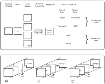
In Fig.1the experimental setup is depicted. We used a “Delayed-Matching-to-Sample (DMS)” design in com-bination with a set-shifting task: A sample display was shown for 500 ms, followed by a fixation delay of 1000 ms, followed by a test display which was presented until the subjects responded by key press (“y”–yes or “n”– no; yes–sample and test display matched with respect to the valid rule, no–sample and test display did not match according to the currently valid rule). Afterwards a feedback message informed the subjects whether their response was “correct” or “wrong.” The feedback mes-sage was presented for 1,500, 1,000 or 500 ms (WDMS I, II, III). The stimuli in the sample and test display con-sisted of colored, oriented rectangles of different sizes which were presented at one of 64 different locations on the screen. Only one of the rectangles was presented in sample and test display at a time. The subjects had to discriminate between two different possible rules: Same position on the screen (called further on “space rule”) or same object presented in sample and test display (with respect to all feature dimensions; called
Fig. 1 Setup of the “Wisconsin Delayed-Matching-to-Sample” experiments (top) and example trial sequence (bottom). The trial sequence shows a rule change in the second trial; the object rule was valid in the first trial. Starting with the second trial the new valid rule is the space rule
“object rule” in the reminder of the document). After an arbitrary number of correct trials (3, 5, 7, 9 or 11 not necessarily consecutive correct trials) the valid rule was changed without notice (Wisconsin-like paradigm). In this case the subjects received the feedback message “wrong” although they responded correctly according to the valid rule in the previous trial (see Fig. 1, bot-tom). The stimulus material (colored, oriented rectan-gles of various sizes) was chosen in order to prevent verbalizations of the subjects to a great extend. The rule was changed at arbitrary intervals to prevent subjects from counting and estimating the rule switch trial. Fur-ther on we refer to the trials between two rule changes as “maintenance phase.” I.e. after subjects successfully acquired a new rule their major task is to maintain this rule until the next requirement for a set shift occurs which was indicated by the feedback “wrong.”
2.1.2 Stimulus congruency
An important point for the analyzation of response times is the stimulus congruency and hence the discrim-ination of the possible match conditions of the stimuli presented in the sample and test display:
both: The stimulus presented in the sample display and the one presented in the test display are identical with respect to both rules.
match: The stimulus presented in the sample display matches the test display stimulus only with respect to the currently valid rule (i.e. the irrelevant stimu-lus dimension does not match).
nonmatch: The stimulus presented in the sample dis-play does not match the test disdis-play stimulus with respect to the currently valid rule (i.e. the irrelevant stimulus dimension matches).
none: The stimulus presented in the sample display and the one presented in the test display are different with respect to both dimensions.
Trials with “both” and “none” conditions are also re-ferred to as trials with congruent stimulus conditions (short “congruent trials”) whereas trials with “match” and “nonmatch” conditions are summarized as trials with incongruent stimulus conditions (short “incongru-ent trials”). This differ“incongru-entiation is very similar to the stimulus differentiation tested in Stroop-like tasks (see e.g. Monsell2003) though the present design provides us with further differentiation possibilities (two differ-ent congrudiffer-ent conditions and two differdiffer-ent incongrudiffer-ent conditions) whereas Stroop tasks only permit the com-parison of “both” conditions with “match” conditions however with a stronger interference of the possible rules. However, with the current form of the WDMS task we do not consider effects with respect to the “overtraining” of one stimulus dimension against the other as in the original Stroop task (Stroop 1935). Rather both relevant stimulus dimensions proved to be of equal non-interfering complexity comparable to the sorting criteria in the original WCST.
2.1.3 Error types
For the analysis of error rates the following error types were differentiated:
Rule acquisition errors (AQ): These are the first errors of an experiment or a trial block within an experi-ment where subjects try to find out the first valid rule.
Rule change errors (RCE): These are necessary errors subjects make (in the rule change trial) when the valid rule is changed without notice (see Fig. 1, bottom, trial 2).
Errors in the context of a rule change(RCF): These are errors occurring after the valid rule was changed and before the new valid rule is considered to be definitely established by the subjects. The establish-ment of a new rule is assumed to have happened after three consecutive correct answers1 (start of
“maintenance phase”). RCFs2might be considered as well as “perseverative errors.”
1Similar to Konishi et al. (1999) and Nakahara et al. (2002) who
considered a new rule to be established after three correct trials.
2RCF = Rule Change Follow up.
Unmotivated errors (UE): These are errors made after a new rule is considered to be established. We consider these errors to be related to the attention of the participants and call them “unmotivated” because the exact reason for these errors is so far unclear. As outlined above they are called also “random” “occasional” or “non-perseverative” errors in the literature.
Errors in the context of an unmotivated error (UEF): These are errors following an unmotivated error. Similar to RCFs, errors were considered as UEFs before the subject again responded correctly in
three consecutive trials after an UE.
UEs and UEFs were distinguished to examine the context of a single unmotivated error. We hypothesized that the reason for an unmotivated error might well be a spontaneous rule change of the subject. Thus we considered again three consecutive correct trials to be necessary for the correct rule to reestablish after an unmotivated error occurred. RCEs do not represent errors in its original sense. Thus they were excluded from the analysis.
2.1.4 Experimental time course
For every experiment the participants had to complete ten experimental blocks. After every block participants had the possibility to pause for a self-determined period of time. One single block required to complete nine rule changes leading to a total number of about 850 trials per participant per experiment. In 75% of the trials incongruent stimulus conditions were used.
2.1.5 Participants
Forty healthy subjects participated in three variants of the experiment with feedback times of 1,500, 1,000 and 500 ms (WDMS I–13 participants , WDMS II–14 partic-ipants, WDMS III–13 participants) without additional inter trial time. Thus after completion of the feedback time the next trial started immediately.
2.2 The neurodynamical model
2.2.1 A biophysically detailed approach
The neurodynamical model used for the simulations (described as well in Stemme et al. 2005; Stemme
2007) is based on the framework first introduced by Brunel and Wang (2001). The model represents a selected cortical area and consists of two differ-ent types of neurons, 80% excitatory pyramidal cells
and 20% inhibitory interneurons, consistent with neu-rophysiological findings (Abeles 1991). The neurons are grouped into two appropriate types of pools: ex-citatory and inhibitory pools. Each neuron is mod-elled as an “Integrate-and-Fire” neuron taking into account three different synaptic connection types: two excitatory—AMPA and NMDA connections—and one inhibitory—GABA. The three different synaptic con-nection types are represented and computed using equivalent electrical circuits, consisting basically of a resistance parallel to a conductance with type specific parameter values for conductivity and resistance.
Every neuron receives a certain background input from neurons outside the network modelled. The cere-bral cortex is highly connected and thus the simulation of a “closed” cortical area would be unrealistic. For the approximation of the background input, it is taken into account that neurons always show a certain level of activity, i.e. a spiking rate of approximately 3 Hz for pyramidal cells and 9 Hz for interneurons, which is called the “spontaneous rate,” (see e.g. Wilson et al.
1994). Accordingly, the external background input is modeled as an AMPA-mediated Poisson train of spikes arriving from Next=800neurons with a rate of 3 Hz. Thus, the total background noise each modeled neuron receives comes out toνext=800∗3 Hz=2.4kHz.
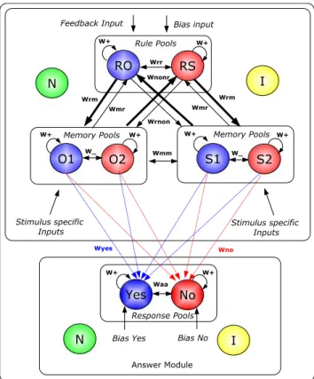
The overall model (see Fig.2) is divided into two, loosely coupled modules each of which has its own non-selective (Fig.2, N) and inhibitory (Fig. 2, I) pool of neurons:
– A main module, covering rule and memory pools which is responsible for the maintenance of the active rule and the memorization of the presented stimuli during the task and
– an answer module, responsible for the explicit initi-ation of the model answer.
The major focus of this work is constituted by the main module which covers 1600 excitatory neurons (NE) and 400 inhibitory neurons (NI) whereas the answer module consists of 800 excitatory and 200 inhibitory neurons. Each pool selective for a specific function within a module consists of 100 excitatory neurons for the main module and 50 neurons for the answer module. The remaining excitatory neurons of a module are organized into the pool of non-selective neurons (not all neurons within a given cortical area respond to a specific task, see e.g White and Wise1999). This pool also introduces some noise and supports the generation of the almost Poisson-like firing patterns of the neurons in the simulation which is a property of many neurons observed in the cortex (Brunel and Wang 2001). The
Fig. 2 The neurodynamical model for the simulations consisting of a main module (2,000 neurons) and an answer module (1,000 neurons). I = Pool of inhibitory neurons. N = pool of non-selective neurons. RO = neuronal pool for the object rule, RS = pool for the space rule. O1/O2 = object pools, representing two different objects; S1/S2 = space pools, representing two different positions on the screen. Each selective pool of the main module comprises 100 neurons. For the answer module the yes/no pools consist of 50 neurons each. All neurons receive an mediated external input of 2.4 kHz. Additional external AMPA-mediated input is provided to the pools in order to simulate the desired task (refer to the text)
inhibitory neurons are grouped to form one inhibitory pool which implements a global competition between all neurons within a module or a given cortical area, respectively, again consistently with experimental find-ings. The network of neurons within a module is fully connected with different connection strengths.
The identification of the various pools within the main module is supported by single cell recordings with behaving monkeys. These recordings showed that single neurons show rule specific (e.g. Wallis et al.
2001; White and Wise 1999) as well as object specific (e.g. Rainer and Miller 2002) activity in a range of behavioural tests. These results led us to the assump-tion that groups of neurons (i.e. the pools) code for specific stimulus features as well as for the more ab-stract rules in the tasks we aim to simulate. Hence, the main module comprises two pools serving as “rule pools,” representing two different, possible active rules
and four stimulus specific pools, representing two times two different stimulus properties: Two different objects (“Object Pools”) which may be presented at two different locations on the screen (“Space Pools”). We also refer to the four stimulus specific pools to-gether as “memory pools” because these pools serve as working memory for the modeled stimulus features. An object at a certain location is presented to the model (e.g. object number one at position number two) by adding an extra Poisson input to the specific pools (ob-ject pool No. 1 and space pool No. 2). For this purpose the external AMPA-mediated input to the neurons within the specific pool is increased to νext+λstimulus. Compared to the background noise,νext=2.4 kHz, the stimulus specific input is rather low:λstimulus=0.15 kHz. The consideration of only two different objects at two different locations enables us already to simulate the principal stimulus sequences as experienced by the human subjects. Contrary to the subjects the neuronal model is not able to cheat or use other cognitive processes besides the ones modeled and thus this re-duction in the number of stimuli does not reduce the simulation capability of the experiment. It is therefore not necessary to consider 64 objects and 64 different locations for the simulations (see as well Stemme2007). To raise and hold competition the rule pools receive continuously a low attentional biasing input, λb ias= 0.07 kHz. One of the rule pools wins the competition and enters into a state of persistant activity with a spik-ing frequency of about 20 to 30 Hz. This active, spikspik-ing rule pool represents the rule “selected” by the model to be currently valid. At the end of a simulated trial
we introduce an unspecific extra external input to the network representing the feedback the model would receive to the previously given answer. The feedback input is provided simultaneously to both of the rule pools, thusνextis increased byλb iasandλf eedb ack. In case of a correct answer we refer to the feedback input as “positive feedback” and “negative feedback” in case of an incorrect answer. However, the feedback input itself is in both cases an external, unspecific AMPA mediated input to both of the rule pools, differing just in the amount of the value. Thereby the positive feedback actually acts as a “strengthener” of a currently active rule pool whereas the higher negative feedback desta-bilizes the rule pools and hence erases any previously persistant activity of any of the two pools.
2.2.2 The rule switching process: memory based set shifting
As depicted in Fig. 2 every rule pool supports “its” memory pools via a comparatively strong weight
wrm>> wrnon (“feedforward” direction). Hence, the object rule pool (RO) provides a higher amount of input to the object memory pools (O1 and O2) than to the space memory pools (S1 and S2). Contrary, in the opposite, “feedback” direction the object memory pools (O1 and O2) provide a higher amount of input to the space rule pool (RS) than to the object rule pool (RO); thuswnonr >> wmr. This asymmetric connection configuration enables the model to switch the rules or shift the set, respectively.
Fig. 3 Illustration of the set shifting process. During the presentation of stimulus 1 (test display) the space rule is active (RS) and the stimulus pools O1 and S1 receive the extra external inputλstimulus. For the delay period the extra input is
removed and the stimulus pool S1 shows delay activity represent-ing the memorization of this stimulus accordrepresent-ing to the valid rule (active pool RS amplifies the activity of pool S1). For the sample display another stimulus is presented to the model represented by an increase in the extra external input to the pools O2 and S1. Following the sample display the negative feedback is provided represented by an increase in the extra external input
to the rule pools (4. picture). During the feedback provision (and as well afterwards) the stimulus pool representing the last relevant stimulus feature (pool S1) keeps its spiking activity. Following the removal of the external feedback input the rule pools return to a spontaneous level of activity where now the input provided by stimulus pool S1 enables the switch of the active rule (5. picture). Due to the connections strengths asymmetry the pool S1 provides an higher amount of input to the object rule pool (RO) than to the space rule pool (RS). Thus we see the object rule pool active (pool RO, 6. picture) for the next trial
The operation of this concept is illustrated in Fig.3: During a trial, the rule pools are constantly active, am-plifying the activity of their according memory pools. Following a model response the stimulus inputs are removed and, depending on the model response, the feedback information provided. After the provision of the negative feedback (for a wrong model answer) the rule pools are destabilized, thus they return to a spon-taneous level of activity. However, the memory pools keep their activity according to the last presented stim-ulus. Due to the continuous supply of the attentional bias (λb ias) the rule pools enter again into a competing stage following the destabilization. In this stage, the previously irrelevant rule pool has an advantage: Be-cause of the connection strength asymmetry this pool receives a higher amount of input from the memory pools compared to the previously relevant rule pool. Thus, the memory pools control the switch to a new valid rule and therefore we call this process a “memory based set shifting process” where the memorization of the last relevant stimulus feature guides the switch to the new relevant rule.
In this approach, the memorization of the abstract rule itself is not responsible for the set shift and hence the focus of the switching concept moved from the rules (as in previous models) to the stimulus features them-selves. Further more, the active spiking rule pool, i.e. the relevant rule, does not inhibit the irrelevant stim-ulus dimension but amplifies the relevant dimension, which represents a suggested mechanism for cognitive control recently supported by neuroimaging studies conducted by Egner and Hirsch (2005). The implemen-tation is consistent as well with the results obtained by Chen et al. (2001) who detected neuronal activity in the prefrontal cortex reflecting irrelevant stimulus dimensions.
2.2.3 Response determination
The model response is linked to the summed spiking rate of all memory pools as all of them are involved in the response generation (relevant and irrelevant mem-ory pools). Figure2(supplemental material) shows an excerpt of the spiking dynamics of the main module pools across several trials and illustrates how the mem-ory pools cooperate to form the model response.
The summed spiking rate, ssr, turns out to be higher for “both” and “match” conditions (“yes”-response necessary) compared to “none” and “nonmatch” cases (require a “no”-response). This circumstance is rea-soned in a kind of spiking rate “constance” across the dimensional memory pools when the same stimulus is presented in sample and test display.
Accordingly, the model response is determinable based on the memory pool activity in the following way:3
– The model response is considered to be “yes” if the ssr crossed a threshold Tyes x number of times: Ryes=ssr>xTyes
– The model response is considered to be “no” if the
ssr stays y number of times below a threshold Tno:
Rno=ssr<y Tno
Further on, an optional minimal spiking rate of the memory pools might be considered in order to generate a neuronal response. This threshold, Tmin, ac-counts especially for the “No”-responses of the model as in this case the spiking rate is required to stay below a certain value. Hence, the threshold Tmin represents the assumption that a certain spiking level might be necessary for the neuronal spiking development to be-come “conscious.” In summary:
Ryes=(ssr>xTyes) (ssr>1Tmin) (1)
Rno=(ssr<y Tno) (ssr>1 Tmin) (2) Response errors committed by the model during the simulations are reasoned in the (system inherent) fluctuations in the external AMPA input (νext). These fluctuations influence the spiking activity of memory and rule pools and thus prevent on the one hand the proper memorization of stimulus features (leading to wrong model responses in the maintenance phase of an active rule4) and prevent on the other hand the
success-ful completion of rule changes (leading to perseverative errors.5 Further more, these fluctuations may lead as
well to arbitrary rule changes during the simulations.6 Thus the model ”generates” attentional errors as well as perseverative errors as a system inherent model feature where none of the error types require an addi-tional handling (as feedback delay, for example) by the model architecture.
2.2.4 Simulation setup
We conducted several simulations comprising 300 trials each. For every simulation we modified the fluctuation
3Please refer to supplemental material for the response pool
configuration.
4An example of the according spiking dynamics is provided in
Fig.3of the supplemental material, trial 98.
5Compare Fig.2(trials 86 and 87) and Fig.3(trial 92),
supple-mental material.
6Spiking dynamics reflecting such arbitrary rule changes are
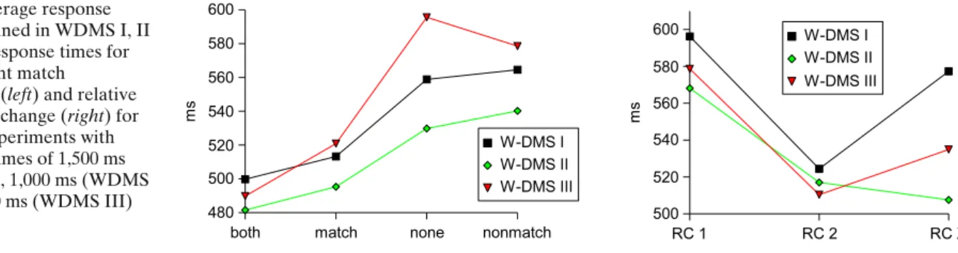
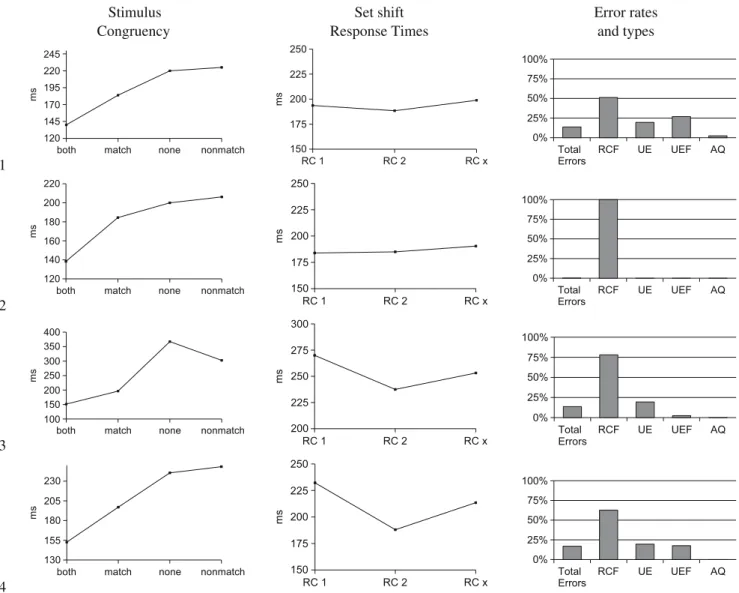
Fig. 4 Average response times obtained in WDMS I, II and III. Response times for the different match conditions (left) and relative to the rule change (right) for WDMS experiments with feedback times of 1,500 ms (WDMS I), 1,000 ms (WDMS II) and 500 ms (WDMS III)
scheme and varied minor model parameters (different possible model options, compare as well supplemen-tal material). The fluctuations in the external AMPA input rely on the performance of a random number generator. Thus, different fluctuation schemes during the simulations are achievable by the usage of different random seeds. Further more, the fluctuations might be kind of “controlled” by a reset of the random generator for every trial within a simulation run. Further infor-mation regarding the concrete model configuration for the simulations is provided as supplemental material (Table4).
3 Results
3.1 Average performance measures
3.1.1 WDMS experiments
Figure 4, left diagram depicts the average mean re-sponse times (RT) for the three experiments7 in dependence of stimulus congruency. For WDMS I, response times for trials with “both”-conditions were significantly lower than response times for trials with “match”-conditions; further on, response times for “both” and “match”-conditions were significantly lower than response times for “nonmatch” conditions but no significant effect arose for the relationship between the response times for “nonmatch” compared to “none” cases. In summary:
– “Yes” responses were faster than “no” responses (mean difference 60 ms, p=0.0008).
– Responses for “both” trials were faster than for “match” trials (mean difference 41 ms, p=0.0008). – For the relationship of “none” to “nonmatch” trials
no significant effect arose.
7All experimental results were determined based on the raw
experimental data (unless otherwise noted) with outlier values (more than±2.5 standard deviation per subject) removed for the determination of response times.
The results for WDMS II and III showed the same pattern of relative response times although the “non-match” response time turned out to be numerically lower than the “none” RT for WDMS III opposed to the other experiments.
Figure 4, right diagram shows the response times relative to a rule change averaged across all trials fol-lowing a rule change (RC 1 = first trial after a rule change, RC 2 = second trial, RC X = all further trials). Compared to the increased response times in common set shifting tasks following a set shift (about∼40% or 200 ms to a baseline of 500 ms, compare e.g. Monsell
2003) the increase was moderately low for all three experiments. Response times were increased by only 60 to 70 ms (about 12 to 14%) for switch trials compared to non-switch trials. Further on, in the remaining repe-tition trials (RC X) response times increased again for WDMS I and III.
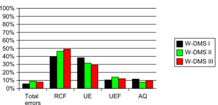
Figure5depicts the error rates for the three exper-iments. The overall amount of errors was moderately low, about 6–9% in all three experiments.8 About 40–
50% of these errors occurred in conjunction with a rule change (RCF) and ∼30–40% of the errors were clas-sified as “unmotivated errors.” The portion of errors categorized as “UEF” was comparatively low (about 10%) as was the portion of acquisition errors (AQ). These results show that perseverative errors constitute the greatest part of all of errors (RCF). However, the error data do not allow to draw definite conclusions with respect to the reason of unmotivated errors and a potential relationship of UE and UEFs. We further examined this item with the support of the neurody-namical simulations.
3.1.2 Simulations
The simulation results for four exemplary simulations using different fluctuation schemes are depicted in
Fig. 5 Average error rates and types as determined for WDMS I, II and III. Total errors: summary of all error types relative to the total amount of trials. The total errors are constituted by: RCF–errors in the context of a rule change, (Rule Change Follow up). UE–unmotivated errors , UEF–errors following a previously unmotivated error and AQ–acquisition errors
Fig. 6. For simulations number 1,2 and 4 the mini-mal response threshold was set to ”0”, for simulation number 3 we used the threshold Tmin=Tyes=Tno. Overall, the absolute response times (in ms) obtained in the simulations turned out to be lower compared to the experimental results, described above. However, the exact match of the quantitative results is considered to be of only minor importance as a constant factor is assumed to account for the explicit generation of subject motor responses and for further technical cir-cumstances (as the keyboard delay e.g.).
The stimulus congruency effects (Fig.6, left column) are qualitatively comparable to those obtained during the experiments for all four simulations: response times for “both” conditions are lower compared to response times for “match” conditions and “yes” responses are faster than “no” responses. The response time for “non-match” conditions is slightly increased compared to the response time for “none” conditions. Besides, the simulation using a minimal threshold (simulation 3) produced the inverse effect: The response time for the “none” condition was increased compared to the “non-match” condition similar to the numerical relationship of response times for WDMS III.
Response times relative to the set shift (Fig.6, mid-dle column) are moderately increased for the simula-tions 3 and 4, comparable to the experimental findings whereas for simulations 1 and 2 no set shift effect showed up.
The total error rates (Fig.6, right column, about 13% for simulations 1 and 3, 0.33% for simulation 2, and about 17% for simulation 4) are partly higher compared to experimental values but constituted to the largest extend by perseverative errors comparable to the ex-perimental results. The amount of unmotivated errors, however, appear to be lower for all four simulations compared to the experimental results.
3.1.3 Summary
Experiments as well as simulations revealed increased response times for incongruent compared to congru-ent trials comparable to the effects commonly ob-served with Stroop tasks (e.g. Gilbert and Shallice2002; Monsell2003). However, this item appears to be true only for congruent trials with “both” conditions but not for the trials with “none” conditions. For the sim-ulations, a striking effect turned out to be that he usage of the additional minimal threshold inverted the relationship between “none” and “nonmatch” trials.
These results raise two principal issues with respect to the experimental results:
(1) The error rates produced by the simulations are higher or lower than the average experimental values. Also, the simulations suggested so far a higher portion of perseverative errors than the av-erage experimental results. Do the experimental mean values constitute a “representative” exam-ple? Are individual significant variations possible and relevant?
(2) It is assumed that subjects memorize both stimu-lus dimensions during the trials and that, further on, the irrelevant stimulus dimension “supports” the response according to the relevant dimension in congruent trials. But why is this the case only for “both”-conditions and not as well for “none”-conditions? In other words if the response times for trials with “both” conditions are significantly faster than the response times for “match” condi-tions why is this not the case for “none” compared to “nonmatch”conditions?
The first question touches a very central point: Do the simulations cover individuals or an “averaged” in-dividual? What are legal limits for the simulations? The second question might touch a similar area: Are individual response time variations possible and poten-tially as well significant? The simulations hint at least at potential differences with respect to the threshold Tmin. Both items are investigated by analyzing subject based results to judge the expressiveness of the experi-mental mean values.
3.2 Individual performance measures
We analyze individual subject behavior during the ex-periments by considering response time distributions for the different match conditions as well as individual error rate and type variations.
Overall 15 simulations using different fluctuations schemes and model options served as a data base for the
Stimulus Set shift Error rates
Congruency Response Times and types
1
2
3
4
Fig. 6 Results obtained in four simulations of 300 sin-gle trials each with slightly varied parameter values and threshold sets. Simulation No. 3 used a minimal thresh-old Tmin=Tyes=Tno, for the remaining simulations Tmin=0
was used. Left: response times in dependence of the stim-ulus congruency. Middle: response times relative to the set shift; RC 1–first trial after the rule change, RC 2–second
trial afterwards, RC X–all other trials. Right: error rates and types elicited during the simulations; total errors–sum of all error types relative to the total amount of trials. The to-tal errors are constituted by: RCF–errors in the context of a rule change, (Rule Change Follow up). UE–unmotivated er-rors , UEF–erer-rors following a previously unmotivated error and AQ–acquisition errors
comparison with individual results. Simulations 1, 5 and 10 were conducted with controlled fluctuations for the remaining ones the external fluctuations were varied by different random seeds (further details regarding the model configuration are provided as supplemental material, Table5).
3.2.1 Stimulus congruency effects
For the analysis and comparison of individual response times the obtained mean values for the four differ-ent match conditions were normalized i.e. the smallest value was set to “1,” the remaining values to the re-spective relative amount. The same procedure was used
to compare the standard deviations for the different match conditions. As the relationship of the four match conditions is of central interest the normalization is a useful procedure to ease the comparison. Further on, the comparison of mean values and standard de-viations, as described in the following, enhances the overall expressiveness of the task model.
Subject response times An analysis of the normalized
mean response times and the standard deviations re-vealed that a majority of subjects form distinguishable “response groups” with striking characteristics (see Fig.7, left column).
Eighteen participants are subsumed to a response
group A. For this group the (normalized) mean
re-sponse times for “nonmatch”-trials were slower or equal to the response times for “none”-trials and the standard deviation turns out to be much smaller for “none”-trials compared to “nonmatch”- as well as “match”-trials. The mean values for this group (Fig.7, “Characteristics”) now reveals a significant9 though
small difference for the mean RT (-0.02) and a greater difference when comparing the standard deviations (-0.1) for “none” trials compared to “nonmatch” trials: – mean RT: t(17)= −2.39, p=0.029; difference
(none-nonmatch): -0.02
– mean RT stdv: t(17)= −3.58, p=0.0023; differ-ence (none-nonmatch): -0.1
For response group B, ten participants showed the slowest mean response times for “none”-trials as well as the largest standard deviations. Again significant effects for the relationship of “none” trials compared to “nonmatch” trials showed up:
– mean RT: t(9)=5.96, p=0.0002; difference (none-nonmatch): 0.08
– mean RT stdv: t(9)=3.13, p=0.012; difference (none-nonmatch): 0.17
It seems note worthy that the major differences between response groups A and B are constituted by response time variations, i.e. the standard deviations.
The remaining 12 participants (response group C) were neither assignable to response groups A or B nor showed any other groupable response behavior. However as more than 70% of the participants were subsumable to response groups A and B these groups are considered as the main focus for the simulations.
Simulation response times The simulations (Fig. 7, right column) allowed the reproduction of the response behavior of groups A and B via a very straight parameter set. For Tyes=Tno with Tmin=0 usually
x<<y is required (compare supplemental material).
This threshold configuration leads to model response times comparable to response group A. The only difference to the simulations covering response group B is the assumption of a minimal necessary response threshold for the model with Tyes=Tno=Tmin.
The explanation of this model behavior is compara-tively easy: For “no” responses the memory pool activ-ity is required to stay below a threshold y number of
9using paired students t-test
Fig. 7 Normalized response times for the different match con-ditions for the subjects (left column) and the simulations (right column). Simulation response times for response group C (bot-tom right diagram) are only shown for completeness and were beyond the scope of this work. For response groups A and B we see differentiable characteristics for the mean response times as well as for the standard deviations. For response group A the response time for “nonmatch” trials is higher than the response time for “none” trials whereas the “none” trials turn out to show comparatively low standard deviations. For response group B we see a high variation in the response time for “none” trials (higher stdv) and the mean response time for these trials is higher compared to “nonmatch” trials. These characteristics were reproduceable by the simulations (right column). Simulations using a minimal threshold (Tmin=0) elicited qualitatively theresponse time behavior of response group B whereas without this threshold (Tmin=0) mean response times and standard
deviations were qualitatively similar to the profile of response group A
times (with y comparatively large). Thus, the response times for the “none”-trials will not vary too much because the spiking rates of the neuronal pools first
decrease after the presentation of the test stimulus and increase again afterwards. Thus the model reaches the
“no”-response in the “none”-trials at a comparatively fixed point in time (determined by y). Indeed, the simulations show that the standard deviation tends to zero for “none”-trials which is as well an explanation for the comparatively large differences in the simulated standard deviations compared to smaller differences for the subjects.
The situation changes if a minimal threshold is required for task model responses. This minimal thresh-old provides the opportunity for response time
vari-ations in “none”-trials and leads as well to larger
response times in these cases.
Taken together, a possible explanation for the miss-ing significant effects when considermiss-ing experimental mean response times for the “none” compared to the “nonmatch” trials might be: Varying individual (neu-ronal) response algorithms superimposed each other. Thus, without the assumption of a minimal thresh-old the irrelevant stimulus dimension supports the response according to the relevant stimulus dimension in a similar way for “both” as well as for “none” conditions.
Besides the so far described simulation response times, a variety of other response time characteristics are possible when different thresholds for Tyes and
Tnoare used, with Tyes=Tno or x>> y for example. Figure7(right column, bottom diagram) shows exam-ple response times for Tyes=Tno. This item is depicted to illustrate that the task model provides the possi-bility to simulate further varying response behavior.
However, the current simulations do not cover subject response times in response group C and are considered to be subject for further investigations. We hypothe-sized that the response time distributions generated by
response group C might be the result of verbalization (or related) techniques used by the participants to en-hance the task performance which are beyond the scope of the present model.
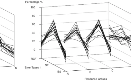
Fig. 8 Comparison of error types I and II. Left: comparison of standard error types (RCF, UE and UEF) for response groups A, B and C and the simulations (S) and average values (thick lines). Right: comparison of error types II for response groups A,
B and C and the simulations. RCF: errors occurring immediately after the valid rule was changed. SE: single errors. ES: sequences of two or more errors. Simulation no. 5 was excluded from this calculations as only one error occurred
3.2.2 Error rates and types
Further on, the relationship between perseverative er-rors and unmotivated erer-rors (RCF, UE and UEF) is investigated while leaving aside the consideration of acquisition errors (AQ) as they are first of all of only minor relevance and the simulations did not consist of multiple blocks. Figure 8, left diagram, shows the relationship of the remaining three error types for the response groups and the simulations. Most of the sub-jects across all response groups produced error rela-tionships similar to those elicited by the simulations: The amount of perseverative errors (RCF) is greater than the amount of unmotivated errors (UE), followed by the amount of UEFs.
However, none of the simulations showed error type distributions where the portion of unmotivated errors (UE) is greater than the portion of perseverative er-rors (RCF) contrary to numerous individuals across all response groups. But one-tailed t-tests (see as well sup-plemental material, Table8) revealed that the overall portion of RCFs is significantly higher than the portion of UEs at least for response groups A and B.10 This
circumstance first of all further supports the hypothesis generated by the simulations that subjects of response groups A and B should not show significant differences in error rates or types. Further on, it is hypothesized that the comparatively high amount of unmotivated
10Difference between rate of RCF and UE = 15% for response
group A and 12% for response group B, ( p=0.0005, respectively, p=0.01).
errors committed by several individuals might be rea-soned in the usage of higher cognitive processes beyond the scope of a neuronal model (subjects might have tried unsuccessfully to use a new rule during the main-tenance phases or were otherwise distracted during the experiment).11 Thus in summary, we might state that
the simulations elicit reasonable error rate and type distributions providing even the potential to exactly match individual behavioral variations.
When considering now the context of errors elicited during the simulations we are able to detect the follow-ing dependencies:
If a rule change after the provision of the negative feedback succeeded the new valid rule is quite reliably established already in the following trial.12Thus, a true perseverative error (RCF) might more likely be defined as an error occurring immediately after the provision of the negative feedback.13 This implies that a new rule
is considered to be established already with the first correct answer after the set shift.
Additionally, the simulations suggest a distinction between single attentional errors and sequences of errors occurring during the maintenance phase of an
11Single errors due to expected “chance hits” were as well
as-sumed by Nakahara et al. (2002)
12Compare for example Fig.2, supplemental material, trials 89
and 96.
established rule. For a single (attentional) error the simulations suggest two possible reasons:
(1) An arbitrary rule change.14
(2) A fuzzy development of the ssr. This means that the memory pool activity (ssr) is not clearly as-sociated to either a “yes” or a “no” response which leads to a wrong model answer but not to a change of the active rule after the provision of the negative feedback due to a lack of sufficient activ-ity difference or, again, external fluctuations.15A
behavioral translation for this behavior would be reduced attention leading to a reduced differentia-tion of relevant and irrelevant stimulus dimension. In both cases these single errors are reasoned in fluctuation in the external AMPA input. The degree of these fluctuations might well be translated into a degree of “attention” a participant pays to the current experiment. If participants do not attend the stimulus display properly they enter into a response conflict because the relevant stimulus dimension is not “strong” enough to provide the base for a definite answer.
Additionally and on contrary, the simulations show sequences of errors following an initial attentional er-ror similar to RCFs and indicating again persevera-tion. From the model point of view, “perseveration” is marked by the inability to switch to a new rule after the provision of a negative feedback.
Thus, for analyzation purposes the error types were redefined as follows:
Error Types II
Rule change errors (RCE): These are necessary
er-rors subjects make (in the rule change trial) when the valid rule is changed without notice (same definitions as before, see Fig. 1, bottom, trial 2).
Errors in the context of a rule change (RCF): These
are errors occurring immediately after the valid rule was changed. They follow immediately after the nec-essary RCE of a previous rule change.
Single errors (SE): These are single errors made in
the maintenance phase of a specific rule. The previ-ous and following trial has a correct answer.
Error Sequences (ES): Errors occurring in a series of
two or more errors during the maintenance phase of a specific rule.
14Figure2, trial 100, supplemental material. 15Figure3, trial 98, supplemental material.
The major questions when analyzing these error types II is whether they occur to the same extend in the simulations and the experimental data and thus further support the plausibility of the task model.
Figure 8, right diagram shows the relationship of error types II for the response groups and the sim-ulations. Across all three response groups single er-rors comprise the greatest part with only individual exceptions: In every response group one participant produced a greater amount of error sequences than single errors. The simulations show very similar error profiles: Five simulations (no. 3, 11, 12, 14 and 15) led to an error profile where the amount of single errors is greater than the amount of error sequences. Further seven simulations (no. 1, 6 to 10 and 13) produced error profiles similar to those of the “exceptionists” within the response groups; and only two simulations (no. 2 and 4) produced error profiles where the amount of sin-gle errors constituted the smallest part. These last two profiles are not represented amongst the participants of the WDMS experiments.
3.2.3 Summary
The response times achieved during the simulations indicated that all model options are able to account for the corresponding individual results with the mini-mal threshold (Tmin) explaining a major differentiation criteria (response groups A and B). Further more it is hypothesized that verbalization techniques used by the participants are reflected in response time distributions deviant from these profiles (response group C).
Similar, several error profiles were detectable amongst the experimental participants as well as the simulations and only two out of 15 simulations pro-duced an error profile which was not represented amongst the experimental participants.
The aim to match experimental mean values
ex-actly would require to select a set of simulations that
match the individual characteristics of the participants. However, so far we considered it highly satisfying to have demonstrated successfully that individual re-sponse variations are possible and relevant within an experimental design and that it is possible to suggest neuronal correlates which are able to account for these differences.
4 Discussion
In this work we presented a biophysical detailed neu-rodynamical model for a delayed-match-to-sample task
with a Wisconsin-like paradigm (WDMS experiment). The experimental design combined several elements: – DMS elements: The primary task required to
com-pare a sample stimulus with a test stimulus, pre-sented after a delay period.
– Stroop elements: Different match conditions of sample and test stimulus resulted in trials with con-gruent and inconcon-gruent conditions.
– Wisconsin elements: The valid rule was not explic-itly informed. Participants were required to detect the valid rule based on provided feedback. The valid rule was switched without notification at ar-bitrary intervals.
The WDMS experiments were conducted with 40 healthy participants. Key experimental results turned out to be:
– Increased response times for incongruent com-pared to congruent match conditions with “yes” responses being faster than “no” responses. – Individually varying response profiles especially
with respect to “none” conditions.
– Moderate error rates with different types of errors related to the perseveration of the previous rule and further attentional errors.
The experimental results were reproduced by a vari-ety of simulations using a biophysically detailed neuro-dynamical model. The design of the model was oriented on neurophysiological findings and used an asymmetric set of weights to accomplish the set shift. The errors committed by the model during the simulations were related to system inherent fluctuations in the input of other cortical areas to the explicit model neurons. The degree of these fluctuations is translateable into the degree of a participants attention: The higher the atten-tion the smaller the error rates. Hence the fluctuaatten-tion effects represent an explanation for errors committed by healthy subjects in this experiment and did not require any additional handling (as feedback delay, see Rougier and O’Reilly2002; Rougier et al. 2005). Fur-ther more, the simulations suggested an explanation (in terms of different response thresholds) why response times for incongruent trials are slower than those for congruent trials and why this relationship differs for “none” trials.
The overall operation of the model illustrated how abstract rules (i.e. “selective attention”) might oper-ate to influence and amplify task-relevant information rather than suppress task-irrelevant information, a cir-cumstance which was recently confirmed by Egner and Hirsch (2005). The active neuronal rule does not inhibit
the irrelevant feature dimension but supports the rele-vant feature dimension to a slightly higher extend.
The experimental results revealed that subjects do produce single attentional errors and are at the same time able to switch the valid rule with a single error trial in this WDMS set shifting task, a question opened in Section 1. The neurodynamical model was able to suggest explanations for these attentional errors. Al-though the WDMS task uses only tow different rules opposed to the classical “Wisconsin Card Sorting Test” modeled by Rougier and O’Reilly (2002) and Rougier et al. (2005) it is very likely that the findings presented in this work apply to the WCST to the same extend.
In this respect a central question concerns the ap-plicability of the suggested asymmetric weight set for tasks using three different rules, and whether such an approach would be capable to solve the problems of existing models as depicted in Section1.
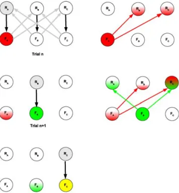
Figure9illustrates this principal possibility and ex-tends Fig.3for a three-rule-setup. We explore the time course of input provided by the memory pools to the rule pools within three successive trials (n, n+1, n+2). For simplification, we consider only one memory pool per rule pool. The first diagram shows the principal task model including the strongest weights (black and gray arrows for feedforward, respectively, feedback connec-tions) compared to the remaining ones (not shown).
Fig. 9 Schematic extension of the memory based switching algo-rithm for tasks incorporating three rules and exploration of the input dynamics
Rule pool RAand memory pool FAare assumed to be active. Further, we assume a set shift after trial n and the according destabilization of the rule pool activity. Hence memory pool FAwill provide the strongest input to the rule pools RBand RC(second diagram). Thus, rule pools RB and RC will enter into a competition. Under the assumption that RBwon this competition we will see a spiking activity scheme as depicted for trial
n+1. We also assume that memory pool FAstill shows some degree of activity in line with the principal feature amplification strategy for set shifting tasks (e.g. Egner and Hirsch2005). Also, it might be assumed that the pool FAshows still some amount of activity due to its relevance in the previous trial. Details about the degree of memory pool activity remain to be investigated in corresponding experiments. As RB was not the right choice a further negative feedback will be provided following trial n+1. The fourth diagram now illustrates that pool RC receives the greatest amount of input from the memory pools and thus will be the active rule pool in trial n+2with a high probability. Again, the stimulus memorization will depend on the degree of external fluctuations (reflecting participant attention) as for the two-rule WDMS task model. Hence, there is only a high probability for the model to choose an optimal search procedure for a new rule leaving room for the production of realistic error profiles opposed to the models described in Section1.
For the further investigation of patient behavior with the WDMS the suggested neurodynamical model offers promising analyzation perspectives. First of all, if neg-ative feedback signals are not provided to a sufficient extend a switch of valid rules would be impossible. Thus a “restart” of the task would be necessary to enable the possibility to select a different rule. An interrupt leading to a task restart might be generated by (controlled) external distractors in an experimental paradigm. Such external distraction would account as well for a comparatively low amount of “unmotivated errors.” Perseverations due to disturbed feedback sig-nals are probably related to the task performance of patients suffering from Parkinsons disease who did not show a pattern of increased distractibility.
Secondly, if the entire or part of the rule pools are missing a similar behavior is possible. I.e. an once se-lected stimulus dimension is not changed except due to external distractions leading to a “task restart.” Missing rule pools would constitute as well an explanation for the two phenomena observed with prefrontal patients: Increased perseveration and distractibility. The per-severation arises from the circumstance that there is actually no rule to select and hence no feature
ampli-fication possible. But visual information processes still
ensure the ability to recognize just one of the features. The distractibility arises from the circumstance that, accordingly, there is no rule to maintain. Further on, without feature amplification the irrelevant stimulus dimension is most probably ignored. Thus, the differ-ences between the response times for congruent and incongruent trials would disappear. The patient be-havior related to these phenomena might be classified by “perseveration and distractibility” and both aspects together are supposed to constitute the reason for per-formance deficits of prefrontal patients.
Thirdly, the simulations revealed a major effect of the fluctuations in the external AMPA input on the response accuracy. Thus, “fuzzy” memory pool activity might be increased by an increase in these fluctuations, whereas its limitation should lead to increased response accuracy. The major effect of increased fluctuations is proposed to be an high amount of single errors (due to a “fuzzy” ssr) and potentially as well a slight increase in perseverative errors immediately after an rule change as the switching procedure is rather sensitive to these fluctuations. The patient behavior related to these phe-nomena might be classified by “attentional deficits.”
As a last issue, a reduced level of glutamate is sug-gested16 to limit the working memory capacity which
leads to a strong increase of all error types.17Further on, response time differences for congruent and incon-gruent trials disappear as at least the irrelevant stimulus feature is not maintained across the delay periods. Also, the overall performance of the task will strongly depend on the duration of the delay period. The patient behav-ior related to these phenomena might be classified by “a working memory deficit.”
Attentional deficits and/or working memory deficits might thereby account for the (divergent) task perfor-mances observed with Schizophrenic patients.
A final remark might be appropriate with respect to the modeling level chosen in this work. The usage of a biophysical detailed model comprising “Integrate-and-Fire” neurons for the simulation of set shifting tasks proved so far to be highly useful. However, it is well possible to (a) incorporate even more neuronal details (e.g. Hodgkin and Huxley 1952; Meunier and Segev
2002), or (b) to vary the homogeneity of the neurons used in this approach (for example by a heteroge-neous neuronal configuration and connectivity) or (c)
16Based on rough example simulations using a 10% reduced level
of glutamate. Similar to the study of Durstewitz and Seamans (2002).
17Though in this case, the errors are not of a perseverative
“nature” but only appear to be perseverative. If stimulus features are not memorized according errors cannot be perseverative.