and Optimal
Consumption-FAME - International Center for Financial Asset Management and Engineering
40, Bd. du Pont d’Arve PO Box, 1211 Geneva 4 Switzerland Tel +41(0)22 312 09 61 Fax +41(0)22 312 10 26 www.fame.ch admin@fame.ch February 2003 Research Paper N° 104
Andriy DEMCHUK
HEC-University of Lausanne and FAME
Sovereign Debt Contract
Investment Strategies
Sovereign Debt Contract and Optimal
Consumption-Investment Strategies
∗
Andriy Demchuk
University of Lausanne and FAME
Abstract
We present a model in which a sovereign country optimally decides on its consumption and investment policies as well as on the optimal time to default. In the paper we allow the sovereign borrower to keep the fraction of its augmented wealth in so-called international reserves. We further assume that these reserves can be deposited at the risk-free rate. In this framework, we obtain analytical solutions for optimal consumption and investment rules, as well as formulas for optimal default boundary and the value of the risky loan. In the paper we assume that in the case of default the lender can impose economic and political sanctions against the borrower and also can seize an implicit collateral. We show that when the country is getting very close to its default wealth level, then its relative risk aversion decreases and the country increases its consumption rate and the risky investment fraction at the expense of available liquid reserves.
Keywords: sovereign debt, international reserves, strategic default JEL ClassiÞcation: C61, G11, G13
∗I am grateful to professor Rajna Gibson for her comments and suggestions. I also would like to thank Ren´e Stulz, Ernst-Ludwig von Thadden, the participants of FAME PhD workshops and session participants at the European Envestment Review Meeting for comments and useful discussions. I gratefully acknowledge the support of the Training Center for Investment Professionals (TCIP), Switzerland.
(E-mail: ad@fame.ch)
1
Introduction
Sovereign countries may apply for external Þnancing for different reasons. Some of them may want to expend the scale of the investment in projects or technologies they are already running or going to undertake or estab-lish. Others may need extra funds to cover their budget deÞcit, that is for consumption. We construct a model in which the sovereign borrower en-dogenously derives his optimal consumption and investment policies. Our model is based on a key assumption that the country not only consumes and invests in the risky technology, but also keeps a fraction of its wealth in so-called international reserves. These reserves are created for consumption smoothing purposes and, by assumption, can be invested or deposited at the risk-free rate. This assumption makes our model conceptually different from other studies - in fact we allow for the existence and optimal management of international reserves.
Under this assumption we study the behavior of the sovereign borrower who has only one single borrowing opportunity. That is, we do not allow for repeated borrowing in our model, and we consider a static debt contract. This implies that the borrower gets more discretion over the way he spends borrowed funds since the reputation effect vanishes. When a debt contract is signed, the sovereign country decides upon its consumption and investment policies and the time of default without any possibilities for the lender to interfere. However, in order to sustain positive lending, we assume that if the borrower defaults, the lender can impose economic and political sanctions and can seize a fraction of borrower’s assets.
The above assumptions, among few others, are widely used in the liter-ature on sovereign lending. The idea is that there must be some incentives for the sovereign country, which can hide behind its sovereignty, to respect the debt service. If a country decides to default, and hence refuses to pay a contractual coupon, then costly and lengthy renegotiations usually take place since there is no well establish bankruptcy procedure. This is the main difference between a sovereign and a corporate debt contract. The latter is an enforceable contract due to the presence of the bankruptcy code, for in-stance Chapter 11 in the USA. If a corporation fails on its debt obligations, then the bankruptcy procedure is well deÞned and the lender can have access to the assets of the borrower.
In sovereign debt models, the partial access to the assets of the defaulted borrower is usually taken by assumption. In reality, however, it can be quite problematic and costly for the lender to seize borrower’s assets and transform them into cash. The parties rather begin to negotiate over the
strategic debt service or partial debt relief. In the paper, we also allow the parties to negotiate when the sovereign borrower fails to provide the contractual coupon payment.
Our model is much in line with one of Chang and Sundaresan (2000). In their paper, a sovereign country uses its wealth for consumption purposes and investment in its risky technology. When maximizing the expected util-ity from life-time consumption, a country endogenously decides upon the default boundary as well as upon the re-borrowing boundary. The authors also derive the differential equation the value a risky loan must satisfy. How-ever, in their model all the results are numerical ones.
The major difference between our study and the one of Chang and Sun-daresan is driven by the risk free lending opportunity for the borrower in our model. Even though their model allows for the dynamic borrowing, it does not seem problematic to extend our model to the dynamic setting by using the technique of Chang and Sundaresan (2000). Interestingly, in our framework the sovereign country is in the role of a risky borrower and a risk-free lender simultaneously. The introduction of the possibility for the sovereign country to manage its reserves allows us to derive explicit and im-plicit analytical solutions for the value function, optimal consumption and investment rules, the default boundary and the value of the risky loan.
The rest of the paper is organized as follows: In section 2, we provide a brief literature review. In section 3, we present the setup of the model were we basically describe the rationale for the country to become a borrower and a lender simultaneously. We also present there the timing of the model. In section 4, we solve the borrower’s optimization problem before he defaults and also during the renegotiation period. In section 5, the value of the risky loan as well as the contractual coupon value are derived. Section 6 presents some numerical results and section 7 concludes the paper.
2
Literature overview
Many studies have addressed the issue of the sovereign lending from different perspectives. Very generally, there are two approaches in the literature to study the rationale for sovereign lending or borrowing.
TheÞrst approach is based on the assumption that a sovereign borrower values his reputation if he wants to have an access to the credit market in the future. Models which deal with this approach assume that the borrower who once defaults is unable to enter into anotherÞnancial agreement. Eaton and Gersovitz (1981) build a reputation based model to explain the rationale for
sovereign lending. They consider a sovereign borrower who maximizes utility from consumption and uses external funds to share the risk of his domestic production technology. In their model, it is assumed that default leads to the exclusion of the borrower from the world credit market. The authors show that under certain conditions reputation effect allows for positive lending equilibrium. However, Bulow and Rogoff (1989b) argue that if cutting off future loans is the lender’s sole threat, then there is no lending equilibrium if the borrower is able to enter cash-in-advance agreements.
The second approach considers economic and political sanctions as a main threat of the lender in the case of default. Bulow and Rogoff(1989a) consider economic and political sanctions which may be imposed by the lender as an instrument to achieve a positive lending equilibrium. Gibson and Sundaresan (2000) model penalties as a seizure of the borrower’s exports combined with economic sanctions. They assume that borrowings are used to generate exports, which in turn will partially serve as a collateral. In our paper, we make the same assumptions about sanctions and seize of collateral as main instruments to hurt the defaulted borrower, but we do not model exports explicitly.
Chang and Sundaresan (2000) present a continuous time model which allows for repeated borrowing and sanctions. In their paper, default is fol-lowed by renegotiations during which the borrower pays a strategic coupon. Renegotiations last until the borrower recovers from the distress and resumes to pay a contractual coupon or until the lenders unilaterally terminates ne-gotiations. The latter happens at the low wealth level of the borrower when the strategic coupon which the lender receives is equal to his bargaining cost. Chang and Sundaresan also indicate under which circumstances the sovereign country will be willing to re-borrow. In the paper they derive the optimal default boundary as well as the optimal re-borrowing boundary. In our paper, we use a framework of Chang and Sundaresan, but we do not model re-borrowing opportunities. Instead, we allow the sovereign country to keep a fraction of its wealth in the international reserves.
There are a few studies which address the issue of sovereign credit spread estimation. Gibson and Sundaresan (2000) show that in the framework of their model sovereign credit spreads are strictly grater than spreads of an otherwise identical corporate debt contract. They obtain that both sovereign and corporate credit spreads are increasing convex functions of the coupon rate and inversely related to the level of the risk-free rate. Westphalen (2001) presents a Þnite horizon continuous time model of rescheduling of debt following a sovereign default as a bond exchange. He obtains, as we do, closed form solutions for the default boundary, the value of the bond
and credit spreads.
Duffie, Pedersen and Singleton (2003) construct a reduced form model for pricing sovereign debt and estimate the model using Russian dollar-denominated bonds. Along with credit spreads estimation, the authors study the determinants of Russian yield spreads which are: budget deÞcit, current account, reserves of hard currency and the required future debt ser-vice. One of their major Þndings indicates that Russian yield spreads are negatively correlated with the country’s foreign currency reserves and the oil price. Our model is able to explain this empirical fact when the country is close to its default boundary: credit spreads move up and the level of the country’s international reserves decreases substantially because of increased probability of strategic default.
3
The setup of the model
We consider a production type economy in which there is one single good which serves as a numeraire and which is used for consumption and invest-ment purposes by all agents in the economy. Thus, consumption and wealth are measured in units of the numeraire.
We study the interaction between a representative lender and the bor-rower with initial wealth x0. In our model this particular borrower is a
”small” (in a sense of wealth) sovereign country which cannot affect the world risk-free rate. This interaction takes place in a full information set-ting, i.e. the lender knows (or can perfectly monitor) all the characteristics (actions) of the borrower, and vice-versa.
The sovereign borrower seeks to augment his initial endowment x0 by
applying for externalÞnancing. Whether the borrowing takes place or not, the borrower is assumed to use his wealth for consumption purposes (for instance to service the country’s budget) and for investments. To keep things simple, we assume that investment opportunities are restricted by only two technologies.
The Þrst one is the borrower’s own (or domestic) risky production tech-nology an investments of qt in which instantaneously yields:
dqt
qt =µdt+σdZt
where µand σ are the instantaneous return and its standard deviation re-spectively, both are positive constants. Zt is a standard Brownian Motion on the underlying probability space (Ω,F,P) which describes all the un-certainty in the production process. This risky technology models a total
country’s stock and it incorporates all the production the government of a sovereign is managing or is responsible for, including the production of export oriented products.
The second investment technology constitutes the possibility for the sovereign borrower to lend at the risk-free rate. The assumption about the existence of this riskless investment opportunity drives a wedge between our study and the one of Chang and Sundaresan (2000). By introducing the second technology, we simply assume the following. Apart from consump-tion and investment in the risky technology, the sovereign borrower keeps a fraction of his wealth in ”reserves” for consumption smoothing purposes. This can reßect, for instance, liquid international reserves of the country’s National Bank. As an example, in Table 1 we present statisticalÞgures for gross international reserves of the Russian Federation for years 1996-2001. As it is indicated, the foreign exchange assets constitute the major part of the country’s international reserves. Also, these assets accounted for 2.7% in 1996 and nearly 11% in 2001 of the country’s GDP. Moreover, from the deÞnition of the foreign exchange assets, it makes sense to consider their default risk as negligible. Therefore, we assume that liquid international reserves of the sovereign borrower yield a constant risk-free rater,such that r < µ.In our model, optimal consumption, optimal investment in the risky technology as well as the optimal size of the borrower’s international reserves will be derived endogenously.
At time 0, the sovereign country considers the possibility to augment its initial wealth. Suppose that it has incentives to borrow from abroad by signing a debt contract of the form (I∗,C(I¯ ∗))1, where I∗ is the amount borrowed and ¯C is the corresponding coupon. In the paper we consider a perpetual debt contract, i.e. there is no repayment of the principal amount of the loan, but the borrower commits to pay to the lender a perpetual continuous couponßow ¯C(I∗),where the value of ¯C(I∗) is deÞned endoge-nously in our model. We also assume that this borrowing technology is static, i.e. the borrower can augment his wealth via externalÞnancing only once. Therefore, after the debt contract (I∗,C(I¯ ∗)) is signed, the notion of ”reputation” vanishes for the borrower. We also assume that the initial wealth of the sovereign country is not that high that it can be treated as a ”safe” borrower. Hence, the debt contract we just described encounters credit risk and the initial yield of the loan must be above the risk-free rate r.
1
The country’s insentive to sign such a countract will be formalized in Assumption 1 in section 4.
Table 1. Gross International Reserves of the Russian Federation2 (in billions of US$) GDP Gold and foreign of which
(nominal) exchange reserves foreign exchange assets Gold
(% of GDP) 31.12.1996 419.0 15.3 11.3 2.7% 4.0 31.12 1997 436.0 17.8 12.8 2.9% 4.9 31.12.1998 282.4 12.2 7.8 2.8% 4.4 31.12.1999 193.2 12.5 8.5 4.4% 4.0 31.12.2000 251.1 28.0 24.3 9.7% 3.7 31.12.2001 302.2 36.6 32.5 10.8% 4.1
Sources: The Central Bank of Russian Federation, Datastream
If at a certain point of time the borrower is unable or unwilling to respect the contractual coupon payment of ¯C, we will call this event as default. If this event occurs, following Bulow and Rogoff (1989a), Gibson and Sun-daresan (2000) we assume that the lender can penalize the country in the following ways:
First, the lender can impose political or economic sanctions against the borrower, which in turn will result in the future reduction of the borrower’s risky technology growth rate from µ to ˆµ3, µ < µ.ˆ For example, if the borrower’s production heavily relies on some particular import products (like energy resources, raw materials, etc.), the lender may have the possibility to inßuence the supply side of these products, and hence to hurt the borrower. The lender may also have the possibility to impose some trade barriers such that the borrower’s exports, and thus revenues, will diminish.
Second, the lender can seize some assets of the borrower. Namely, the lender can expropriate a fraction β of the borrower’s wealth at the time of default. One could think that via a certain legal procedure (like a trial in an international court) the lender can get an access to the borrower’s as-sets abroad, for instance borrower’s exports, like in Gibson and Sundaresan (2000), or some other tangible assets. However, we assume that the lender cannot get an access to the international reserves of the borrower when the
2
The international reserves are highly liquidÞnancial assets that the Bank of Russia and Ministry of Finance have at their disposal on the reporting date. The international reserves are made up of monetary gold, special drawing rights (SDR), reserve position at the IMF and foreign exchange assets. The foreign exchange assetsincludes the Bank of Russias and Ministry of Finances foreign exchange assets in the form of cash, reverse repo with nonresidents, bank deposits at nonresident banks (having not less than A rating by the classiÞcation of the Fitch IBCA and Standard and Poors or A2 by the classiÞcation of the Moodys) as well as government and other securities issued by nonresidents with a similar rating. Starting from September 1, 1999, a sum equivalent to the balances in foreign currency on the correspondent accounts of resident banks in the Bank of Russia is deducted from the above assets except the funds allocated by the Bank of Russia to the Vneshekonombank for servicing the government foreign debt.
borrower defaults4. Therefore, the borrower is aware that when he defaults, the fraction β (0< β < 1) of his wealth can be lost. Hence, by signing a debt contract, the lender receives an implicit collateral.
The wealth level W∗ at which the sovereign country decides to default
will be derived endogenously. Namely, at this wealth level the borrower becomes indifferent between continuing to service debt, i.e. to pay coupon
¯
C,and defaulting. In the paper, we assume that after default the sovereign borrower and the lender negotiate over the strategic debt service or, in other words, over strategic coupon ßow. In general, the outcome of such kind of negotiations depends on the bargaining power of the parties. On the contrary to Chang and Sundaresan (2000), in our paper we assume that the lender does not hold all the bargaining power during the renegotiations, but he can rather extract only a fraction α < 1 of the maximum coupon Smax(W) the borrower can pay at his wealth levelW. The maximal coupon Smax(W) lies on the boundary when the borrower is indifferent between paying this coupon and paying nothing (but accepting penalties). Since the reputation has no value for the country, the sovereign borrower will not enter renegotiations ifα= 1,i.e. when the lender has all the bargaining power. In Chang and Sundaresan (2000) the sovereign country is willing to negotiate under the latter condition, because in their model the country values future re-borrowing opportunities.
We denote the strategic coupon the borrower pays during the renegoti-ation period byS(W),and by assumption it is equal to5:
S(W) =αSmax(W).
Therefore, during renegotiations, the lender receives a strategic coupon S(W),and the amount
Smax(W)−S(W) = (1−α)Smax(W)
is left for the borrower in order for him to continue negotiations. In our model, the bargaining power parameter α is set exogenously, however it must be sufficiently high for the lender to have incentives to enter renego-tiation rather than ”liquidate” the borrower atW∗.The maximum coupon Smax(W) the borrower can pay during the renegotiation period will be de-rived endogenously. We also assume that negotiations are costly for the
4As our numerical solutions indicate, this assumption is not very restrictive because
the volume of international reserves approaches zero when the country is very close to default
5
Chang and Sunsaresan (2000) assume that the lender holds all the bargaining power during the renegotiations, and thus in their modelS(W) =Smax(W).
lender and he bears a bargaining cost ofbc per unit of time. In our model renegotiations end when either the country recovers from theÞnancial dis-tress and resumes to pay the contractual coupon ¯C, or the borrower’s econ-omy experiences series of negative shocks and his wealth reaches the point W∗ when the net cash inßow to the lender (S(W∗)−bc) becomes equal to zero. In the latter case, the lender unilaterally triggers sanctions and seizes the collateral. We call the corresponding event as total default and derive the trigger wealth levelW∗ endogenously.
In Table 2 we summarize the setup of the model.
Table 2. Region (or period) Corresponding borrower’s wealth Borrower’s wealth at the beginning of the period Growth rate of the borrower’s technology Debt service Continuation W > W∗ x0+I∗ µ C¯ Renegotiation W∗ < W < W∗ W∗ µ S(W) Total default W < W∗ (1−β)W∗ µˆ 0
Now, we specify the characteristics and the optimization problem of the sovereign borrower.
4
The borrower’s optimization problem
We consider a sovereign country with a power utility function derived from consumption:
U(c) = c
1−γ
1−γ, γ>1
After the debt contract (I∗,C(I¯ ∗)) is signed, the augmented wealth of the sovereign becomes equal tox0+I∗.It is assumed that from this point on the
lender has no possibilities to inßuence or intervene the actions the borrower undertakes, unless the latter defaults.
Therefore, the borrower solves his consumption-investment problem and strategically decides on the time, or equivalently on the wealth level, of default. At time 0, the value function of the sovereign can be written as:
J(x0+I∗) = Max W∗,(ct,wt)∈A E0 Z ∞ 0 e−ρtU(ct)dt (1)
where the controls c, w, and W∗ denote consumption, the fraction of the wealth to be invested in the risky technology and the optimal default bound-ary (i.e. the wealth level at which the sovereign defaults), respectively;ρis the subjective discount factor. A is a set of admissible controls:
A={(ct, wt) :ct≥0∧wt∈[0,1] ∀t≥0}
This optimization problem implies that at each point of timetthe frac-tion (1−wt) of borrower’s current wealth to be kept in reserves is derived6. By assumption, the reserves are invested at the risk-free rate. We should notice that this riskless investment is restricted: a) by the country’s current wealth from above, that is the short selling of the risky production technol-ogy is not allowed, and b) by zero from below, that is the sovereign cannot borrow money at the risk-free rate due to its default risk.
To proceed further, we make the following assumptions about the initial wealth and theÞnancial parameters of the model.
Assumption 1. In order for a positive debt contract (I∗,C(I¯ ∗)) to exist, we assume that, given the initial wealth of the sovereign country x0,
theÞnancial parameters of the model and the borrowed amountI∗ are such
that
a) the sovereign country has incentives to borrow, i.e. J(x0+I∗)> J0(x0)
whereJ0 is the country’s value function in autarky.
b) the lender has incentives to lend: x0+I∗ > W∗
The above inequality requires for the augmented wealth to be above the de-fault boundary. In other words, this condition precludes immediate dede-fault.
Assumption 2. Financial parameters µ, r,σ and γ are such that the risk-free investment is feasible for the borrower at any wealth level. Namely, we assume that7 0< 1
γ
µ−r
σ2 <1. 6
Notice that according to our deÞnition of the admissible strategy, this fraction can become very small, whereas a country’s central bank may be forced to fulÞl a certain minimum requirement on the level of international reserves. However, the incorporation of this constraint will not allow us to solve the model analytically.
7
This assumption will supports the existence of interior optima when we solve the borrower’s optimization problem.
To solve the borrower’s optimization problem (1), we proceed in the fol-lowing way. First, we consider the problem the sovereign borrower is facing when he totally defaults. Since there are no future borrowing possibilities, this problem is equivalent to the one when the borrower stays in autarky. Then, we formulate the initial optimization problem and the one during the negotiation period.
4.1
The sub-problem after total default
When wealth of the sovereign country reaches the total default boundary W∗, the lender imposes economic and political sanctions, which result in the reduction of the economy’s growth rate from µ to ˆµ, and seizes im-plicit collateral which is worth βW∗. In this case, the sovereign solves its consumption-investment problem with the corresponding value function:
ˆ J(W∗) = Max (c,w)∈AE Z ∞ 0 e−ρtU(ct)dt (2) and the wealth dynamics:
dWt = [(wt(ˆµ−r) +r)Wt−ct]dt+wtσWtdZt, t >0 (3) W(0) = (1−β)W∗
From the theory of dynamic programming it follows that given the wealth dynamics (3), the value function (2) satisÞes the following HJB equation8:
0 = max c,w {U(c)−ρ ˆ J+ ˆJW[(w(ˆµ−r) +r)W −c] + 1 2JˆW W σ 2w2W2 } (4) The explicit analytical solution to the above equation gives the formula for the value function as well as for optimal consumption and investment rules after total default:
ˆ J(W) = ˆδ−γW 1−γ 1−γ (5) ˆ c∗(W) = ( ˆJW)− 1 γ = ˆδW ˆ w∗ = − ˆ JW ˆ JW W W ˆ µ−r σ2 = 1 γ ˆ µ−r σ2
where ˆδ = 1γ[ρ+ (γ −1)(r + 21γ(µˆ−σr)2)]. Note that both ˆc∗ and ˆw∗ are admissible: ˆc∗ ≥0 because ˆδ >09,and ˆw∗∈(0,1) because of Assumption 2
8This equation is obtained by the application of the stochastic dynamic programming
technique (see, for example Fleming and Rishel (1975)). For details on the derivation of this HJB equation, see, for example, Merton (1971, 1990).
and the fact thatr <µ < µ. We can see that after total default, the optimalˆ consumption and investment rules of the borrower, given that he will not be able to borrow in the future, coincide with the classical Merton’s (1971) solution: the borrower consumes at a constant rate ˆδ and invests a constant fraction (often called as Merton’s rate) of his current wealth in the risky technology. He keeps the rest in international reserves and invests them at the risk-free rate by assumption.
Let us notice that equation (5) also gives a formula for the country’s value function at time 0 when it stays in autarky:
J0(W) =δ−γ
W1−γ
1−γ (6)
whereδ= γ1[ρ+ (γ−1)(r+21γ(µ−σr)2].
4.2
The initial optimization problem
Now, having deÞned the value function of the borrower after total default, his initial value functionJ(W) can be written as:
J(W) = Max W∗,(c,w)∈AE 0"Z τ ∗ 0 e−ρtU(ct)dt+e−ρτ∗J˜(W∗) # (7) where W∗ is the default boundary and τ∗ is the corresponding stopping time. ˜J(W) is the value function of the borrower during the renegotiation period.
In the solvency region, i.e. whenW > W∗,the borrower’s wealth evolves as:
dW(t) = £(w(µ−r) +r)W(t)−ct−C¯
¤
dt+wσW(t)dZt, t <τ∗ (8) W(0) = x0+I∗
where ¯C is a contractual coupon ßow. In this section we treat it as exoge-nously given, but in the next section we derive its value endogeexoge-nously, i.e.
¯
C= ¯C(I∗).
We assert that the sovereign borrower’s value function (7), given the wealth dynamics (8), is the unique C2(W∗,∞) solution of the following HJB equation10: 0 = max c,w {U(c) +JW[(w(µ−r)W−c] + 1 2JW Wσ 2w2W2 }−ρJ+ (rW −C)J¯ W (9)
with boundary and initial conditions: J(W∗) = ˜J(W∗) (9.1) lim W→W∗+ dJ(W∗) dW = dJ˜ dW(W ∗) (9.2) lim W→∞J(W) = limW→∞J0(W) = 0 (9.3)
Problem (9)-(9.3) is a free boundary problem which simultaneously yields the solution for the value function J and the default boundary W∗. The boundary condition (9.1) is a value matching condition which says that at the default boundary the borrower is indifferent between continuing to ser-vice debt with coupon ¯C and entering into renegotiations. Equation (9.2) is a smooth-pasting condition which ensures the optimality of the default boundaryW∗. Moreover, this condition also ensures continuity of consump-tion at the default boundary (we will consider this problem below in more details). The last condition (9.3) describes the asymptotic property of the value function: when the wealth of the country tends to inÞnity, then de-fault probability tends to zero, and hence the country behaves like being in autarky11.
Assuming that interior optima in equation (9) exist12, we use the Þ rst-order condition with respect to the risky investment fractionw:
w=− JW JW WW λ σ whereλ= µ−r σ (10)
Substituting (10) into (9) we get
ρJ =−1 2λ 2 JW2 JW W + (rW −C)JW¯ + max c {U(c)−cJW} (11) Now we use the Þrst-order condition with respect to consumptionc:
JW =U0(c) =U0(c(W)) (12)
11When wealth approaches inÞnity, the relative coupon tends to zero, and thus can be
neglected.
12
The derived numerical solutions will justify this assumption. However, in the renego-tiation period, it is justiÞed by Assumption 2.
The optimality condition for consumption (12) appears to be a reference equation for all the transformations we make below. In fact, we are going to switch from wealth to optimal consumption as an exogenous variable by implementing the technique of Karatzas, Lehoczky et al. (1986)13.
Differentiating (12) with respect toW,we get
JW W =U00(c)c0(W) (12.1) Using expressions (12),(12.1), the risky investment fractionwcan be rewrit-ten as: w=− U 0(c) W U00(c)c0(W) λ σ (13)
It makes sense to assume that the consumption function c(W) is strictly increasing in wealth, and hence it has an inverse function which we denote byX(c).By deÞnition of an inverse function we write
X(c(W)) =W (14)
and
X0(c)c0(W) = 1 and X00(c)£c0(W)¤2+X0(c)c00(W) = 0 (15) Then, the optimal fraction of wealth invested in the production technol-ogy becomes equal to
w=−U0(c)X0(c) W U00(c)
λ
σ (16)
Substituting (16) and (12) into Bellman equation (11) we get:
ρJ =−1 2λ 2[U0(c)] 2 U00(c) X 0(c) +U0(c)£rX−c−C¯¤+U(c) (17) Now, by differentiating both sides of (17) with respect to consumptionc,we arrive to the second-order linear differential equation:
λ2 2 X 00(c) = · (r−ρ−λ2)U 00(c) U0(c) + λ2 2 U000(c) U00(c) ¸ X0(c) + · U00(c) U0(c) ¸2£ rX−c−C¯¤ (18) 13
In order to use this technique, one must require from the utility function to be sepa-rable. Obviously, this requirement is satisÞed in our case.
Observe that we transformed the original Bellman equation (9) to the new equation (18) which is expressed in terms of optimal consumption c as a new exogenous variable and its inverse function X(c) solves this equation. Remembering, that U(c) = c11−−γγ,γ>1,(18) can be rewritten as:
λ2 2 c 2X00(c) + · (r−ρ−λ 2 2 )γ+ λ2 2 ¸ cX0(c)−γ2rX(c) +γ2(c+ ¯C) = 0 (19) where λ = (µ−r)/σ. We postulate the partial solution to equation (19) of the form X0(c) =v1c+v2 and Þnd constants v1 and v2 by substituting
X0(c) into (19). The result is:
X0(c) = c δ + ¯ C r whereδ = 1 γ · ρ+ (γ−1)(r+1 2 λ2 γ ) ¸
A general solution to the homogeneous version of (19)
λ2 2 c 2X00(c) + · (r−ρ−λ 2 2 )γ+ λ2 2 ¸ cX0(c)−γ2rX(c) = 0 is of the form: Xh(c) =Ac−γh−+Bc−γh+
where h−, h+ are the roots of the characteristic equation:λ
2
2 h 2
−(r −ρ−
λ2
2 )h−r = 0. Notice, that the roots of this equation are of different signs:
we assign h− (h+) to the negative (positive) one. Therefore, the general
solution to equation (19) is:
X(c) =Ac−γh−+Bc−γh+ +X
0(c)
where A and B are unknown parameters. Experience suggests that the rapidly growing term c−γh− should be discarded, and thus we set A = 0.
Then: X(c) =Bc−γh++ c δ + ¯ C r (20)
The constant B(required to be negative) will be deÞned later. Using (14), equation (20) yields the solution for the consumption function:
B[c(W)]−γh++c(W)
δ +
¯ C
Unfortunately, the above equation cannot be inverted. However, it implicitly presents optimal consumption as a function of wealth in the continuation region.
Given that optimal consumption serves as a new exogenous variable, we deÞne the initial value function as:
J(c(W0)) =E0 "Z τ∗ 0 e−ρtU(ct)dt+e−ρτ ∗˜ J(W∗) #
Applying Ito’s lemma, we derive the stochastic process for optimal con-sumption:
dct=c0(W)dW + 1 2c
00(W)dW2
Using (14),(15),(16) and the expression for the wealth dynamics (8), the above expression yields the stochastic differential equation for the optimal consumption process: dct=ct · 1 γ(r−ρ+ λ2 2 γ+ 1 γ )dt+ λ γdZt ¸ (22) Notice that the above equation guarantees the non-negativity of consump-tion14.
Applying the dynamic programming principle, the Bellman equation for J(c) can be written: ρJ(c) =U(c) +E · Jcdc+ 1 2Jcc(dc) 2 ¸ /dt (23)
Substituting the expression (22) fordcwe arrive to the second-order linear differential equation. The procedure for solving this equation is similar to the one presented above. We postulate the general solution to equation (23) of the form: J(c) =B1c−γ(h++1)+B2c−γ(h−+1)+ 1 δ c1−γ 1−γ 14
The solution to the linear stochastic differential equation (22) is:
ct=c0expt · 1 γ(r−ρ+ λ2 2 )t+ λ γZt ¸ >0
where as beforeh+(h−) is a positive (negative) root of the equation λ 2 2 h 2 − (r−ρ−λ22)h−r = 0.
Discarding the term c−γk− (because of condition (9.3)) and following
Karatzas,Lehoczky et al. (1986) (Theorem 9.1) we obtain the expression for the initial value function:
J(c(W)) = h+ h++ 1 B[c(W)]−γ(h++1)+1 δ [c(W)]1−γ 1−γ (24)
where optimal consumption and investment policies are deÞned by (21) and (16) respectively.
We are going to deÞne the unknown parameterBand the optimal default boundary W∗ by using boundary conditions (9.1) and (9.2). But Þrst we have to solve for the value function during the renegotiation period ˜J(W).
4.3
The sub-problem during the renegotiation period
During the renegotiation period the borrower and the lender decide upon the strategic debt service. As it was already mentioned, the lender can extract only a fractionα,0<α<1,of the maximum couponSmax(W) the borrower is willing to pay given his wealth is equal toW, W < W∗.However,
the fraction αmust be high enough such that the lender has incentives to enter negotiations rather than to ”liquidate” the contract, i.e. to trigger sanctions and to seize the collateral. This implies that the value of the risky loan at the default boundaryI(W∗),where I(W) is deÞned in section 5, is greater thanβW∗,the amount the lender gets in the case of ”liquidation”.
In order to deÞne the maximum couponßowSmax(W),we use the
tech-nique from Chang and Sundaresan (2000). If during the renegotiation period the debt service is equal toSmax(W),then the corresponding value function of the borrower must satisfy the following HJB equation:
0 = max c,w {U(c) + ˜J max W [(w(µ−r)W−c] + 1 2J˜ max W Wσ2w2W2}− (25) −ρJ˜max+ (rW −Smax(W)) ˜JWmax
On the other hand, during renegotiations the sovereign borrower has an option to repudiate debt and to accept ”liquidation” consequences. The maximal coupon payment the country is going to provide is such that it becomes indifferent between continuing to service debt in a strategic way and exercising the option. Put it formally, it must be that:
˜ Jmax(W) = ˆJ[(1−β)W] = ˆ δ−γ 1−γ[(1−β)W] 1−γ (26)
Deriving Þrst-order conditions from (25) and taking into account (26) we get that: c∗ = ³J˜Wmax(W)´− 1 γ =³JWˆ ((1−β)W)´− 1 γ = ˆδ(1−β) γ−1 γ W w∗ = − ˜ Jmax W ˜ JW WmaxW µ−r σ2 = 1 γ µ−r σ2
Substituting expressions for ˜Jmax(W), c∗ and w∗ into (25) we obtain the value for the maximum coupon the borrower can pay:
Smax(W) = γ γ−1 h δ−ˆδ(1−β)γ−γ1 i W ≡sW (27)
Given that the borrower will pay only a fraction α of Smax(W) during renegotiations, the HJB equation for the true value function ˜J(W) is the following: 0 = max c,w {U(c) + ˜JW[(w(µ−r)W−c] + 1 2 ˜ JW Wσ2w2W2}−ρJ˜+ (r−αs)WJ˜W (28) Proceeding in a traditional way, i.e. derivingÞrst-order conditions and then substituting obtained expressions for ˜c∗ and ˜w∗ back into (28), we obtain a differential equation which yields the following solution for the value func-tion: ˜ J(W) = ˜δ −γ 1−γW 1−γ (29) where ˜δ = 1γ h ρ+ (γ−1)(r−αs+12λγ2) i
.Substituting further the value for s,which is deÞned in (27), we get:
˜ δ =δ−α h δ−ˆδ(1−β) γ−1 γ i
Therefore, in the renegotiation period, the borrower’s value function is given by equation (29) and optimal consumption and investment strategies are described by: ˜ c∗= ˜δW w˜∗= 1 γ µ−r σ2 (30)
Following Chang and Sundaresan (2000), we assume that the renegoti-ation process is costly for the lender, and that he bears a bargaining cost
of bc per unit of time. Hence, the lender will accept the strategic coupon paymentsS(W) until the point when his net cash inßow is equal to zero:
S(W)−bc=αSmax(W∗)−bc= 0
In this case, namely when the borrower’s wealth drops to the level W∗, the lender unilaterally triggers sanctions: he expropriates the fractionβ of W∗ and reduces the growth rate of the borrower’s risky technology to ˆµ. This trigger value of borrower’s wealth is equal to:
W∗= bc α·s = γ−1 γ bc αhδ−ˆδ(1−β)γ−γ1 i (31)
We see, that the borrower’s wealth level at which the lender triggers sanc-tions is independent from the initial wealth of the borrower as well as the contractual couponßow. What matters are theÞnancial parametersµ,σ,γ, sanctions effect (µ−µ),ˆ collateralized fractionβ and the bargaining costbc. From (31) it follows that the trigger boundaryW∗ decreases with the liqui-dation strength of the lender: the higher (µ−µ) or the higherˆ β,the lower is W∗.The same is true for the bargaining power parameterα15.The opposite effect holds for the borrower’s risk aversion parameter γ and the lender’s bargaining cost bc. For example, when bc = 0, the lender will not ”liqui-date” the contract until the wealth of the borrower becomes equal to zero. In that case, the value of the collateral is also equal to zero at liquidation.
4.4
The default boundary and the initial optimal policies
Knowing the value function of the sovereign country during the renegotiation period, we are able to deÞne the default boundary W∗ as well as optimalconsumption and investment policies.
First, we evaluate the optimal consumption at the default boundaryW∗. From equation (12) we obtain16:
c∗ = (JW)−1γ Using boundary condition (9.2), it can be written:
c∗(W∗) = lim W→W∗ + c∗(W) = lim W→W∗ + (JW)−1γ = ³ ˜ JW(W∗) ´−1 γ = ˜δW∗ (32) 15
Notice thatαcannot become arbitrary small. As we have already mentioned, it must be bounded from below for the renegotiations to take place.
16
From this point on we use superscritp for consumption function to indicate its opti-mality.
Now, we can evaluate equations (21) and (24) at W∗.Given (32), we get a system of two equations with two unknownsB and W∗:
B[c∗(W∗)]−γh+ +c∗(W∗) δ + ¯ C r = W ∗ (33) h+ h++ 1 B[c∗(W∗)]−γ(h++1)+1 δ c∗(W∗)1−γ 1−γ = J(c ∗(W∗))
Finally, using boundary condition (9.1) we arrive to the following solution: W∗ = h+(γ−1) γh++ 1 δ αhδ−ˆδ(1−β)γ−γ1 iCr¯ (34) B = − h++ 1 γh++ 1 [c∗(W∗)]γh+ C¯ r
Notice that, as required, constantBis negative. By examining the value of the default boundary, we see that it is independent from the initial wealth of the sovereign borrower, but depends on theÞnancial parameters (µ,σ, r) and the preferences of the borrower (γ,ρ). Obviously, it also depends on the value of the collateralized fraction β,sanctions effect (µ−µ) and the bar-ˆ gaining power parameterα. As one can see, the higher the cost of sanctions µ−ˆµand the higher the fractionβof borrower’s wealth the lender can seize, the lower is the default boundary W∗,i.e. the later the sovereign country defaults. The same relationship is true for the bargaining parameterα: the borrower will default later if he is weaker during renegotiations. On the other hand the default boundary W∗ increases with a contractual coupon ßow ¯C.
As an example, we consider an extreme case when the lender can neither punish the borrower nor seize collateral in the case of default. In our framework this implies that sanctions affect µ−µˆ = ∆µ → 0, and the collateralized fraction β → 0. Then it follows from (34) that W∗ tends to inÞnity. Under these circumstances, no rational lender will sign such a contract because the default will be immediate.
Below we give an implicit solutions for optimal consumption and optimal investment in the risky technology. Optimal consumption depends on wealth in the following way:
B[c∗(W)]−γh++c∗(W)
δ +
¯ C
r =W (35)
and the dollar amount invested in the risky technology is: w∗W = c ∗(W) (c∗)0(W) 1 γ µ−r σ2 (36)
Unfortunately, we cannot say a lot about optimal consumption and invest-ment strategies when analyzing (35) and (36). Since consumption as a func-tion of wealth has to be solved numerically, we postpone the detailed analysis till section 6. The only thing we can examine now is an asymptotic behavior of the control variables when wealth tends to inÞnity. In that case we have:
lim W→∞c ∗(W) = δ µ W −C¯ r ¶ lim W→∞w ∗(W) = 1 γ µ−r σ2
We can see that as wealth approaches inÞnity optimal consumption becomes proportional to the net wealth of the borrower17 and the fraction invested in the risky technology approaches Merton’s rate.
5
Valuation of the risky loan
As Chang and Sundaresan (1999), we assert that at time 0, when the risky loan is initiated, it must be that the borrower’s valuation of the loan I(.) satisÞes the followingÞxed-point requirement:
I(x0+I∗) =I∗ (37)
whereI∗ is the initial borrowing amount. This requirement can be justiÞed
as follows. If the borrower’s valuation of the loan (i.e. the present value of future possible payouts) is above the actual amount he borrows, then, given the fact that immediate default is not incentive-compatible, no borrowing will take place. On the other hand, if the opposite inequality holds, then the lender, who is assumed to have all the information about the borrower, will reduce the amount of the loan I∗ such that requirement (37) is satisÞed.
The value of the risky loanI(.) is a function contingent on the wealth of the sovereignW,i.e. I =I(W).Following Merton (1974,1990), who derived the partial differential equation for the value of corporate liability, it can be shown that in the continuation region, i.e. whenW > W∗,the value of the loanI(W) satisÞes the following ordinary differential equation:
1 2σ
2w∗2W2I
W W + [rW −C¯−c∗(W)]IW −rI+ ¯C= 0 (38)
17
We deÞne the net wealth as a difference between the current wealth of the sovereign and the present value of the riskless loan. Since at inÞnitely high wealth the probability of default is approaching zero, the value of the loan is approaching its risk-free value of
¯
C
with boundary conditions I(W∗) = I(W˜ ∗) (38.1) I(W) < ¯ C r IW(W∗) = I˜W(W∗)
wherec∗ and w∗ are given by (35),(36), and ˜I(W) is the value of the loan in
the renegotiation region. TheÞrst boundary condition is the value matching condition and the second one indicates that the value of the risky loan cannot exceed the value of the similar riskless loan. The last condition is a smooth-pasting condition.
We solve equation (38) in a similar way we solved the HJB equation for the initial value functionJ(W).Namely, we switch to optimal consumption as an exogenous variable. Then18,
IW =Icc0(W) and IW W =Icc(c0(W))2+Icc00(W) (39) If we substitute the expression forw∗,which is given by (36), derivatives of I,which are given by (39), and the expression for [rW−C¯−c∗(W)],which is derived from (18), into equation (38), we obtain a second-order linear differential equation: 1 2 λ2 γ2c 2I cc+ 1 γ2 · (r−ρ−1 2λ 2)γ+1 2λ 2 ¸ cIc−rI+ ¯C = 0 The general solution to this equation is of the form:
I(c) =A1c−γh++A2c−γh−+
¯ C r where, to remind,h−, h+are the roots of the equation:λ
2
2 h 2
−(r−ρ−λ22)h− r = 0. From the second boundary condition (38.1) it follows that A2 = 0.
Therefore, the value of the debt contract in the continuation region satisÞes: I[c∗(W)] = C¯
r −A1[c
∗(W)]−γh+ (40)
where as beforec∗(W) is given by (35), and the constantA1 will be deÞned
through the value matching condition (38.1). This constant is required to be positive due to the second condition in (38.1).
18
For notational convenience we omit superscripts for optimal consumption. We will resume to use it when we arrive to theÞnal result.
In general, the value of the risky loan is equal to: I = (1−p)·C¯
r +p·P V CFD
where p is the probability of future default, Cr¯ is the present value of the riskless loan and P V CFD is the present value of the cash ßow given that default occurs. The above formula can be rewritten as:
I = C¯ r −p· µ ¯ C r −P V CFD 
The second term on the right hand side is nothing else as the present value of the expected loss (EL) given default:
EL=p·
µ¯
C
r −P V CFD
From equation (40), it follows that in our case the present value of expected loss from default is:
EL=A1[c∗(W)]−γh+ (40.1)
5.1
The renegotiations period
As we have already discussed, during the renegotiation period the borrower pays a strategic coupon ßow of αSmax(W) and the lender’s net cash inßow is equal to αSmax(W)−bc. Again, applying Merton’s (1974) approach, it can be shown that in the renegotiation period the value of the loan ˜I must satisfy the following ordinary differential equation:
1 2σ
2w˜∗2W2I˜
W W + [rW −aSmax(W)−˜c∗(W)] ˜IW −rI˜+αSmax(W)−bc= 0 (41) where ˜c∗(W),w˜∗ and Smax(W) are deÞned by (30) and (27). Substituting these values into (41), we obtain a linear differential equation for the value of the loan ˜I 1 2 λ2 γ2W 2I˜ W W + [r−as−˜δ]WI˜W −rI˜+sW −bc= 0 (42) The general solution to this differential equation is of the form:
˜ I(W) =A3Wz−+A4Wz++ s αs+ ˜δW − bc r (43)
wherez−(z+) is the negative (positive) root of the characteristic equation 1 2 λ2 γ2z 2+ [r −as−˜δ−1 2 λ2 γ2]z−r = 0
Given the functional form for the value of the loan in the renegotiation region (43) and the one in the continuation region (40), the constantsA1, A3
and A4 are uniquely deÞned from the following system of linear algebraic
equations: ˜
I(W∗) = I(W∗) (value matching condition at W∗) (44) ˜
IW(W∗) = IW(W∗) (smooth-pasting condition at W∗) ˜
I(W∗) = βW∗ (boundary condition at W∗)
Therefore, at time 0 the value of the loan is given by equation (40), whereA1 is derived from (1).
5.2
Contractual coupon
C
¯
(
I
∗)
and the default premium
The amount to be borrowed at time 0 must satisfy the Þxed point require-ment (37), and hence using (40) we obtain the equation forI∗:A1[c∗(x0+I∗)]−γh++
¯ C(I∗)
r =I
∗ (45)
where the optimal consumption at time 0 is derived from (35): B[c∗(x0+I∗)]−γh+ + c∗(x0+I∗) δ + ¯ C(I∗) r =x0+I ∗
After simple algebraic manipulations, we obtain that the contractual coupon ¯
C(I∗) is a solution to the following equation:
I∗ = C(I¯ ∗) r +A1 · δx0−δ µ¯ C(I∗) r −I ∗ ¶ µ 1− B A1 ¶¸−γh+ (46) where the expression in brackets on the right hand side is nothing else as the optimal consumption at time 0: c∗(x0+I∗) >0. It is easy to see that
equation (46) also gives an implicit solution for the default premium which can be deÞned as
Iπ ≡Irisk−f ree−I∗= C(I¯
∗)
r −I
and thus Iπ =−A1δ−γh+ · x0−Iπ µ 1− B A1 ¶¸−γh+
Notice thatA1is required to be negative (and numerical results will support
this requirement), therefore the default premiumIπ is positive according to the above formula.
The value of the debt contract at time zero I∗ allows us to derive the
initial credit spread . The latter is deÞned as the difference between the loan’s yield and the risk-free rate:
spread= C(I¯
∗)
I∗ −r (47)
In general, equation (46) is impossible to solve analytically for the contrac-tual coupon ¯C(I∗),and hence for the credit spread. Therefore, in section 6 we present the results of numerical simulations and conduct the sensitivity analysis. Let us just notice that, given formulae (40) and (40.1), the yield spread can also be rewritten in the form:
spread= REL
1−REL·r (48) whereREL(relative expected loss) denotes the expected loss given default relative to the value of the riskless loan:
REL= ¯EL C(I∗)/r
6
Numerical results
In our numerical simulations we use the following benchmark values for the parameters of the model:
Initial Wealth x0= 1
Coefficient of Relative Risk Aversion γ= 2
Growth Rate of the Risky Technology µ= 0.1
Sanction Effect µ−µˆ = 0.03
Risk Free Rate R= 0.04
Subjective Discount Factor ρ= 0.05
Volatility of the Risky Technology Returns σ = 0.20
Bargaining Cost for the Lender bc= 0.0002
Collateralized Fraction at Default β = 0.01
At the beginning of our numerical simulations we deÞne the conditions under which the debt contract is feasible. Then we study optimal consump-tion and investment rules for the sovereign borrower which are given by (35) and (36). Finally, we present some results for initial credit spreads which are given by (47).
6.1
Feasibility of debt contract
In our model the sovereign country is borrowing money at a rate which is obviously above the risk free rate because of the default probability. But in the same time it keeps a fraction of its wealth in reserves which in turn can be invested at the risk free rate. In the Þrst place, we would like to study the conditions under which such behavior is feasible. Those conditions were formalized in Assumption 1. Namely, for the debt contract to be signed at time zero, it must be that both the borrower’s and the lender’s participating conditions are satisÞed.
For the sovereign country to have incentives to borrow it must be that J(x0+I∗)> J0(x0)
Numerical analysis indicates that this condition implies that the borrowed amountI∗ must be above a certain minimal levelImin∗ .This means that for very low loan values, the utility gain from borrowing is below the probable loss in the case of default. The value of Imin∗ is deÞned from the equality J(x0+Imin∗ ) =J0(x0).
On the other hand, the lender will not provide funds if the augmented wealth of the borrower is equal or above the corresponding default boundary. He will lend only when
x0+I∗ > W∗( ¯C(I∗))
As our numerical simulations indicate, the augmented wealth of the borrower x0 +I∗ increases with I∗ at a lower rate than does the default boundary
W∗( ¯C(I∗)). Therefore, it must be that the value of the loan I∗ is below a certain maximal levelI∗
max.This maximal coupon value solves the following
equality: x0+Imax∗ =W∗( ¯C(Imax∗ )).
To deÞne how much the country gains from borrowing, as in Chang and Sundaresan (2000) we deÞne a relative ”certainty equivalence”CE:
J(x0+I∗) =J0(x0·CE) ⇒ CE=
J0−1(J(x0+I∗))
Obviously, the country will borrow ifCE >1.
With the benchmark parameter setting, we look for the range of con-tractual loan values I∗ such that the above inequalities are satisÞed. In Table 3 we present the results of numerical solutions for different values of sanctions effect ∆µ=µ−µˆ and collateralized fraction β. We can see that the higher the ”liquidation” strength of the lender, i.e. the higher cost of sanctions and the value of collateral, the higher the initial borrowing amount I∗ must be in order for the contract to be originated. On Þgure 1, we plot CE as a function of the initial loan valueI∗ for different values of sanctions effect ∆µ =µ−µˆ (µ= 0.1) and collateralized fraction β.First, we would like to notice that up to a certain value of the loan, the value of the cer-tainty equivalence is less than one. This is due to theÞxed cost of sanctions ∆µ: whatever the amount borrowed, the cost of sanctions (i.e. the loss the growth rate) remains the same. Therefore, for small values of the loan, the loss in the growth rate due to sanctions is always greater then the beneÞts from strategic default. We can also observe that the cost of sanctions ∆µ has much bigger impact on the contract space than the value of collateral (see table 3 andÞg.1).
The bargaining power parameterαalso has an inßuence on the contract space. OnÞgure 2, we plot the relative certainty equivalence against con-tractual loan valueI∗ for different values ofα. We observe that the weaker the lender, or equivalently the stronger the country during renegotiations, the higher is the country’s certainty equivalence at time 0. We can see that when α = 0.8, the range for the feasible contractual loan values widens substantially. To the contrary, when the lender is very strong during rene-gotiations, i.e. whenα= 0.95,then the borrower’s certainty equivalence is always less than 1 for all acceptable for the lender loan values.
Table 3.
Imin∗ Imax∗
β= 0.01,∆µ= 0.03 0.2949 0.3407
β= 0.01,∆µ= 0.02 0.1949 0.2417
β= 0,∆µ= 0.03 0.2832 0.3293
6.2
Optimal consumption and investment
As we have already mentioned in section 4, when the wealth tends to inÞnity, then the country tends to consume at a constant rate and its investment in the risky technology tends to Merton’s line. In order to study optimal consumption and investment rules near the default boundaryW∗,we solve
numerically equation (35) for consumption and equation (36) for the risky technology investment.
OnÞgure 3 and 4 we plot normalized consumption c∗δ(WW) against wealth in the vicinity of the default boundary. As we see, as wealth decreases, consumption decreases as well up to a certain point. As wealth becomes close to W∗, the borrower’s consumption behavior reverses: the country starts to gear up its consumption rate. ThisÞnding corresponds to the one of Chang and Sundaresan (2000). Also, we observe that near the default boundaryW∗ normalized consumption is higher when the cost of sanctions ∆µdecreases (Þg.3). We can also see that the collateralized fractionβalone has a weak effect on consumption (Þg.4).
A similar phenomenon is happening to the risky investment fraction w. Figure 5 shows that as wealth approaches the default boundary, the fraction of wealth invested in the risky technology increases and goes above the Mer-ton’s line approaching unity. Figure 6 depicts the relationship between the risky investment and the collateralized fractionβ.We can see that similarly to consumption, the value of implicit collateral has very little effect on the investment strategies of the country.
The described consumption-investment behavior of the sovereign bor-rower implies that near the default boundary W∗ the country reduces its reserves for risky investment and consumption purposes (see Þgure 7). As an example, in table 4 we present the dynamics of Russian international reserves before the August 1998 crises. We can see that during the crisis period Russia has reduced its international reserves by nearly 33%.
Table 4. Liquid international reserves of Russian Federation, monthly data for Jan.-Sept. 1998 (in millions US$).
1.01 17'784.0 1.02 15'375.0 1.03 15'034.0 1.04 16'859.0 1.05 15'953.0 1.06 14'627.0 1.07 16'169.0 1.08 18'409.0 1.09 12'459.0
6.3
Relative risk aversion
The fact that near the default boundaryW∗ the country increases its risky
investment fraction and consumption rate can be explained by the fact that the relative risk aversion (RRA) parameter, which is deÞned as
RRA(W) =−JW WW JW ,
decreases as wealth approachesW∗.Figures 8 and 9 show that for very high
wealth levels the RRA tends to its default-free value γ = 2. When wealth decreases, the RRA increases up to a certain level (this is the so-calledßight
to quality region) and then begins to decrease very rapidly when wealth
is close to W∗ (Chang and Sundaresan (1999) call this as the collateral dissipation region).
We can also observe that sanction effect ∆µ has stronger effect on the relative risk aversion (Þgure 8) than the value of the collateral (Þgure 9).
6.4
Credit spreads
It is clear that due to the default risk the debt contract’s yield must be above the risk-free rate. In other words, a rational lender will require a premium over the risk-free rate for the risk undertaken. To deÞne the initial credit spread we Þrst solve numerically equation (46) for the contractual coupon
¯
C(I∗), and then we apply formula (47). On Þgure 10 we plot the initial credit spread as a function of the contractual loan value I∗. We observe that spreads increase with I∗ because the higher contractual loan value
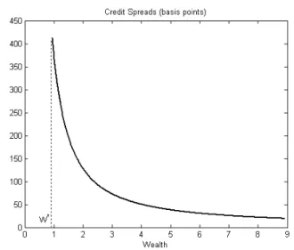
pushes up the corresponding coupon, and hence the default boundary (see (34)), and thus increases the probability of default. Again, we can see that the sanctions effect has stronger impact on credit spread than the value of collateralized fractionβ.OnÞgure 11 we depict the relationship between credit spreads and the volatility of the country’s risky production technology. Clearly, the riskier the technology, the higher is the probability of default, and thus spreads increase. Figure 12 shows that credit spreads increase as the lender’s bargaining power parameter α becomes smaller. Indeed, if the lender knows that he has a weaker position during renegotiations, he will require a higher premium ex-ante. Finally, onÞgure 13 we plot credit spreads against the country’s wealth. We can see that credit spreads increase substantially as the country approaches its default boundary. This fact, together with ourÞnding that the country’s international reserves diminish substantially near the default boundary, conÞrm the empirical Þnding of
Duffie, Pedersen and Singleton (2003) about the inverse relationship between the spreads of Russian GKO and Russian foreign currency reserves.
7
Concluding remarks
In the paper we characterized the behavior of the sovereign borrower who borrows from abroad and in the same time invests at the risk free rate his international reserves. We have derived the conditions under which such kind of behavior is feasible. In the paper we show that the existence of the threat of sanctions is a necessary condition for the contract space to be non-empty. Else, we perform numerical simulations which indicate that the opportunity for the lender to seize collateral does not play a crucial role in contracting. Neither borrower’s gains from the borrowing, nor credit spreads change substantially when the value of collateral changes.
We formulated necessary conditions for the borrower and the lender to sign debt contract at time 0, and also the condition for renegotiations to take place when the borrower defaults. The existence of the risk-free lending opportunities for the borrower allowed us to derive explicit and implicit analytical solutions for the value function as well as optimal consumption and investment strategies for the sovereign country. Also, we obtained the analytical solution for the default boundary. We have shown that near the default boundary the country gears up the consumption rate as well as the risky technology investment fraction at the expense of available international reserves.
To test our model empirically, one would need to estimate all its pa-rameters. Even though this set of parameters is not very big, it might be very difficult to estimate some of them. For example, it may not be easy to estimate the country’s risk aversion parameterγ,to estimate the ex-ante sanctions effect∆µ, the value of the collateralized fraction β,etcetera. We also realize that the model is restricted by a set of assumptions about the val-ues of certain parameters. Relaxing some of those assumptions, for instance assumption 2, may lead to inability to solve the problem analytically.
Our model can be extended to the dynamic case, i.e. when repeated borrowing is allowed, by following Chang and Sundaresan (2000). By doing that one still can expect to obtain all the results in the analytical form. For further research, it would be interesting to introduce asymmetric information in the model, when, for example, the lender cannot perfectly observe the initial wealth of the borrower or cannot monitor the borrower’s wealth during the renegotiation period.
References
Bulow J. and Rogoff K., ”A Constant Recontracting Model of Sovereign Debt”,Journal of Political Economy,97, (1989a), 155-178.
Bulow J. and RogoffK., ”Is forgive to forget?”,American Economic Review, 79, (1989b), 43-50.
Chang G. and Sundaresan S.M., ”A model of dynamic sovereign borrowing: effect of reputation and sanctions”, (2000), Working paper.
Chang G. and Sundaresan S.M., ”Asset prices and default-free term struc-ture in equilibrium model of default”, 1999, Working paper.
Duffie D., Pedersen L. and Singleton K., Modeling Sovereign Yield Spreads: A Case Study of Russian Debt,Journal of Finance, 58, (2003),119-159. Eaton J. and Gersovitz M., ”Debt with potential Repudiation: theoretical and Empirical analysis”, Review of Economic Studies,48, (1981), 288-309. Fleming W.H. and Rishel R.W., ”Deterministic and stochastic optimal con-trol”, Springer-Verlag, 1975.
Gibson R. and Sundaresan S.M., ”A model of sovereign borrowing and sovereign yield spreads”, 2000, Working paper.
Karatzas I.,Lehoczky J.P. Sethi S.P and Shreve S.E., ”Explicit solution of a general consumption/investment problem”, Mathematics of Operations Re-search,2, (1986), 261-294.
Merton, R., ”Optimum consumption and Portfolio Rules in a Continuous Time Model”,J.Econ.Theory,3, (1971), 373-413.
Merton, R., ”On the pricing of corporate debt: the risk structure of interest rates”, Journal of Finance,29, (1974), 449-470.
Merton, R. ”Continuous Time Finance”, Basil Blackwell Inc., Cambridge, 1990.
Westphalen M., Valuation of Sovereign Debt with Strategic Defaulting and Rescheduling, 2001, HEC Lausanne, Dissertation paper.
Figure 1. Relative certainty equivalence as a function of the contractual loan valueI∗for different values of sanctions effect∆µ=µ−ˆµ(µ= 0.1)and collateralized fractionβ. All the other parameters are benchmark ones.
Figure 2. Relative certainty equivalence as a function of the contractual loan valueI∗ for different values of the bargaining power parameterα. All the other parameters are benchmark ones.
Figure 3. Normalized consumption as a function of country’s wealth W for different values of sanctions effect∆µ=µ−µˆ(µ= 0.1).When∆µ= 0.03 :I∗ = 0.3,C¯ = 0.0194;.when ∆µ = 0.02 : I∗ = 0.2,C¯ = 0.012. All the other parameters are benchmark ones.
Figure 4. Normalized consumption as a function of country’s wealthWfor different values of collateralized fractionβ.All the other parameters are benchmark ones.
Figure 5. Risky technology investment fractionωas a function of country’s wealthW for different values of sanctions effect∆µ(µ= 0.1).When∆µ= 0.03 :I∗ = 0.3,C¯ = 0.0194;.when ∆µ = 0.02 : I∗ = 0.2,C¯ = 0.012. All the other parameters are benchmark ones.
Figure 6. Risky technology investment fractionωas a function of country’s wealthW for different values of collateralized fractionβ.All the other parameters are benchmark ones.
Figure 7. The country’s holdings in international reserves (in %) a function of wealthW when∆µ = 0.03, I∗ = 0.3,C¯ = 0.0194and the default boundaryW∗ = 0.9361. All the other parameters are benchmark ones.
Figure 8. The country’s relative risk aversion as a function of wealthWfor different values of sanctions effect∆µ(µ= 0.1).When∆µ= 0.03 :I∗ = 0.3,C¯ = 0.0194;.when ∆µ= 0.02 :I∗ = 0.2,C¯ = 0.012.All the other parameters are benchmark ones.
Figure 9. The country’s relative risk aversion as a function of wealthW for different values of collateralized fractionβ.All the other parameters are benchmark ones.
Figure 10. Credit spread as a function of the contractual loan valueI∗for different values of sanctions effect∆µ (µ= 0.1)and collateralized fractionβ.
Figure 11. Credit spread as a function of the contractual loan valueI∗ for different values of volatility of the risky technologyσ.All the other parameters are benchmark ones.
Figure 12. Credit spread as a function of the contractual loan valueI∗for different values of the bargaining power parameterα.All the other parameters are benchmark ones.
Figure 13. Credit spread as a function of the country’s wealth.Wwhen∆µ= 0.03, I∗ = 0.3,C¯= 0.0194and the default boundaryW∗ = 0.9361All the other parameters are benchmark ones.