Cost-based Modeling for Fraud and Intrusion Detection:
Results from the JAM Project
Salvatore J. Stolfo, Wei Fan
Computer Science Department
Columbia University
500 West 120th Street, New York, NY 10027
f
sal,wfan
g@cs.columbia.edu
Wenke Lee
Computer Science Department
North Carolina State University
Raleigh, NC 27695-7550
Andreas Prodromidis
iPrivacy
599 Lexington Ave., #2300, New York, NY 10022
Philip K. Chan
Computer Science Department
Florida Institute of Technology
150 W. University Blvd., Melbourne, FL 32901
Abstract
In this paper we describe the results achieved using the JAM distributed data mining system for the real world prob-lem of fraud detection in financial information systems. For this domain we provide clear evidence that state-of-the-art commercial fraud detection systems can be substantially improved in stopping losses due to fraud by combining mul-tiple models of fraudulent transaction shared among banks. We demonstrate that the traditional statistical metrics used to train and evaluate the performance of learning systems, (i.e. statistical accuracy or ROC analysis) are misleading and perhaps inappropriate for this application. Cost-based metrics are more relevant in certain domains, and defin-ing such metrics poses significant and interestdefin-ing research questions both in evaluating systems and alternative mod-els, and in formalizing the problems to which one may wish to apply data mining technologies.
This paper also demonstrates how the techniques devel-oped for fraud detection can be generalized and applied to the important area of Intrusion Detection in networked in-formation systems. We report the outcome of recent evalu-ations of our system applied to tcpdump network intrusion data specifically with respect to statistical accuracy. This work involved building additional components of JAM that we have come to call, MADAM ID (Mining Audit Data for
Automated Models for Intrusion Detection). However, tak-ing the next step to define cost-based models for intrusion detection poses interesting new research questions. We scribe our initial ideas about how to evaluate intrusion de-tection systems using cost models learned during our work on fraud detection.
1
Introduction
In this paper we discuss the results achieved over the past several years on the JAM Project1. JAM stands for Java
Agents for Meta-Learning. JAM was initiated as a DARPA and NSF sponsored research project studying algorithms, techniques and systems for distributed data mining. The ini-tial conceptions that we proposed involves the use of agent-based technologies to dispatch machine learning and data analysis programs to remote database sites, resulting in a distributed collection of derived models [4, 5, 6, 25]. Sub-sequently, the same agent-based technology provides the means for derived “base” models to migrate in a network in-formation system and be collected at any of the participating sites where they may be combined. A single “aggregate”
1Browse http://www.cs.columbia.edu/˜sal/JAM/
PROJECTfor the complete set of progress reports, publications and JAM software available for download.
model would then be computed by combining the remotely computed base models, by a technique we have called “meta-learning”, that outputs a “meta-classifier”. Each par-allel site may compute its own meta-classifier, trained on locally stored data. These meta-classifiers likewise can mi-grate around the network to be combined with each other in a hierarchical fashion. The architecture of JAM has been reported extensively in prior papers [24, 26].
JAM’s utility has been demonstrated in the context of real-world problems that in and of themselves are very im-portant. Fraud and intrusion detection are key elements of a new national challenge to protect our nation’s critical in-frastructures.
2
The Fraud Detection Problem
We consider the problem of detecting fraudulent transac-tions after they have been subject to fraud prevention meth-ods and processes. There is a vast literature on various secu-rity methods to protect transactors from unauthorized use or disclosure of their private information and valuable assets.
Financial institutions today typically develop custom fraud detection systems targeted to their own asset bases. The key concept in fraud detection is that fraud may be de-tected by noticing significant deviation from the “normal behavior” of a customer’s account. The behavior of an ac-count can thus be used to protect that acac-count. Notice, it is considerably easier to steal someone’s identity information than it is to steal their behavior2.
Recently though, banks have come to realize that a uni-fied, global approach is required to detect fraud, involving the periodic sharing with each other of information about attacks. We have proposed a new wall of protection consist-ing of pattern-directed inference systems usconsist-ing models of fraudulent transaction behaviors to detect attacks. This ap-proach requires analysis of large and inherently distributed databases of information about transaction behaviors to pro-duce models of “probably fraudulent” transactions. We have used JAM to compute these models.
JAM is used to compute local fraud detection agents that learn how to detect fraud and provide intrusion detection services within a single information system; JAM provides an integrated meta-learning system that combines the col-lective knowledge acquired by individual local agents from among participating bank sites. Once derived local classi-fier agents or models are produced at some datasite(s), two or more such agents may be composed into a new classifier agent by JAM’s meta-learning agents. JAM allows financial institutions to share their models of fraudulent transactions
2This may change as vast databases of “click data” revealing personal
behavior information continues to be acquired over the Internet typically without the user’s knowledge.
by exchanging classifier agents in a secured agent infras-tructure. But they will not need to disclose their proprietary data. In this way their competitive and legal restrictions can be met, but they can still share information. The meta-classifiers then act as sentries forewarning of possibly fraud-ulent transactions and threats by inspecting, classifying and labeling each incoming transaction.
2.1 The Fraud Learning Task
The learning task here is quite straightforward. Given a set of “labeled transactions”,
T
=ft
jt
=< f
1
::: f
n
>
g,
compute a model or classifier,
C
, by some learning algo-rithmL
, that predicts from the features< f
1::: f
n
;1>
the target class label
f
n
, “fraud” or “legitimate”. Hence,C
=L
(T
), whereL
is a learning algorithm. Each elementt
2T
is a vector of features, where we denotef
1 as the
“transaction amount” (tranamt), and
f
n
as the target class label, denotedfraud
(t
)=0 (legitimate transaction) or 1 (afraudulent transaction). Given a “new unseen” transaction,
x
, with unknown class label, we computef
n
(x
) =C
(x
).C
serves as our fraud detector.Much of our work on the JAM project has focussed on developing, implementing and evaluating a range of learn-ing strategies and combinlearn-ing techniques. Our work on “meta-learning” strategies has focussed on computing sets of “base classifiers” over various partitions or samplings of the training data,
T
, and various performance metrics to evaluate base classifiers over test data. (Nearly all of our reported results are based upon k-fold cross validation.)In meta-learning, we first seek to compute a set of base classifiers, f
C
i
i
= 1::: m
g, whereC
i
=L
j
(T
k
), Sk
T
k
=T
, varying the distributions of training data (T
k
)and using a variety of different machine learning algorithms (
L
j
) in order to determine the “best” strategies for building good fraud detectors. The “best” base classifiers are then combined by a variety of techniques in order to boost per-formance. One of the simplest combining algorithms pro-posed in[3], and independently by Wolpert[29], is called “class-combiner” or “stacking”. A separate hold out train-ing dataset,V
, is used to generate a meta-level training data to learn a new “meta-classifier”M
.M
is computed by learning a classifier from training data composed of the predictions of a set of base classifiers generated over a set of validation data (V
) along with the true class label. Hence,M
=L
(< C
1
(
v
)::: C
m
(v
)f
n
(v
)>
)v
2V
.The resultant meta-classifier works by inputing the pre-dictions for some unknown into its constituent base clas-sifiers, and then generating its own final class prediction from these base classifier predictions. Thus, for unknown
x
,f
n
(x
)=M
(C
1
(
x
)::: C
m
(x
)).Notice,
M
is as well a classifier, or fraud detector. In the following sections when we make reference to aclassi-fier
C
, it may either be a “base classifier”, or an ensemble “meta-classifier”, learned over some training distribution, unless explicitly stated otherwise.For notational convenience, we define
J
=F
LMTD
T
] as the set of all classifiers that maybe computed where
L
=fL
1::: L
p
gis a set of learning algorithms,M
fM
1::: M
q
g is a set of meta-learningalgorithms,
T
is a set of labeled ground truth data used to train classifiers, andD
T
is some training distribution of interest. JAM is a computational environment that is designed to assist data miners in generating desired classifiers.2.2 Credit Card Datasets
Chase and First Union Banks, members of the FSTC (Fi-nancial Services Technology Consortium) provided us with real credit card data for our studies. The two data sets con-tain credit card transactions labeled as fraudulent or legiti-mate. Each bank supplied .5 million records spanning one year with 20% fraud and 80% non-fraud distribution for Chase bank and 15% versus 85% for First Union bank. The schemata (or feature sets) of the databases were developed over years of experience and continuous analysis by bank personnel to capture important information for fraud detec-tion. We cannot reveal the details of the schema beyond what is described in [19]. The records have a fixed length of 137 bytes each and about 30 attributes including the bi-nary class label (
f
n
). Some of the fields are numeric and the rest categorical, i.e. numbers were used to represent a few discrete categories.The features in this data defined by the banks essen-tially describe the “usage behavior” of an individual credit card account. The data is rich enough to allow alternative modeling strategies. For example, it is possible to segment the data into classes of accounts based upon “payment his-tory”3. It is well known that there are at least two classes of card holders, “transactors” who pay their bills in full each month, and “revolvers” who pay their minimum charge and roll over balances and interest charges to the next month. Models can thus be built for each of these market segments to determine finer distinctions between account transaction behaviors. In this work, we do no such segmentation and partitioning, but rather we compute models of “fraudulent transaction” for the entire asset base. We believe the results achieved in this study can be improved had we segmented
3The reader is encouraged to do a personal study of their own checking
account behavior. You will likely find the same type of payments from month to month in your own checking account. Variations or distinct pay-ments in any particular month are likely to reoccur in the same month in the prior year. Such repetitive behaviors can be regarded as a normal profile for the checking account. Significant variations from this normal profile possibly indicate fraud.
the data4.
Many experiments were conducted using JAM to eval-uate the performance of different learning algorithms, and different meta-level training sets using this data. Prior pub-lications report on these experiments and indicate that the meta-classifiers consistently outperform the best base clas-sifiers. Unfortunately, the studies that considered different training distributions, different learning algorithms and a variety of combining techniques demonstrated that the best strategies for this target domain are not immediately dis-cernible, but rather requires extensive experimentation to find the best models, and the best meta-classifiers [20].
2.3 Cost-based Models for Fraud Detection
Most of the machine learning literature concentrates on model accuracy (either training error or generalization er-ror on hold out test data computed as overall accuracy, True Positive/False Positive rates, or ROC analysis). This do-main provides a considerably different metric to evaluate performance of learned models; models are evaluated and rated by a “cost model.” Within the context of financial transactions, cost is naturally measured in dollars. How-ever, any unit of measure of utility applies here. The credit card domain provides an excellent motivating example do-main familiar to most people.
Due to the different dollar amounts of each credit card transaction and other factors, the cost of failing to detect a fraud varies with each transaction. Hence, the cost model for this domain is based on the sum and average of loss caused by fraud. We define for a set of transactions
S
, a fixed overhead amount, and a fraud detector (or classifier)C
: CumulativeCost(SC
overhead)=n
Xt
2S
Cost(C
(t
overhead)) and AverageCost(SC
overhead)= CumulativeCost(SC
overhead)n
where Cost(
t
overhead)is the cost associated withtransac-tion
t
andn
is the total number of transactions in a test setS
. The cost of a transaction is not simply its “transaction amount”, but is also a function of an overhead amount.After consulting with a bank representative, we jointly settled on a simplified cost model that closely reflects real-ity. Since it takes time and personnel to investigate a po-tential fraudulent transaction, a fixed overhead value is in-curred for each investigation. That is, if the amount of a
4However, such a strategy would delve dangerously close to industry
Outcome Cost(t,overhead) Miss (False Negative, FN) tranamt(t)
False Alarm (False Positive, FP) overhead if tranamt(t)
>
overhead 0 if tranamt(t)overheadHit (True Positive, TP) overhead if tranamt(t)
>
overhead tranamt(t) if tranamt(t)overheadNormal (True Negative, TN) 0
Table 1. Cost Model for Transaction transaction is smaller than the overhead, it is not worthwhile
to investigate the transaction even if it is suspicious. For ex-ample, if it takes ten dollars to investigate a potential loss of one dollar, it is more economical not to investigate. Assum-ing a fixed overhead, we devised the cost model for each transaction t and classifier C, showed in Table 1. (Recall,
f
1(
t
)=tranamt(t
).) The overhead threshold, for goodrea-son, is a closely guarded secret for important reasons dis-cussed later in section 5.5, and may vary over time. The range of values used in our studies is probably reasonable as appropriate bounds for the data set provided by the banks. All the empirical studies we conducted are evaluated using this cost model.
It is important to note that this overhead is not a “score threshold” for classifiers that may output continuous values (i.e., density estimators). Rather, the threshold is a simple “decision boundary”. Transactions whose amounts are un-der this threshold are immediately authorized (subject to ac-count credit availability of course). Decisions are therefore made by detectors only for transactions above this thresh-old5.
The target application is described as detecting frauds to minimize cumulative cost, or maximize cost savings in this model. In describing our results, we report the maximum savings (or stop loss in bank parlance), as the total dollar amount saved from detection under this cost model. The to-tal potential dollar loss for a (test) set of transactions (
S
) is defined as the total dollar amount of all fraudulent transac-tions:TotalPotentialLoss(S)=
X
t
2S
&fraud(t
)=truetranamt(
t
)A complete comparative evaluation between purely sta-tistical error rates versus cost-model savings can be found in
5When training classifiers, one may think that simply ignoring all
trans-actions in the training data under the threshold will produce better detec-tors. This may not be true. The fraudulent transaction behavior we seek to learn may not vary with the transaction amount (thieves will do the same things whether stealing ten dollars, or a hundred dollars), and the learn-ing of fraudulent behavior may be more accurate when studylearn-ing low cost transactions. Even so, some experiments were performed varying the un-derlying distributions, and we describe these later.
the cited papers. The important lesson here is that the data mining problem is actually a straightforward cost optimiza-tion problem, namely to capture or recover the TotalPoten-tialLoss due to fraud. That is, given a test set of transac-tions,
S
, a fraud modelC
overhead, and the overhead, the TotalCostSavings is defined as:TotalCostSavings(
SC
overhead
overhead)=TotalPotentialLoss(
S
);CumulativeCost(
SC
overhead
overhead)We can now state concretely what the learning task is for fraud detection. We seek to compute the
argmax
C
ov er head2J
f
TotalCostSavings
(SCoverhead
)gwhere individual classifiers,
C
overhead, can be models computed (by JAM) over training data under the cost model with a fixed overhead,T
, by many different learning and meta-learning strategies. (Note, the worst possible outcome is that the detector is so bad we actually lose money; the total cost savings may be negative.) We may of course add additional constraints onC
overhead so that it, for exam-ple, meets real-time, or memory constraints, or is computed over inherently distributed data (partitions ofT
) as rapidly as possible. Explorations of these issues have been much of the focus of the JAM project.It is interesting to note here another reason why pure ac-curacy measures are inappropriate in some domains. Ob-serve in this and related domains (like cellular phone fraud) the distribution of frauds may constitute a very tiny percent-age of the total number of transactions. If, for example, the percentage of frauds is 1% or less, than the null detector will be 99% accurate or better! Naturally, we must depend upon at least the TP/FP rates of a detector to measure alternatives. But, more to the point, training detectors in such domains begs an important question: what is the appropriate distribu-tion of data used in training to produce “good detectors”? In our prior work many experiments were conducted to evalu-ate classifier performance over different samplings and dis-tributions. For example, in one set of tests, 50:50
distribu-tions produced the best detectors6. Of particular note is that the best training distributions varied according to the over-head and thus the cost-model. This is why we subscript the classifier
C
overhead to reveal that alternative classifiers can be computed simply by varying this quantity. Here again, determining the best training distribution under realistic en-vironments, with possibly highly skewed distributions is a matter of considerable empirical investigation.3
Results using JAM
A large number of experiments were performed to deter-mine whether various alternative training strategies would produce improved or superior models. The strategies in-cluded different temporal distributions (different months of training data), different partitions or samples (random, or different distributions of fraud versus non-fraud) and dif-ferent cost distributions (training over large frauds versus lower cost frauds). The results we report here are only one broad view of what we achieved using the best strategies de-termined empirically as compared to the best possible out-come for a commercial off the shelf system.
CHASE provided us with data that had embedded within each transaction record a field recording a score (in the range of 0-999) generated by a commercial off-the-shelf (COTS) fraud detection system for that transaction. From this information we were able to easily compute the best possible detection cost savings of this system as well as its statistical accuracy. We do not know what the actual score thresholds may be in practice. However, for the same data provided by CHASE we can compute what the optimal set-ting for the COTS should be for optimal performance. 7 Using this, we were able to compare JAM’s models to see if we were indeed doing better.
3.1 Baseline Performance Under the Cost Model
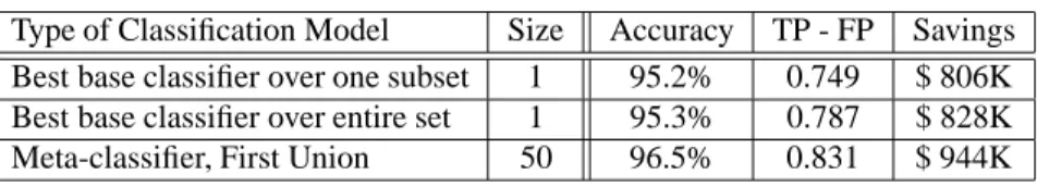
Tables 2 and 3 summarize our results for the Chase and First Union banks respectively. Both tables display the ac-curacy, the TP;FP spread and savings for each of the fraud
predictors examined. Recall, overall accuracy is simply the percentage of correct predictions of a classifier on a test set of “ground truth”. TP means the rate of predicting “true positives” (the ratio of correctly predicted frauds over all of the true frauds), FP means the rate of predicting “false pos-itives” (the ratio of incorrectly predicted frauds over those test examples that were not frauds, otherwise known as the “false alarm rate”.) We use “TP;FP spread” to indicate
6In this context, data is plentiful, so we could afford to construct
many alternative distributions without much fear of generating “knowledge poor” training samples.
7We computed the performance of the COTS for a whole range of score
thresholds: 5, 10, 20, 30, 40, 50, 100, 150, 200, 250, ... , 850, 800, 950.
how well the system finds true frauds versus false alarms. A “1.00 TP;FP spread” is optimal performance.
8
The maximum loss potential of these test sets is approximately $1,470,000 for the Chase data and $1,085.000 for the First Union data. The column denoted as “size” indicates the number of base-classifiers used in the meta-classifier.
3.2 JAM versus COTS
The first row of Table 2 shows the best possible perfor-mance of Chase’s own COTS authorization/detection sys-tem on this data set. The next two rows present the perfor-mance of the best base classifiers over the entire set and over a single month’s data, while the last rows detail the perfor-mance of the unpruned (size of 50) meta-classifiers. Similar data is recorded in Table 3 for the First Union set, with the exception of First Union’s COTS authorization/detection performance (it was not made available to us).
The outcome was clearly in favor of JAM for this dataset. According to these results, the COTS system achieves 85.7% overall accuracy, 0.523 “TP;FP spread” and saves
$682K when set to its optimal “score threshold”.
A comparison of the results of Tables 2 and 3 indicates that in almost all instances, meta-classifiers outperform all base classifiers, and in some cases by a significant margin. The most notable exception is found in the “savings” col-umn of Chase bank where the meta-classifier exhibits re-duced effectiveness compared to that of the best base clas-sifier.
This shortcoming can be attributed to the fact that the learning task is ill-defined. Training classifiers to distin-guish fraudulent transactions is not a direct approach to maximizing savings (or the TP;FP spread). Traditional
learning algorithms are not biased towards the cost model and the actual value (in dollars) of the fraud/legitimate la-bel; instead they are designed to minimize statistical mis-classification error. Hence, the most accurate classifiers are not necessarily the most cost effective. Similarly, the meta-classifiers are trained to maximize the overall accuracy not by examining the savings in dollars but by relying on the predictions of the base-classifiers. Naturally, the meta-classifiers are trained to trust the wrong base-meta-classifiers for the wrong reasons, i.e. they trust the base classifiers that are most accurate instead of the classifiers that accrue highest savings.
3.3 Bridging Classifiers for Knowledge Sharing
The final stage of our experiments on the credit card data involved the exchange of base classifiers between the two
8These are standard terms from the statistical “confusion” matrix that
Type of Classification Model Size Accuracy TP - FP Savings COTS scoring system from Chase - 85.7% 0.523 $ 682K Best base classifier over one subset 1 88.5% 0.551 $ 812K Best base classifier over entire set 1 88.8% 0.568 $ 840K Meta-classifier, Chase 50 89.6% 0.621 $ 818K Table 2. Performance results for the Chase credit card data set. Type of Classification Model Size Accuracy TP - FP Savings Best base classifier over one subset 1 95.2% 0.749 $ 806K Best base classifier over entire set 1 95.3% 0.787 $ 828K Meta-classifier, First Union 50 96.5% 0.831 $ 944K Table 3. Performance results for the First Union credit card data set. banks. To meta-learn over a set of classifier agents,
how-ever, we had to overcome additional obstacles in order to share their knowledge of fraud. The two databases had dif-ferences in their schema definition of the transactions, and hence learning over these different sites produced incom-patible classifiers:
1. Chase and First Union defined an attribute with dif-ferent semantics (i.e. one bank recorded the number of times an event occurs within a specific time period while the second bank recorded the number of times the same event occurs within a different time period). 2. Chase includes two (continuous) attributes not present
in the First Union data.
To address these problems we followed the approaches described in [14, 21, 18]. For the first incompatibility, we had the values of the First Union data set mapped via a lin-ear approximation to the semantics of the Chase data. For the second incompatibility, we deployed special bridging agents that were trained to compute the missing values of First Union data set. The training involved the construc-tion of regression models [23] of the missing attributes over the Chase data set using only the attributes that were com-mon to both banks. When predicting, the First Union clas-sifier agents simply disregarded the real values provided at the Chase data sites, while the Chase classifier agents re-lied on both the common attributes and the predictions of the bridging agents to deliver a prediction at the First Union data sites.
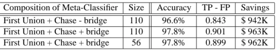
Tables 4 and 5 display the accuracy, TP;FP spread and
cost savings of each Chase and First Union meta-classifier. These results demonstrate that both Chase and First Union fraud detectors can be exchanged and applied to their re-spective data sets. The most apparent outcome of these ex-periments is the superior performance of the First Union meta-classifiers and the lack of improvement on the perfor-mance of the Chase meta-classifiers This phenomenon can
be easily explained from the fact that the attributes missing from the First Union data set were significant in modeling the Chase data set. Hence, the First Union classifiers are not as effective as the Chase classifiers on the Chase data, and the Chase classifiers cannot perform at their best at the First Union sites without the bridging agents. The latter was verified by a separate experiment, similar to the above, with the exception that no bridging agents were used, i.e. Chase classifiers produced predictions without using any informa-tion on the missing values.
The bottom line is that our hypothesis was correct: bet-ter performance resulted from combining multiple fraud models by distributed data mining over different transac-tion record sources (including multiple banks) even when bridging the differences among their schema.
3.4 Cost-sensitive Learning: AdaCost
Much of our experimental work has been to “bias” the outcome of the learned classifiers towards improved cost performance by varying training distributions, or pruning poor cost performing classifiers. This approach is somewhat akin to hammering a square peg into a round hole.
An alternative strategy is called cost sensitive learning. The essence of the idea is to bias feature selection in gen-erating hypotheses during the learning process in favor of those that maximize a cost criterion (for example, the cost of testing features, rather than a purely statistical criterion). According to Turney [28] the earliest work here is due to Nunez [17]. Later work by Tan and Schlimmer [27] also incorporates feature costs in the heuristic for searching in a modified decision tree learning algorithm. However, there are costs associated not only with testing features, but also varying costs based upon classifier misclassification cost performance. The distinctions are important.
Two alternative features may have the same “test cost” but their predictive outcomes may produce different “mis-classification costs.” Hence, we ought to strategically
Composition of Meta-Classifier Size Accuracy TP - FP Savings Chase + First Union 110 89.7% 0.621 $ 800K Chase + First Union 63 89.7% 0.633 $ 877K Table 4. Combining Chase and First Union classifiers on Chase data.
Composition of Meta-Classifier Size Accuracy TP - FP Savings First Union + Chase - bridge 110 96.6% 0.843 $ 942K First Union + Chase + bridge 110 97.8% 0.901 $ 963K First Union + Chase + bridge 56 97.8% 0.899 $ 962K Table 5. Combining Chase and First Union classifiers on First Union data.
choose “low cost features” that are both cheap to compute and test, and that reduce the misclassification cost of the final model that employs them.
What the cost model for the credit card domain teaches is that there are different costs depending upon the outcome of the predictions of the fraud detectors. This may appear strange but we may want to compute classifiers that are purposely wrong in certain cases so that we do not incur their high costs when they predict correctly. Not only are there costs associated with “misclassifications” (False posi-tives/negatives), but also costs are born with Correct Pre-dictions, i.e. True Positives also incur costs (overhead)! This simple, but perhaps counterintuitive, this observation has not been accounted for in prior work and has been in-cluded in our cost models when computing classifiers and evaluating their outcome.
As mentioned, we have performed experiments to gen-erate cost-sensitive classifiers by varying the distribution of training examples according to their costs (tranamt). This strategy doesn’t change the underlying algorithm, but rather attempts to bias the outcome of the underlying (statistical-based) algorithm.
This was achieved by two simple methods: replication and biased sampling. In the first case, experiments were performed where training data was “replicated” some num-ber of times based upon the cost of the exemplars. An-other strategy sampled high cost examples and excluded the low cost transactions (those under the overhead amount). These “cost-based training distributions” were used in train-ing base models, and meta-classifiers. Unfortunately, the results indicated that the resultant classifiers did not consis-tently improve their cost performance [7] over varying cost distributions.
Other experiments were performed to directly bias the internal strategy of the learning algorithm. One algorithm we have proposed and studied is a close variant of Singer and Schapire’s [22] AdaBoost algorithm. AdaBoost is an algorithm that starts with a set of “weak hypotheses” of some training set, and iteratively modifies weights
associ-ated with these hypotheses based upon the statistical per-formance of the hypotheses on the training set. Elements of the training set are as well weighted, and updated on suc-cessive rounds depending upon the statistical performance of the hypotheses over the individual data elements. Ad-aBoost ultimately, therefore, seeks to generate a classifier with minimum training error.
AdaCost [9] is a variant of AdaBoost that modifies its “weight updating rule” by a “cost based factor” (a func-tion of tranamt and the overhead). Here, training elements that are “misclassified” are re-weighted by a function of the statistical performance of the hypotheses as well as the “cost” of the element. Costlier misclassifications are “re-weighted” more for training on the next round. All weights are normalized on each round so correct predictions have their weights reduced. However, the new weights of correct predictions are adjusted by the cost model to account for the cost of true positives as well.
It is not possible to change the underlying training distri-bution according to the credit card cost model because the cost of a transaction is dependent upon the final prediction of the classifier we are attempting to compute, and is not known a priori, i.e., during training. Since the credit card cost model dictates cost even if the classification is correct, adjusting weights of training examples can’t easily reflect that fact. The best we can do here is incorporate the cost for correct predictions on the “current round” during training to produce a different distribution for the “next round” of training.
Experiments here using AdaCost on the credit card data showed consistent improvement in “stopping loss” over what was achieved using the vanilla AdaBoost algorithm. For example, the results plotted in Figure 1 shows the aver-age reduction of 10 months as a percentaver-age cumulative loss (defined as cumulative loss
maximal loss;least loss
100%) for AdaBoost
and AdaCost for all 50 rounds and 4 overheads. We can clearly see that, except for round 1 with overhead = 90, there is a consistent reduction for all other 398(=5024;2)
0.41 0.415 0.42 0.425 0.43 0.435 0.44 0 5 10 15 20 25 30 35 40 45 50
Percentage Cumulative Misclassification Cost
Boosting Rounds OVERHEAD=80 AdaBoost AdaCost 0.43 0.435 0.44 0.445 0.45 0.455 0.46 0.465 0 5 10 15 20 25 30 35 40 45 50
Percentage Cumulative Misclassification Cost
Boosting Rounds
OVERHEAD=90 AdaBoost
AdaCost
Figure 1. Cumulative Loss Ratio of AdaCost and AdaBoost for Chase Credit Card Data Set
We also observe that the speed of reduction by AdaCost is quicker than that of AdaBoost. Figure 2 plots the ratio of cumulative cost by AdaCost and AdaBoost. We have plot-ted the results of all 10 pairs of training and test months over all rounds and overheads. Most of the points are below the “Ratio=1” line in the left drawing and above the “y=x” line in the plot on the right, both implying that AdaCost has lower cumulative loss in an overwhelming number of cases.
4
Intrusion Detection: Initial results using
MADAM ID
Encouraged by our results in fraud detection9, we shifted our attention to the growing problem of intrusion detection in network based systems. Here the problems are signif-icantly different, although from a certain perspective we seek to perform the same sort of task as in the credit card fraud domain. We seek to build models of “normal” behav-ior to distinguish between “bad” (intrusive) connections and “good” (normal) connections.
MADAM ID (Mining Audit Data for Automated Mod-els for Intrusion Detection) is a set of new data mining al-gorithms that were developed by our project specifically to process network intrusion and audit data sets. MADAM ID includes variants of the “association rule” [1, 2] and “fre-quent episodes” [16, 15] algorithms used to define new fea-ture sets that are extracted from labeled tcpdump data in or-der to define training sets for a machine learning algorithm to compute detectors. These features are defined over a set of connections. We first determine what patterns of events in the raw stream appear to occur frequently in attack con-nections that do not appear frequently in normal connec-tions. These patterns of events define “features” computed
9And under “encouragement” from DARPA
for all connections used in training a classifier by some in-ductive inference or machine learning algorithm. The de-tails of this data mining activity have been extensively re-ported [10, 12]. (Our previous exploratory work on learn-ing anomalous Unix process execution traces can be found in [11].) Here we report a summary of our results.
4.1 The DARPA/MIT Lincoln Lab ID Evaluation
We participated in the 1998 DARPA Intrusion Detection Evaluation Program, prepared and managed by MIT Lin-coln Lab. The objective of this program was to survey and evaluate research in intrusion detection. A standard set of extensively gathered audit data, which includes a wide va-riety of intrusions simulated in a military network environ-ment, was provided by DARPA. Each participating site was required to build intrusion detection models or tweak their existing system parameters using the training data, and send the results (i.e., detected intrusions) on the test data back to DARPA for performance evaluation.
We were provided with about 4 gigabytes of compressed raw (binary) tcpdump data of 7 weeks of network traffic, which can be processed into about 5 million connection records, each with about 100 bytes. The two weeks of test data have around 2 million connection records. Four main categories of attacks were simulated: DOS, denial-of-service, e.g., syn flood; R2L, unauthorized access from a re-mote machine, e.g., guessing password; U2R, unauthorized access to local superuser (root) privileges, e.g., various of “buffer overflow” attacks; and PROBING, surveillance and probing, e.g., port-scan.
Using the procedures reported in prior papers [12] we compared the aggregate normal pattern set with the patterns from each dataset that contains an attack type. The fol-lowing features were constructed according to the intrusion
0.8 0.85 0.9 0.95 1 1.05 0 5 10 15 20 25 30 35 40 45 50
Ratio of AdaCost to AdaBoost
Boosting Rounds Ratio=1 Ratio Point 0.3 0.32 0.34 0.36 0.38 0.4 0.42 0.44 0.46 0.48 0.5 0.52 0.3 0.32 0.34 0.36 0.38 0.4 0.42 0.44 0.46 0.48 0.5
AdaBoost Cumulative Cost
AdaCost Cumulative Cost y=x %l of AdaCost and AdaBoost
Figure 2. Cumulative Loss Ratio and Loss of AdaCost and AdaBoost on Chase Credit Card
only patterns:
The “same host” features that examine only the
con-nections in the past 2 seconds that have the same des-tination host as the current connection, and calculate statistics related to protocol behavior, service, etc.
The similar “same service” features that examine only
the connections in the past 2 seconds that have the same service as the current connection.
We call these the (time-based) “traffic” features of the connection records. There are several “slow” PROBING at-tacks that scan the hosts (or ports) using a much larger time interval than 2 seconds, for example, one in every minute. As a result, these attacks did not produce intrusion only pat-terns with a time window of 2 seconds. We sorted these connection records by the destination hosts, and applied the same pattern mining and feature construction process. Rather than using a time window of 2 seconds, we now used a “connection” window of 100 connections, and con-structed a mirror set of “host-based traffic” features as the (time-based) “traffic” features.
We discovered that unlike most of the DOS and PROB-ING attacks, the R2L and U2R attacks don’t have any “in-trusion only” frequent sequential patterns. This is because the DOS and PROBING attacks involve many connections to some host(s) in a very short period of time, the R2L and PROBING attacks are embedded in the data portions of the packets, and normally involves only a single connec-tion. Algorithms for mining the unstructured data portions of packets are still under development. Presently, we use domain knowledge to add features that look for suspicious behavior in the data portion, e.g., number of failed login attempts. We call these features the “content” features.
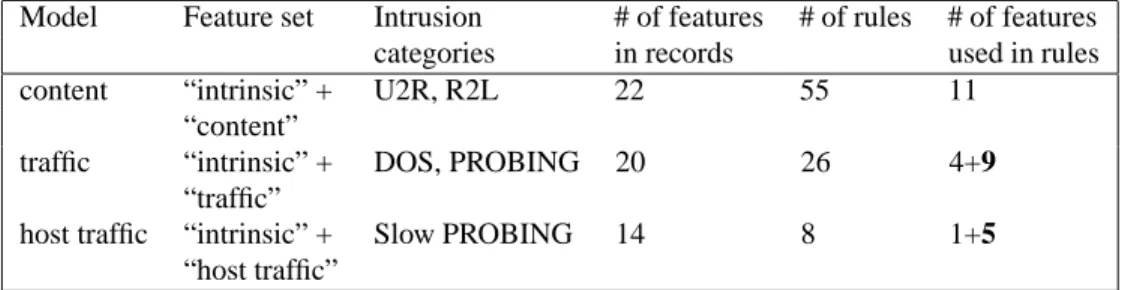
We then built three specialized models, using RIPPER [8]. RIPPER is a rule learning program that outputs a model
quite similar in style to a Prolog program. Each model produced has a different set of features and detects differ-ent categories of intrusions. For example, for the “contdiffer-ent” model, each connection record contains the “intrinsic” fea-tures and the “content” feafea-tures, and the resultant RIPPER rules employing these features detects U2R and R2L at-tacks. A meta-classifier was trained and used to combine the predictions of the three base models when making a fi-nal prediction to a connection record. Table 6 summarizes these models. The numbers in bold, for example, 9, indi-cate the number of automatically constructed temporal and statistical features being used in the RIPPER rules. We see that for both the “traffic” and host-based “traffic” models, our feature construction process contributes the majority of the features actually used in the rules.
4.2 Off-line Detection Results
We report here the performance of our detection models as evaluated by MIT Lincoln Lab. We trained our intrusion detection models, i.e., the base models and the meta-level classifier, using the 7 weeks of labeled data, and used them to make predictions on the 2 weeks of unlabeled test data. The test data contains a total of 38 attack types, with 14 types in the test data only (i.e., our models were not trained with instances of these attack types).
Figure 3 shows the ROC curves of the detection mod-els by attack category as well as on all intrusions. In each of these ROC plots, the x-axis is the false alarm rate, cal-culated as the percentage of normal connections classified as an intrusion; the y-axis is the detection rate, calculated as the percentage of intrusions detected (since the mod-els produced binary outputs, the ROC curves are not con-tinuous). We compare here our models with other par-ticipants (denoted as Group 1 to 3) in the DARPA
eval-Model Feature set Intrusion # of features # of rules # of features categories in records used in rules
content “intrinsic” + U2R, R2L 22 55 11
“content”
traffic “intrinsic” + DOS, PROBING 20 26 4+9 “traffic”
host traffic “intrinsic” + Slow PROBING 14 8 1+5 “host traffic”
Table 6. Model Complexities
uation program (these plots are duplicated from the pre-sentation slides of a report given by Lincoln Lab in a DARPA PI meeting. The slides can be viewed on line via http://www.cs.columbia.edu/˜sal/JAM/ PROJECT/MIT/mit-index.html). These groups pri-marily used knowledge engineering approaches to build their intrusion detection systems. We can see from the fig-ure that our detection models have the best overall perfor-mance, and in all but one attack category, our model is one of the best two.
5
Formalizing Cost-based Models for
Intru-sion Detection
In the credit card fraud domain, the notion of costs is inextricably intertwined with the learning task. We seek to learn models of fraudulent transactions that minimizes the overall loss. We believe an analogous cost optimization problem can and should be defined for the intrusion detec-tion system (IDS) domain.
In the arena of IDS, there are at least three types of costs involved (that are derivative of the credit card fraud case):
1. “Damage” cost: the amount of damage caused by an attack if intrusion detection is not available or an IDS fails to detect an attack;
2. “Challenge” cost: the cost to act upon a potential in-trusion when it is detected; and
3. “Operational” cost: the resources needed to run the IDS.
Table 7 illustrates our perspective on the three types of cost in credit card fraud and intrusion detection. In the credit card case, “damage” is the amount of a fraudulent transaction that the bank losses, tranamt(t). In the IDS case, damage can be characterized as a function that depends on the type of service and attack on that service, DCost(service, attack). The challenge cost for both cases is term as over-head, which is the cost of acting on an alarm. We did not consider operational cost in the credit card case because we did not have the opportunity to study this aspect of the
problem. The banks have existing fielded systems whose total aggregated operational costs have already been con-sidered and are folded into their overhead costs (here called the challenge cost). We shall take a limited view of this by considering the costs of alternative models based upon the “feature costs” used by these models employed in an IDS and we denote this operational cost as OpCost. We next elaborate on each of these sources of cost.
5.1 Damage costs
The damage cost characterizes the amount of damage in-flicted by an attack when intrusion detection is unavailable (the case for most systems). This is important and very dif-ficult to define since it is likely a function of the particu-lars of the site that seeks to protect itself. The defined cost function per attack or attack type should be used here to measure the cost of damage. This means, that rather than simply measuring FN as a rate of missed intrusions, rather we should measure total loss based upon DCost(s,a), which varies with the service (
s
) and the specific type of attack (a
). These costs are used throughout our discussion.5.2 Challenge costs
The challenge cost is the cost to act upon an alarm that indicates a potential intrusion. For IDS, one might con-sider dropping or suspending a suspicious connection and attempting to check, by analyzing the service request, if any system data have been compromised, or system resources have been abused or blocked from other legitimate users. (Other personnel time costs can be folded in including gath-ering evidence for prosecution purposes if the intruder can be traced.) These costs can be estimated, as a first cut, by the amount of CPU and disk resources needed to challenge a suspicious connection. For simplicity, instead of estimat-ing the challenge cost for each intrusive connection, we can “average” (or amortize over a large volume of connections during some standard “business cycle”) the challenge costs to a single (but not static) challenge cost per potential in-trusive connection, i.e., overhead.
0 10 20 30 40 50 60 70 0 0.05 0.1 0.15 0.2 Detection Rate
False Alarm Rate
Columbia Group1 Group2 Group3 (a) DOS 0 10 20 30 40 50 60 70 80 90 100 0 0.05 0.1 0.15 0.2 Detection Rate
False Alarm Rate
Columbia Group1 Group2 Group3 (b) PROBING 0 10 20 30 40 50 60 70 80 0 0.05 0.1 0.15 0.2 Detection Rate
False Alarm Rate
Columbia U2R Group3 U2R Group3 R2L Group1 R2L Columbia R2L (c) U2R and R2L 0 10 20 30 40 50 60 70 0 0.05 0.1 0.15 0.2 Detection Rate
False Alarm Rate
Columbia Group1 Group3
(d) Overall
Figure 3. ROC Curves on Detection Rates and False Alarm Rates
5.3 Operational costs
The cost of fielding a detection system is interesting to consider in some detail. In the work on fraud detection in fi-nancial systems, we learned that there are a myriad of “busi-ness costs” involved in design, engineering, fielding and use (challenge) of detection systems. Each contributes to an overall aggregated cost of detecting fraud. The main issue in operational costs for IDS is the amount of resources to extract and test features from raw traffic data. Some fea-tures are costlier than others to gather, and at times, costlier features are more informative for detecting intrusions. Real-time constraints in IDS. Even if one designs a good detection system that includes a set of good features that well distinguish among different attack types, these fea-tures may be infeasible to compute and maintain in real time. In the credit card case, transactions have a 5 second
response constraint (a desired average waiting time). That’s a lot of time to look up, update and compute and test fea-tures, per transaction. In the IDS case, the desired average response rate should be measured in terms of average con-nection times, or even by TCP packet rates, a much smaller time frame, so connections can be dropped as quickly as possible before they do damage.
In the case of IDS it is not obvious when an intrusion can be detected, and when an alarm should be issued. Ideally, we would like to detect and generate an alarm during an on-going attack connection in order to disable it, rather than af-ter the fact when damage has already been done. However, certain models of intrusive connections may require infor-mation only known at the conclusion of a connection! Thus, properly designing an intrusion detection system requires that considerable thought be given to the time at which a detection can and should take place.
Cost Type Credit Card Fraud Network Intrusion Damage tranamt(t) DCost(service,attack)
Challenge overhead overhead
Operational subsumed in overhead OpCost
Table 7. Cost types in credit card fraud and network intrusion
the constraints are really much different between the two task domains. The problem seems to be much harder in the IDS case since we have to accommodate in our cost mod-els the response rate of the system. It seems evident that a slower IDS should be penalized with a higher cost. (In the credit card case we simply ignored this cost.) This impor-tant source of cost however is a major topic of research for IDS, i.e. the computational costs for rapid detection. Our work in this area is new and ongoing. Details of our initial thoughts here can be found in [13].
5.4 Cost Model for IDS
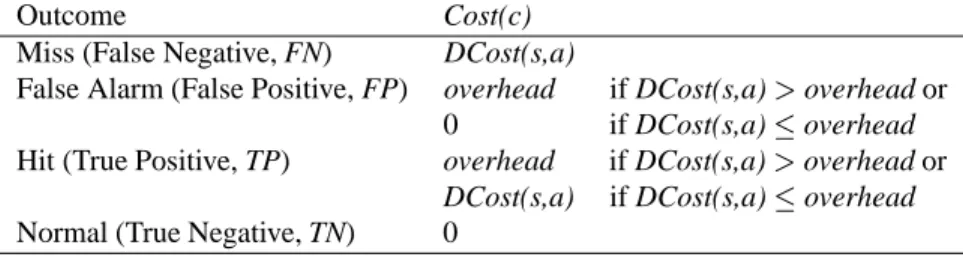
We just described the three different types of cost in IDS: damage cost, challenge cost, and operational cost. Our cost model for IDS considers these three types of cost. Similar to the credit card case, the IDS cost model depends on the outcomes of the IDS’ predictions: false negative (FN), false positive (FP), true positive (TP), and true negative (TN). We now examine the cost associated with each of these out-comes.
FN cost, or the cost of NOT detecting an attack, is the most dangerous case (and is incurred by most systems today that do not field IDS’s). Here, the IDS “Falsely” decides that a connection is not an attack and there is no challenge against the attack. This means the attack will succeed and do its dirty work and presumably some service will be lost, and the organization losses a service of some value. The FN Cost is, therefore, defined as the damage cost associated with the particular type of service and attack, DCost(s,a).
TP Cost is the cost of detecting an attack and doing something about it, i.e. challenging it. Here, one hopes to stop an attack from losing the value of the service. There is a cost of challenging the attack, however, that is involved here. When some event triggers an IDS to correctly predict that a True attack is underway (or has happened), then what shall we do? If the cost to challenge the attack is overhead, but the attack affected a service whose value is less than overhead, then clearly ignoring these attacks saves cost. Therefore, for a true positive, if overhead
>
DCost(sa
),the intrusion is not challenged and the loss is DCost(s,a), but if overhead
<
DCost(sa
), the intrusion is challengedand the loss is limited to overhead.
FP cost. When an IDS falsely accuses an event of be-ing an attack, and the attack type is regarded as high cost, a challenge will ensue. We pay the cost of the challenge
(overhead), but nothing really happened bad except we lost overhead on the challenge. Naturally, when evaluating an IDS we have to concern ourselves with measuring this loss. For this discussion, we define the loss is just overhead for a false positive.
TN cost. An IDS correctly decides that a connection is normal and Truly not an attack. We therefore bare no cost that is dependent on the outcome of an IDS.
Thus far we have only considered costs that depend on the outcome of an IDS, we now incorporate the operational cost, OpCost, that is independent of the IDS’ predictive per-formance. Our notion of OpCost mainly measures the cost of computing values of features in the IDS. We denote Op-Cost(c) as the operational cost for a connection,
c
.We now can describe the cost-model for IDS. When eval-uating an IDS over some test set
S
of labeled connections,c
2S
, we define the cumulative cost for a detector asfol-lows:
CumulativeCost
(S
)= Xc
2S
(Cost
(c
)+OpCost
(c
)) (1) where Cost(c
)is defined (analogous to the credit card case)in Table 8. Here
s
is the service requested by connectionc
anda
is the attack type detected by the IDS for the connec-tion.Note that a higher operational cost, OpCost(c), could be incurred by employing “expensive” features; but this may potentially improve the predictive performance of the IDS and thus lower Cost(c). Hence, in order to minimize Cumu-lativeCost(S), we need to investigate and quantify, in real-istic contexts, the trade off between OpCost(c) and Cost(c) in Equation 1. This issue constitutes a major part of our ongoing research in the JAM project.
5.5 Flying Under Mobile Radar: Dynamic Over-head Adjustment
As in the credit card case, we can simplify the IDS cost model by subsuming the operational costs into overhead (challenge cost). In this way the cumulative cost of an IDS is highly dependent upon the overhead10value set at
10and we may regard the overhead as the minimum height that a radar
Outcome Cost(c) Miss (False Negative, FN) DCost(s,a)
False Alarm (False Positive, FP) overhead if DCost(s,a)
>
overhead or 0 if DCost(s,a)overheadHit (True Positive, TP) overhead if DCost(s,a)
>
overhead or DCost(s,a) if DCost(s,a)overheadNormal (True Negative, TN) 0
Table 8. Cost Model for Connection the time models are computed, and certainly when they are
evaluated. It is quite possible, and virtually assured, that un-der different overheads, different models will be computed and different cost performance will be exhibited.
In some industries (not only the credit card industry), overheads are so firmly fixed that fraud is simply mod-eled as another “cost of doing business” and is simply tol-erated11. The overhead amount is defined by a myriad of
business costs, but it need not be static when applied at run-time! Thus, it is quite logical to vary the overhead limit when operating an IDS, thus changing the challenge cost producing different behavior and cost performance of the detection system. This simple strategy tends to enter “noise” making it difficult for perpetrators to “optimize” their thefts.
But notice that under a changing overhead, either up or down, for which detectors had originally been trained, the outcome of cost savings attributed to the detector might vary widely. This change in overhead has another fundamental effect: it changes the environment from which our underly-ing distribution is drawn. This means, that once we lower the overhead, thieves might learn to lower their appetite for stealing not to get caught. Concurrently, raising the over-head afterwards might then generate large cost savings, un-til the thieves have learned to return to their former ways of being greedy.
An interesting question, therefore, is whether there is an optimal strategy of dynamically varying the overhead in order to maximize savings over a longer period of time. Varying the overhead implies that we must concern our-selves with potentially “non-linear effects” in cost savings. A slight reduction may indeed catch more fraud, but may re-sult in far heavier losses due to the real costs of challenging a new found wealth of “cheap fraud”!
exceptionally interesting task of assuring their flying missiles stay below this radar to deliver their ordinance!
11For example, in the auto insurance industry, broken windshields are
regarded as an immediately approved expense. Fraud perpetrators will sub-mit insurance charges for bogus repairs of windshields and be assured of payment, simply because the cost of investigation is prohibitively expen-sive. Here thieves have a different problem. They need to learn the rate at which they submit bogus claims not to draw obvious attention to them-selves from human claims processing personnel, the low bandwidth, final detectors.
This begs further questions and deeper study to deter-mine alternative strategies. Perhaps classifiers ought to be entirely retrained, or meta-classifiers might re-weight their constituent base classifiers under a new changing fraud and cost distribution, and when should we do this? Or, sim-ply measuring daily cost savings performance, or the rate of change thereof, might provide interesting clues to an opti-mal daily setting? The rate at which we change our over-head setting, and/or our models to avoid widely varying os-cillations in performance of overall cost savings is not ob-vious.
It is interesting to note here that one of the design goals of JAM is to provide a scalable, efficient and hence adapt-able distributed learning system that provides the means of rapidly learning new classifiers, and distributing (via agent architectures) new detectors to accommodate chang-ing conditions of the environment in which it operates. An-other avenue for exploration in JAM is therefore to perhaps dynamically re-weight ensembles of classifiers, our meta-classifiers, to adjust to new overhead limits.
5.6 Summary
In our work on intrusion detection, the data mining ac-tivity was focussed on uncovering likely features to extract from the streaming TCP packets preprocessed into connec-tion records that are used in preparing training data, com-puting models and testing those models.
However, much of the traditional research in modeling only considers statistical accuracy, or TP
=
FP rates of mod-els when comparing approaches. We should now under-stand that accuracy is not the whole picture. In different real world contexts, “cost” can take on different meanings, and the target application might necessarily be defined as a cost optimization problem.In the context of IDS, real time performance is crucial. Here cost measures involve throughput and memory re-sources. It is of no value if one has an IDS that consumes so much resource that services can no longer be delivered on time, or the cost of fielding the IDS is so high that it becomes uneconomical to do so.
6
Conclusion
In this paper, we presented the main results of the JAM project. We focused the discussion on cost-sensitive model-ing techniques for credit card fraud detection and network intrusion detection. We showed that the models built using our distributed and cost-sensitive learning techniques can yield substantial cost savings for the financial institutions. We reported our research in applying data mining tech-niques to build intrusion detection models. The results from the 1998 DARPA Intrusion Detection Evaluation showed that our techniques are very effective. We briefly examined the cost factors and cost models in intrusion detection, and discussed the challenges in cost-sensitive modeling for in-trusion detection.
6.1 Future Work
There a number of open research issues that need to be addressed in the general setting of distributed data mining, but also specific to the important task of detecting intru-sions:
1. How does an organization or domain rationally set the costs of its various services and systems it wishes to protect with an IDS, thus defining Cost(s,a) for all ser-vices and all attack types? And how do we rationally determine an overhead challenge cost, overhead espe-cially under tough real-time constraints?
2. What “cost sensitive” data mining and machine learn-ing algorithms are needed to generate “low cost” mod-els; i.e. models that are cheap to evaluate and operate under (variable) “real-time” constraints, and that also maximize cost savings or minimize loss?
3. Specifically for network-based intrusion detection, what is the optimal set of features to best model a “good detector” for different environments and plat-forms?
4. The distribution of attacks, and the various costs asso-ciated with services and attacks will naturally change over time. What adaptive strategies might be needed to optimally change models or mixtures of models to improve detection and at what rate of change? 5. Likewise, what strategies may be employed in
dynam-ically adjust overhead challenge costs (overhead) to maximize cost savings for a fixed detection system over larger time periods.
In conclusion, we need a microeconomic theory of intru-sion detection.
7
Acknowledgments
This research is supported in part by grants from DARPA (F30602-96-1-0311) and NSF (IRI-96-32225 and CDA-96-25374).
Our work has benefited from in-depth discussions with Alexander Tuzhilin of New York University and Foster Provost of Bell Atlantic research, and suggestions from Charles Elkan of UC San Diego.
References
[1] R. Agrawal, T. Imielinski, and A. Swami. Min-ing association rules between sets of items in large databases. In Proceedings of the ACM SIGMOD Conference on Management of Data, pages 207–216, 1993.
[2] R. Agrawal and R. Srikant. Fast algorithms for mining association rules. In Proceedings of the 20th VLDB Conference, Santiago, Chile, 1994.
[3] P. Chan and S. Stolfo. Meta-learning for multistrat-egy and parallel learning. In Proc. Second Intl. Work. Multistrategy Learning, pages 150–165, 1993. [4] P. Chan and S. Stolfo. Toward scalable and parallel
learning: A case study in splice junction prediction. Technical Report CUCS-032-94, Department of Com-puter Science, Columbia University, New York, NY, 1994. (Presented at the ML94 Workshop on Machine Learning and Molecular Biology).
[5] P. Chan and S. Stolfo. Scaling learning by meta-learning over disjoint and partially replicated data. In Proc. Ninth Florida AI Research Symposium, pages 151–155, 1996.
[6] P. Chan and S. Stolfo. Sharing learned models among remote database partitions by local meta-learning. In Proc. Second Intl. Conf. Knowledge Discovery and Data Mining, pages 2–7, 1996.
[7] P. Chan and S. Stolfo. Learning with non-uniform distributions: Effects and a multi-classifier approach. Submitted to Machine Learning Journal, 1999. [8] W. W. Cohen. Fast effective rule induction. In
Ma-chine Learning: the 12th International Conference, Lake Taho, CA, 1995. Morgan Kaufmann.
[9] W. Fan, S. Stolfo, and J. Zhang. Adacost: Misclassi-fication cost-sensitive boosting. In Proceedings Inter-nation Conference on Machine Learning, 1999.
[10] W. Lee and S. J. Stolfo. Data mining approaches for intrusion detection. In Proceedings of the 7th USENIX Security Symposium, San Antonio, TX, January 1998. [11] W. Lee, S. J. Stolfo, and P. K. Chan. Learning patterns from unix process execution traces for intrusion de-tection. In AAAI Workshop: AI Approaches to Fraud Detection and Risk Management, pages 50–56. AAAI Press, July 1997.
[12] W. Lee, S. J. Stolfo, and K. W. Mok. A data mining framework for building intrusion detection models. In Proceedings of the 1999 IEEE Symposium on Security and Privacy, May 1999.
[13] W. Lee, S. J. Stolfo, and K. W. Mok. Mining in a data-flow environment: Experience in network intru-sion detection. In Proceedings of the ACM SIGKDD International Conference on Knowledge Discovery & Data Mining (KDD-99), August 1999.
[14] Jacek Maitan, Zbigniew W. Ras, and Maria Ze-mankova. Query handling and learning in a dis-tributed intelligent system. In Zbigniew W. Ras, ed-itor, Methodologies for Intelligent Systems, 4, pages 118–127, Charlotte, North Carolina, October 1989. North Holland.
[15] H. Mannila and H. Toivonen. Discovering general-ized episodes using minimal occurrences. In Proceed-ings of the 2nd International Conference on Knowl-edge Discovery in Databases and Data Mining, Port-land, Oregon, August 1996.
[16] H. Mannila, H. Toivonen, and A. I. Verkamo. Dis-covering frequent episodes in sequences. In Proceed-ings of the 1st International Conference on Knowledge Discovery in Databases and Data Mining, Montreal, Canada, August 1995.
[17] M. Nunez. Economic induction: A case study. In Pro-ceedings of the Third European Working Session on Learning, EWSL-88, pages 139–145. Morgan Kauf-mann, 1988.
[18] A. L. Prodromidis and S. J. Stolfo. Mining databases with different schemas: Integrating incompatible clas-sifiers. In G. Piatetsky-Shapiro R Agrawal, P. Stolorz, editor, Proc. 4th Intl. Conf. Knowledge Discovery and Data Mining, pages 314–318. AAAI Press, 1998. [19] A. L. Prodromidis and S. J. Stolfo. Agent-based
dis-tributed learning applied to fraud detection. In Six-teenth National Conference on Artificial Intelligence, 1999. Submitted for publication.
[20] A.L. Prodromidis and S.J. Stolfo. A comparative eval-uation of meta-learning strategies over large and dis-tributed data sets. In Workshop on Meta-learning, Six-teenth Intl. Conf. Machine Learning, 1999. Submitted for publication.
[21] Zbigniew W. Ras. Answering non-standard queries in distributed knowledge-based systems. In L. Polkowski A. Skowron, editor, Rough sets in Knowledge Dis-covery, Studies in Fuzziness and Soft Computing, vol-ume 2, pages 98–108. Physica Verlag, 1998.
[22] R. Schapire and Y. Singer. Improved boosting algo-rithms using confidence-rated predictions. In Proceed-ings of the Eleventh Annual Conf on Computational Learning Theory, 1998.
[23] StatSci Division, MathSoft, Seattle. Splus, Version 3.4, 1996.
[24] S. Stolfo, W. Fan, W. Lee, A. Prodromidis, and P. Chan. Credit card fraud detection using meta-learning: Issues and initial results. Working notes of AAAI Workshop on AI Approaches to Fraud Detec-tion and Risk Management, 1997.
[25] S. Stolfo, W.D. Fan, A. Prodromidis W.Lee, S. Tselepis, and P. K. Chan. Agent-based fraud and intrusion detection in finan-cial information systems. Available from http://www.cs.columbia.edu/ sal/JAM/PROJECT, 1998.
[26] S. Stolfo, A. Prodromidis, S. Tselepis, W. Lee, W. Fan, and P. Chan. JAM: Java agents for meta-learning over distributed databases. In Proc. 3rd Intl. Conf. Knowl-edge Discovery and Data Mining, pages 74–81, 1997. [27] M. Tan and J. Schlimmer. Two case studies in cost-sensitive concept acquition. In Proceedings of the Eight National Conference on Artificial Intelligence, pages 854–860, Boston, MA, 1990.
[28] P. D. Turney. Cost-sensitive classification: Empirical evaluation of a hydrid genetic decision tree induction algorithm. Journal of AI Research, 2:369–409, 1995. [29] D. Wolpert. Stacked generalization. Neural Networks,