Cost efficiency of banks in Croatia
Ivan Huljak
Croatian National Bank, Zagreb, Croatia, ivan.huljak@hnb.hr
Abstract
Foreign and larger banks in Croatia are generally considered to be more cost efficient compared with domestic and smaller banks. However, those views are often based on data from financial statements that can be misleading due to simultaneous consolidation process on the market and the existence of economies of scale. To contribute to the Croatian banking efficiency literature, we construct a panel of individual bank data for 1994-2014 period and conduct a frontier analysis to calculate bank specific X-efficiency. Our results suggest that efficiency scores depend on the cost definition as domestic and smaller banks are more efficient in managing administrative costs compared with foreign and larger banks but equally efficient in managing total costs. Results indicate that average bank relative efficiency increased on two occasions: one in the late 90s in the period of banking crisis and subsequent "market cleansing" and to a lesser extent in the period marked with financial crisis. Although the differences between bank cost efficiencies seem small, we conclude that the area is worth further research as significant gains in bank earnings could be achieved by increasing efficiency.
Keywords: Croatia, banks, cost efficiency. JEL classification: D22, G21, G34.
DOI: 10.1515/crebss-2016-0002 Received: October 15, 2015 Accepted: December 2, 2015
Disclaimer: Any opinions expressed in this research are those of the author and not necessarily those of Croatian National Bank.
Introduction
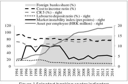
Data from financial statements suggests that the efficiency of banking sector in Croatia increased in the last 20 years. Indeed, banks were able to collect significantly more deposits per unit of labour used and in the same time increase asset per employee. Together this decreased cost to income ratio, which is often used for bank efficiency approximation (Figure 1). It is also often believed that the entrance of foreign owners led to bank efficiency increase as know-how in cost management started to transfer from foreign owners to newly acquired banks. The data shows that standard aggregate efficiency indicators all record constant improvements after the entrance of foreign investors. However, the entrance of foreign players on the market increased market concentration, which stimulated standard efficiency indicators due to economies of scale. Therefore, efficiency gains observed through indicators from financial statements could to a large extent be influenced by economies of scale while actual cost efficiency could be
independent on bank ownership structure or bank size (Figure 1). Therefore, it could be the case that the efficiency of banks did not improve over time, and that the financial crisis did not cause banks to be more efficient, it simply speeded up the process of consolidation on the market. In addition, the data from financial statements does not allow for conclusions about real (empirical) bank efficiency as it cannot control for bank size or the prices bank has to pay on the market. Considering that empirical indicators are rather data consuming and technically challenging to calculate researchers often use various approaches with rather inconsistent results. Therefore, a significant part of economic practice approaches the question of bank efficiency with caution and the question of bank efficiency is often sidelined in research, especially in CEE countries where data quality was until recently one of the constraints for researching this area.
In the Croatian banking context, researchers have examined issues of bank efficiency often in context of specific historic periods marked with privatisation, ownership transfer or regulatory changes. Kraft and Tirtoroglu (1998) used Stochastic Frontier Approach on 1994 and 1995 data to estimate efficiencies for old vs. new and state vs. private banks. They concluded that new banks seem to be more X-inefficient and more scale-X-inefficient than either old privatized banks or old state banks. However, authors emphasize that the relationship between profitability and efficiency between banks in Croatia is statistically weak. Jemrić and Vujčić (2002) used Data Envelopment analysis to conclude that (between 1995 and 2000) foreign-owned banks are on average more efficient compared with domestic banks and that new banks are more efficient than old ones. Authors also find strong equalization in terms of average efficiency in the Croatian banking market, both between peer groups and within peer groups of banks. Kraft, Payne and Hofler (2006) used a flexible Fourier cost function to show that new and privatized banks are not necessarily the most efficient in the period from 1994-2000. In addition, according to their results, privatisation does not seem to be influencing cost efficiency of banks. However, higher cost efficiency is connected with lower bank default probability. Finally, Arisis (2010) in cross-country study and Huljak (2015) in country level study calculated cost efficiency of banks in Croatia to find evidence of Quiet-life hypothesis: market power having a negative, although economically weak, influence on bank efficiency.
The motive of this research is to calculate empirical efficiency of banks in Croatia, but also to provide more explanation on the methodology and perhaps clear some of the reasons why research done so far resulted in inconsistent results. In addition, the data set is relatively long, and enables putting the efficiency results in economic and historical context and observe bank efficiency over the business cycle. Therefore, we contribute to the literature on bank efficiency in Croatia by calculating an empirical measure of bank efficiency for the period 1994-2014, which gives us the opportunity to compare the results with some earlier work on this matter but also test some of the “common knowledge” on this subject.
This paper is organized as follows: After introduction, literature overview and traditional aggregate indicators of bank efficiency in Croatia in Section 1, Section 2 explains the data and the methodology. Section 3 displays and elaborates the results, while Section 4 concludes.
Data and methodology
The groundwork for firm-level efficiency measurement was laid by Farrell (1957), who provided useful information on how to define firm efficiency as a concept, and how to calculate efficiency measures. However, the concept of X-efficiency was
developed later on by Leibenstein (1966) while questioning the assumptions in postulating non-allocative type of efficiency within firm. Eventually, he showed that firms were neither always internally efficient nor always maximizing their profits because of inherent inefficiency that is not of allocative nature and which was called X-efficiency (XE).
Over the years, two main approaches were developed for firm efficiency calculation: parametric and non-parametric with the difference being that parametric methods assume functional form of the frontier up front, while non-parametric methods use linear programming techniques and assume that random error equals zero, neglecting the importance of specification of the individually best practice frontier. Since only parametric models allow for hypothesis testing, more recent literature is more inclined to parametric models. To minimize the problem of confusing inefficiencies from random error, parametric models usually estimate a transcendental log function that allows returns to scale to change with input or output proportions so that the estimated cost curve can have a familiar U-shape. However, within the parametric approach the assumption on the distribution of random errors has to be made for which purpose researchers usually chose between Stochastic Frontier Approach (SFA) and Distribution Free Approach (DFA). SFA determines the functional form for the cost, inputs and prices up front and by using this approach; researchers accept that inefficiencies are half-normally distributed, while errors have a normal distribution. DFA on the other hand separates the inefficiencies from random errors in a different way, as it makes no strong assumption about regarding their distribution.
The application of the frontier methods on banking sector was to a large extent pioneered by Berger (1993) who calculated the XE for United States banks by utilizing a Distribution free approach (DFA) under the assumption that banks efficiencies are relatively stable over time. In addition, Berger, Hunter and Timme (1993) indicated that X-inefficiencies in bank industry account for more than 20 percent of all banking costs, while scale and scope efficiencies together make up to 5 percent. We follow Berger and Hannan (1998) who used DFA to calculate bank XE by measuring the closeness of the bank costs to the minimum costs for the bank’s output that could be achieved on the market. To estimate efficiency authors assume that the cost function has a composite error term that includes both inefficiencies (deviations from the efficient frontier) and random error. The difficulty in estimating efficiency in practice is in drawing the line between the two. The key assumption of DFA is that cost differences owing to inefficiency are relatively stable and should persist over time, while those owing to random error will average out over time and become zero. The bank that could achieve that minimum represents efficiency frontier and all the other banks are compared to that bank. We apply the DFA method to panel data and estimate a regression of trans-log cost function to create statistical connections between costs and observed levels of bank data variables (bank products and input prices). The residuals of these cross-section regressions are assumed to contain random measurement error, temporary variations in costs, and persistent but unknown cost differences attributed to inefficiency. Averaging each banks' residual across a long enough period of time across separate cross-section regressions reduces normally distributed error from trans-log function to minimal levels leaving only average inefficiency. We follow De Young (1997) who calculated that six years of separate cross-section regressions is needed for random error to approach zero. This is the reason why we excluded banks for which the regression does not result with at least six years of residuals.
One has to be aware of the limits of the DFA approach as the measure derived from this method is of a relative nature and therefore is scaled to the most efficient bank. Consequently, no easy-to-use-aggregate number can be achieved and used for commenting the absolute efficiency of banks, as it was not known what was happening with the most efficient bank. Other limit arises from the fact that DFA has to be applied on periods and therefore conclusions cannot be drawn separately for years. Finally, it should be noted that data-truncating procedure is important for any frontier analysis results. The more data is trimmed or winsorized, the higher the efficiency scores will result as differences between average bank and most efficient bank reduce.
For the XE calculation, we use standard trans-log cost function with three inputs (financial capital, labour and physical capital) and three outputs (investments, loans and fees revenue):
M m it it m M m it n mn M m it m N n it n mn M m it m N n it n mn N n it m n M m it m m i itY
W
ab
W
W
b
Y
Y
a
W
b
Y
a
C
, , , , , , , ,ln
ln
ln
ln
2
1
ln
ln
2
1
ln
ln
ln
, (1)where subscripts n is the nth input and m denotes the mth output, i is ith bank, C is cost,
Y is bank product and W is input price.
For the DFA method, a vector cost function is modified, as the error term is decomposed: it i it it it W Y u v C ln( , ) ln ln ln , (2)
where
ln
u
i is inefficiency andln
v
itis measurement error.To calculate efficiency, we average the residuals from equation (2) for each bank over the six years. This average residual, is an estimate of ln(xi) , given that the
random errors ln(vit) will tend to cancel each other out for each firm separately in the
averaging. We transform ln(
u
ˆ
i) into a normalized measure of efficiency:)
ˆ
ln
ˆ
exp(ln
min i iu
u
XE
, (3)where
u
ˆ
iis the average residual from trans-log function for each bank and minindicates the minimum for all i.
This is an estimate of the ratio of costs for the most efficient bank in the sample to bank i costs for bank i combination of outputs and input prices. This corresponds with the conventional notion of efficiency as the ratio of the minimum resources needed for production to the resources actually used, and ranges over (0, 1], with higher values indicating greater efficiency.
On the issue of cost definition, there is no consensus in the literature as authors use different definitions ranging from only administrative costs to total costs including interest costs and sometimes even loan loss provisions. However, it should be noted that using a different cost definition would require a different interpretation and therefore the results of different researches cannot be easily compared. Having this in mind, we calculate our XE using two definitions of costs: narrow (administrative costs) and broad (total costs). However, we do not include loan loss provisions in total costs, as we believe that these costs are the result of credit risk management
and not cost management. In addition, besides, loan loss provisions from today result from decisions made in the past.
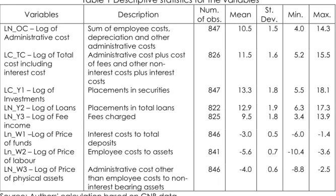
Table 1 Descriptive statistics for the variables
Variables Description of obs. Num. Mean Dev. St. Min. Max. LN_OC – Log of
Administrative cost
Sum of employee costs, depreciation and other administrative costs
847 10.5 1.5 4.0 14.3 LC_TC – Log of Total
cost including interest cost
Administrative cost plus cost of fees and other non-interest costs plus non-interest costs
826 11.5 1.6 5.2 15.5
LC_Y1 – Log of
Investments Placements in securities 847 13.3 1.8 5.5 18.1 LN_Y2 – Log of Loans Placements in total loans 822 12.9 1.9 6.3 17.3 LN_Y3 – Log of Fee
income
Fees charged 825 9.5 1.8 3.4 13.9 Ln_W1 –Log of Price
of funds
Interest costs to total deposits
846 -3.0 0.5 -6.0 -1.4 Ln_W2 – Log of Price
of labour Employee costs to assets 841 -5.6 0.7 -10.4 -3.6 LN_W3 – Log of Price
of physical assets Administrative cost other than employee costs to non-interest bearing assets
846 -4.0 0.6 -8.8 -2.5 Source: Authors' calculation based on CNB data.
The initial sample includes unbalanced panel with 72 banks over 21 years (1994 - 2014) making 876 observations overall. Out of 72, 27 banks were present on the market at the end of 2014 out of which 23 banks were present in the whole sample. The data is collected from statistical and supervisory reports gathered by the Croatian National Bank. The data set is skewed as the number of banks in the sample decreases over time, with the biggest reduction recorded at the beginning of the sample in late nineties when the banking crisis occurred. After 2002, the decrease in the number of banks is continuous but steady and was mostly the result of merger activities. Therefore, after 2002, the structure of the banking system remained relatively stable with concentration levels similar to today’s levels and with foreign institutions owning around 90% of the banking sector assets. In order to compare the results within the banking sector as well as to compare the results with earlier research on this topic, the following groups of banks could be recognized: small banks (banks with market share lower than 1%), big banks (banks with market share higher or equal to 1%), domestic banks (banks whose more than 50% of shares is owned by non-government residents), foreign banks (banks whose more than 50% of shares is owned by non-residents), and government owned banks (banks whose more than 50% of shares is owned by domestic government or agencies). In the whole sample, the majority of bank-year observations refer to smaller banks (569 compared with 278 for bigger bangs). In addition, majority of bank-year observations refer to domestic owned banks (486 compared to 256 for foreign-owned banks and 96 for government foreign-owned banks).
In addition, to remove the outliers from the sample all banks with the implicit interest cost of 50% or more were removed from the sample. Further on, banks with negative costs of physical assets or with depreciation higher than 40% of physical assets were removed, as well. As a result, 28 bank-year observations were removed
and our sample after data trimming consists of 848 bank-year observations Table 1). Because of DFA method nature, which requires at least six-year periods we average only the residuals for banks that were present on the market for at least six years. This leads to further reduction of the number of observations and we therefore derive 476 XE results from 814 residuals. Regarding the model specification, researchers usually use panel OLS for calculating efficiency scores via DFA. We use panel OLS and panel regression with fixed effects for each bank to ensure the robustness of results. We apply Hausman test (1978) for discriminating between random and fixed effects.
Results
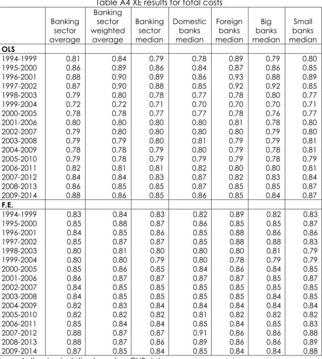
As explained earlier, standard efficiency indicators from financial statements suggest that bank cost efficiency in Croatia increased in the1994-2014 sample (Figure 1). In addition, standard efficiency indicators would suggest that larger institutions are more efficient. However, empirical efficiency indicators show different dynamics and different bank ranking. Our results confirm that bank efficiency scores depend largely on the definition of efficiency used. Our mean XE amounts to 0.75-0.79 for administrative costs and 0.81-0.84 for total costs depending on the model specification (Table 2). Therefore, on average, most efficient bank on the market could offer the same service with the same input prices as average bank by using 75-79 percent of its administrative costs and 81-84 percent of its total costs. Our results also suggest that the XE differences between banks in Croatia are relatively stable over time (Figure 2 and Appendix Table A2).
Figure 1 Selected banking sector indicators Source: Authors' calculation based on CNB data.
Note: Market instability index is calculated according to Hymer and Pashigan (1962). It is the sum of all changes of market shares in a year.
Compared with other research results using frontier analysis, our XE results are similar with results from Kraft and Tirtiroglu (1998) and Ariss (2010). Kraft and Tirtioglu (1998) calculated an average XE for banks in Croatia of around 0.75-0.80 for 1994 and 1995. Our results for total cost efficiency for the 1994-1999 period are 0.81-0.84. Ariss (2010) calculated efficiency for Croatia of 0.83 for 1999-2005 periods, which is close to our result of 0.85. The differences between our results and comparable research result are due to different approach in data trimming and different time horizon used. 0 5 10 15 20 0 20 40 60 80 100 120 1994 1995 1996 1997 1998 1999 2000 2001 2002 2003 2004 2005 2006 2007 2008 2009 2010 2011 2012 2013 2014 Foreign ba nks sha re (%) Cost to income ra tio (%) CR 5 (%) - right
La bour to deposit ra tio (%) - right
Ma rket insta bility index (per.points) - right Asset per employee (HRK million) - right
Table 2 XE descriptive statistics
Variable Obs. Mean Std. Dev. Min Max Administrative costs – OLS 476 0.79 0.08 0.48 1 Administrative costs – F.E. 476 0.75 0.10 0.43 1 Total costs - OLS 472 0.81 0.09 0.52 1 Total costs - F.E. 472 0.84 0.09 0.45 1 Source: Authors' calculation based on CNB data.
Note: OLS stands for Ordinary least squares and F.E. stands for fixed effects.
The fact that the differences are larger in administrative than total cost efficiency could be due to a couple of factors. First, the differences between banks in Croatia regarding business strategy are substantial; some banks are more focused on corporate, some on natural persons and some are universal in full meaning of the word. Therefore, the distribution network that initiates the majority of administrative costs is quite different between banking groups. Also, since administrative costs are relatively small (some 2.5 percent of total assets), it is possible some banks believe that they can afford to be more “comfortable” in managing them.
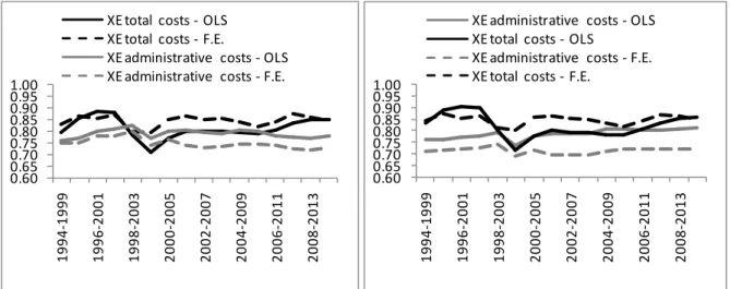
Figure 2 Medial (left) and weighted average (right) bank efficiency Source: Authors' calculation based on CNB data.
Even though one should keep in mind that XE is a relative indicator and that by using the DFA it can be only calculated for periods and not years, it is still possible to show a time dimension of bank efficiency. This can be done by showing the regression for six-year periods. Having this in mind, we can conclude that, relative to the most efficient bank on the market, cost efficiency was relatively high from the 1994-1999 to 1997-2002 which could related with the process of market cleansing when less efficient banks left the market. After this period, efficiency started to decrease from the period 1997-2002 which lasted until 1999-2004 period. After that period, efficiency increased and remained stable until 2006-2011 when total costs efficiency increased. Therefore, although we see some relative efficiency gains during the financial crisis on total costs level, on administrative costs level, the efficiency remained unchanged.
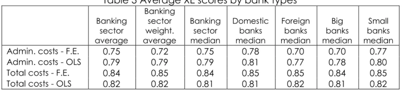
Having more detailed information on bank level allows us to compare the efficiencies between banking groups. Our results suggest that bank size does not seem to be a determinant of bank efficiency as we see no difference between bigger or smaller banks total cost efficiency. Regarding administrative cost efficiency, smaller banks are actually more efficient (Table 3). However, it is worth
0.60 0.65 0.70 0.75 0.80 0.85 0.90 0.95 1.00 1994 -1999 1996 -2001 1998 -2003 2000 -2005 2002 -2007 2004 -2009 2006 -2011 2008 -2013
XE total costs - OLS XE total costs - F.E.
XE administrative costs - OLS XE administrative costs - F.E.
0.60 0.65 0.70 0.75 0.80 0.85 0.90 0.95 1.00 1994 -1999 1996 -2001 1998 -2003 2000 -2005 2002 -2007 2004 -2009 2006 -2011 2008 -2013
XE administrative costs - OLS XE total costs - OLS
XE administrative costs - F.E. XE total costs - F.E.
mentioning that one of the advantages of XE is the fact that it is not influenced by economies of scale and therefore we are able to learn more about cost management without it being masked by bank balance sheet size. Therefore, XE concept "allows" smaller banks to be more efficient even though all the efficiency indicators from financial statements (cost to income, labour to deposits, and assets per employee) would suggest that larger banks are more efficient. Differences regarding the ownership suggest that domestic banks are more efficient on administrative level, while on the total costs level, banks are equally efficient, regardless of the ownership structure.
Table 3 Average XE scores by bank types
Banking sector average Banking sector weight. average Banking sector median Domestic banks median Foreign banks median Big banks median Small banks median
Admin. costs - F.E. 0.75 0.72 0.75 0.78 0.70 0.70 0.77 Admin. costs - OLS 0.79 0.79 0.79 0.81 0.77 0.78 0.80 Total costs - F.E. 0.84 0.85 0.84 0.85 0.85 0.84 0.85 Total costs - OLS 0.82 0.82 0.81 0.81 0.82 0.81 0.82 Source: Authors' calculation based on CNB data.
Note: OLS stands for Ordinary least squares and F.E. stands for fixed effects.
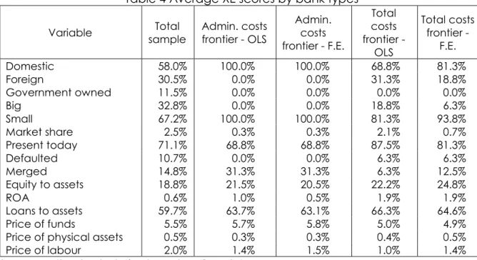
Having conducted a bank-level research allows us to describe the characteristics of the most efficient banks. Regarding the administrative costs, our frontier banks are banks with rather small average market share of just 0.3% and they are domestically owned. Two out of three most efficient banks in managing administrative costs are still present today, but even the ones that left the market, did so because they were merged with larger bank, not due to bankruptcy. In addition, banks that are most efficient in managing administrative costs have average loans to assets ratio of around 64%, which is higher, compared with the average bank. On the other hand, the ratio of equity to assets of these banks is rather high in the whole sample (around 21%). Finally, with average profitability of assets (ROA) of around 0.5-1.0 percent these banks are recording average profitability. On the other hand, banks that represent a group of most efficient bank in total costs management have a rather different characteristics. Those banks are usually somewhat bigger compared with banks that are most efficient in managing administrative costs and have a market share of around 0.7 and 2.1 percent. However, banks most efficient in managing total costs did record a couple of defaults, but the incidence was still below average. Those banks also have a relatively high loan to asset ratio as well equity to asset ratio (Table 4).
It is interesting to notice that most efficient banks in managing administrative costs usually pay a significantly higher price for funds (higher implicit interest rate on liabilities) compared with most efficient banks in managing total costs. This should not come as a surprise when we acknowledge that liabilities are the most important inputs for banks and if they pay higher price for this input, they will be motivated to increase the efficiency. As shown in the appendix (Table A2), the correlation between administrative and total cost efficiency is only moderate, at around 0.5.Finally, government owned banks did not show up on efficiency frontier in our research. However, to be fair, there are only a few government owned banks in our initial data set and there are only 95 bank year observations, which allowed for 40 XE measures.
Table 4 Average XE scores by bank types Variable Total sample Admin. costs frontier - OLS Admin. costs frontier - F.E. Total costs frontier - OLS Total costs frontier - F.E. Domestic 58.0% 100.0% 100.0% 68.8% 81.3% Foreign 30.5% 0.0% 0.0% 31.3% 18.8% Government owned 11.5% 0.0% 0.0% 0.0% 0.0% Big 32.8% 0.0% 0.0% 18.8% 6.3% Small 67.2% 100.0% 100.0% 81.3% 93.8% Market share 2.5% 0.3% 0.3% 2.1% 0.7% Present today 71.1% 68.8% 68.8% 87.5% 81.3% Defaulted 10.7% 0.0% 0.0% 6.3% 6.3% Merged 14.8% 31.3% 31.3% 6.3% 12.5% Equity to assets 18.8% 21.5% 20.5% 22.2% 24.8% ROA 0.6% 1.0% 0.5% 1.9% 1.9% Loans to assets 59.7% 63.7% 63.1% 66.3% 64.6% Price of funds 5.5% 5.7% 5.8% 5.0% 4.9% Price of physical assets 0.5% 0.3% 0.3% 0.4% 0.5% Price of labour 2.0% 1.4% 1.5% 1.0% 1.4% Source: Authors' calculation based on CNB data.
Although the differences between XE of banks seem rather small at first, a careful look at the data offers a different view. To show the impact of potential increase of efficiency on bank profitability, we calculate the potential costs savings the following way:
Cost_savings=(1-XE)*Costs, (4)
where XE is X-efficiency, and costs are administrative or total costs in absolute terms. The rationale for this formula is simple; if bank has XE score of 0.85 it means that the most efficient bank on the market would be able to offer the same services and pay the same input prices while generating only 85% of its costs. Therefore, 15% is the potential costs savings for the bank.
Figure 3 ROA with cost efficiency equal to most efficient bank Source: Authors' calculation based on CNB data.
Our results suggest that if all banks increased their efficiency in managing administrative costs to the level of the most efficient bank, costs savings could amount to 0.2% of assets on average in last twenty years. If the same simulation is applied to total costs management then the costs saving could amount to 1.2% of
assets on average. In addition, it is worth mentioning that this costs savings would be repeated each year and would significantly increase banks ROA and capital levels. Therefore, bank cost efficiency should be monitored more carefully; as costs saved are potential earnings and potential earnings are potential capital (Figure 3).
Conclusions
Although domestic and smaller banks better results in administrative costs management seems surprising, one should be aware of the fact that administrative costs represent a relatively small portion of total costs. Therefore, smaller and domestic banks that pay higher interest cost perhaps find it necessary to keep every manageable cost under control. Regarding total costs efficiency, we find no significant differences between banks regarding size or ownership from 1994-2014. Since our measure is a relative one, better than expected cost management of smaller and domestic banks could result from specific circumstances of bigger and foreign owned banks. Managing larger institutions is harder as they are involved in operations that are more complicated. In addition, banks with more market power have a higher franchise value, which they protect via more stringent credit risk management or with strategically focused activities that can appear as cost inefficiency.
Our results on bank efficiency in Croatia are comparable to other research on the matter, especially ones using trans-log cost functions and frontier analysis (DFA or SFA). Average and medial bank is relatively close to the most efficient bank, however, although it may seem that differences in cost efficiencies are small and that the potential earnings on costs are small, should all banks increase their efficiency to the level of most efficient bank, bank ROA could be increased noticeably. Moreover, even though it is not realistic to expect that all banks increase their efficiency to the frontier, the result show that further work on the issues of bank efficiency could be beneficial. This is especially obvious when we consider the fact that cost savings refer to each year, so on cumulative level significant gains for earnings could be achieved. By increasing the ROA, those savings could increase capital adequacy (providing that the earnings be retained) or owners' welfare (providing that the dividends be distributed).
While commenting on the results of all efficiency research based on frontier analysis, one has to have in mind the specificity of efficiency measure. XE shows the relative ability of a management to keep the costs, given prices and quantities of inputs, relatively close to the best cost-managing bank on the market. Therefore, the fact that smaller banks usually pay higher price for input as well as that they benefit less from the economies of scale plays no technical role with this measure. Higher than expected average XE of smaller banks could be a result of the fact that they think twice before spending money while bigger banks can act strategically or enjoy the “quiet life” of larger institution. Combined with better credit-risk management, they perhaps do not feel the pressure to worry about administrative costs that much.
Our results also suggest that depending on the scope of cost definition, efficiency can differ although we derive comparable results by using different model specification (panel OLS or panel with effects). This is important as different authors use different definition of cost as well as model specification, which makes their result less comparable. It is also worth mentioning that data truncation can play an important role in efficiency scores. In our research, we removed the banks that had a “suspicious” data in the beginning and therefore no further trimming was needed when we averaged the residuals. However, some authors run the regression first, and then trim the banks with extreme residuals. Different data truncation rules also lead
to different results as more rigorous truncating rules will reduce the differences between observed banks and efficiency scores will be closer to one.
To conclude, our results are opposite to the general impression that larger and foreign owned banks are more efficient or that banks "increased their efficiency after the financial crisis started", however they are still comparable with some earlier research based on the similar techniques. Looking at the average and weighted average scores, relative efficiency did increase after 2005-2010 but nothing to suggest some major strategic changes in the cost management practices. Going further, our research could serve as a motivation for other bank level research on Croatian banking sector. Therefore, cost inefficiencies are making the life of bank managers more comfortable, but in the same time, owners' welfare could be suffering which opens the question of agency theory in Croatian banking sector. In addition, it should be kept in mind that XE is only one of the empirically based efficiency of the individual bank. Only by calculating scale and scope efficiency as well as XE, one can have a clear picture about cost efficiency of banks.
References
1. Ariss, R. T. (2010). On the implications of market power in banking: Evidence from developing countries. Journal of banking & Finance, Vol. 34, pp. 765-775.
2. Berger, A. (1993). ’Distribution-Free’ Estimates of Efficiency in the U.S. Banking Industry and Tests of the Standard Distributional Assumptions. Journal of Productivity Analysis, Vol. 4, pp. 261-292.
3. Berger, A., Hannan T. (1998). The efficiency cost of market power in the banking industry: A test of the “quiet life” and related hypotheses, Review of Economics and Statistics, Vol. 80, pp. 454-465.
4. Berger, A., Hunter, W. C., Timme, S. G. (1993). The efficiency of financial institutions: A review and preview of research past, present and future. Journal of Banking and Finance, Vol. 17, pp. 221-249.
5. De Young, R. (1997). A Diagnostic Test for the Distribution-Free Efficiency Estimator: An Example Using U.S. Commercial Bank Data. European Journal of Operational Research, Vol. 98, pp. 243-249.
6. Farrell, M. J. (1957). The Measurement of Productive Efficiency. Journal of the Royal Statistical society, Vol. 120, pp. 253-290.
7. Hausman, J. (1978). Specification tests in econometrics. Econometrica, Vol. 46, pp. 1251-1271.
8. Huljak, I. (2015). Testing Out the "Quiet-Life" Hypothesis on Croatian Banking Sector, In Proceedings of the 5th Eastern European Economic and Social Development Conference
on Social Responsibility, Jovancai Stakic, A., Kovsca, V., Bendekovic, J., Eds., Belgrade, Serbia, May 21-22, 2015, pp. 343-353.
9. Hymer, S., Pashigan, P. (1962). Firm size and rate of growth. Journal of Political Economy, Vol. 70, pp. 556-569.
10.Jemrić, I., Vujčić, B. (2002). The Efficiency of Banks in Croatia: A Data-Envelopment Approach. Comparative Economic Studies, Vol. 44, pp. 169-193.
11.Kraft, E., Payne, J., Hofler, R. (2004). Privatization, Foreign Bank Entry, and Bank Efficiency in Croatia: A Fourier-Flexible Stochastic Frontier Analysis. Applied Economics, Vol. 38, pp. 2075-2088.
12.Kraft, E., Tirtiroglu, D. (1998). Bank Efficiency in Croatia: A Stochastic-Frontier Analysis. Journal of Comparative Economics, Vol. 26, pp. 286-300.
13.Leibenstein, H. (1966). Allocative Efficiency vs. "X-efficiency". The American Economic review, Vol. 56, pp. 392-415.
About the author
Ivan Huljak, PhD, received in 2004 the Bachelor’s degree in Finance and in 2010 the
Master of Science degree in Corporate Finance at the Faculty of Economics and Business, University of Zagreb. In 2014, he received his PhD in the field of banking and industrial organisation with thesis: "The net effect of bank market power in CEE countries” at Faculty of Economics, University of Split. During his work in Croatian National Bank, he attended various seminars and workshops and presented his work on international conferences on the topics of financial stability. The author currently works as a Senior Advisor in Financial Stability Department at Croatian National Bank and his field of interest is banking, financial stability and industrial organisation. The author can be contacted at ivan.huljak@hnb.hr.
Appendix
Table A1 Trans-log function results
Administrative costs Total costs
OLS F.E. OLS F.E.
ln(y1) 0.39 *** 0.36 *** 0.98 *** 0.89 *** ln(y2) 0.41 *** 0.31 *** 0.46 *** 0.13 ln(y3) 0.06 0.01 -0.22 * 0.09 ln(w1) -0.14 -0.08 0.05 0.27 * ln(w2) 0.67 *** 0.37 *** 0.71 *** 0.49 *** ln(w3) 0.21 0.17 0.37 0.57 ** ln_y1*ln_y1/2 0.19 *** 0.16 *** 0.23 *** 0.16 *** ln_y2*ln_y2/2 0.19 *** 0.17 *** 0.18 *** 0.16 *** ln_y3*ln_y3/2 -0.02 * -0.06 *** 0.08 *** 0.06 *** ln_w1*ln_w1/2 0.07 *** 0.04 0.08 ** 0.12 *** ln_w2*ln_w2/2 0.09 *** 0.07 *** 0.05 *** 0.04 *** ln_w3*ln_w3/2 0.23 *** 0.26 *** 0.29 *** 0.25 *** ln_y1*ln_y2/2 -0.36 *** -0.32 *** -0.37 *** -0.25 *** ln_y1*ln_y3/2 0.02 0.07 *** -0.12 *** -0.06 * ln_y2*ln_y3/2 -0.02 0.01 -0.02 -0.08 *** ln_w1*ln_w2/2 0.02 0.02 0.08 ** 0.04 ln_w1*ln_w3/2 -0.04 -0.06 -0.10 0.01 ln_w2*ln_w3/2 -0.19 *** -0.22 *** -0.17 *** -0.17 *** ln_y1*ln_w1/2 -0.06 -0.09 ** 0.06 0.11 ** ln_y1*ln_w2 -0.07 *** -0.02 -0.09 *** -0.05 ** ln_y1*ln_w3 0.17 *** 0.12 *** 0.23 *** 0.17 *** ln_y2*ln_w1 0.06 *** 0.05 *** 0.03 0.01 ln_y2*ln_w2 0.01 -0.01 0.02 0.00 ln_y2*ln_w3 -0.02 -0.01 -0.08 *** -0.07 ** ln_y3*ln_w1 -0.01 0.01 -0.02 -0.03 ** ln_y3*ln_w2 0.06 *** 0.02 ** 0.04 *** 0.03 * ln_y3*ln_w3 -0.13 *** -0.06 *** -0.17 *** -0.10 *** _cons 2.74 *** 3.05 *** 0.83 2.12 *** R-square 0.99 0.99 0.98 0.98 N. of obs. 814 814 812 812 Source: Authors' calculation based on CNB data,
Note: * p<0.05, ** p<0.01, *** p<0.001, OLS stands for Ordinary least squares and F.E. stands for fixed effects.
Table A2 XE scores correlates
costs - F.E Admin. costs - OLS Admin. Total costs - F.E. Total costs - OLS
Admin. costs - F.E 1.00
Admin costs - OLS 0.90 1.00 Total costs - F.E. 0.53 0.50 1.00 Total costs - OLS 0.46 0.48 0.87 1.00 Source: Authors' calculation based on CNB data.
Note: OLS stands for Ordinary least squares and F.E. stands for fixed effects. Table A3 XE results for administrative costs Banking sector average Banking sector weighted average Banking sector median Domestic banks median Foreign banks median Big banks median Small banks median OLS 1994-1999 0.76 0.76 0.76 0.76 0.70 0.78 0.75 1995-2000 0.77 0.77 0.77 0.78 0.73 0.77 0.77 1996-2001 0.80 0.77 0.80 0.82 0.78 0.78 0.81 1997-2002 0.79 0.78 0.81 0.81 0.79 0.78 0.82 1998-2003 0.81 0.79 0.83 0.84 0.78 0.78 0.84 1999-2004 0.77 0.74 0.77 0.78 0.72 0.71 0.78 2000-2005 0.81 0.78 0.80 0.84 0.77 0.77 0.81 2001-2006 0.82 0.79 0.81 0.85 0.79 0.78 0.82 2002-2007 0.80 0.79 0.80 0.83 0.78 0.79 0.82 2003-2008 0.80 0.79 0.79 0.83 0.77 0.78 0.82 2004-2009 0.80 0.81 0.80 0.83 0.78 0.80 0.82 2005-2010 0.80 0.81 0.80 0.81 0.78 0.80 0.81 2006-2011 0.79 0.81 0.78 0.79 0.77 0.78 0.78 2007-2012 0.78 0.80 0.77 0.79 0.76 0.78 0.77 2008-2013 0.78 0.81 0.77 0.79 0.76 0.78 0.77 2009-2014 0.79 0.82 0.78 0.77 0.78 0.78 0.78 F.E. 1994-1999 0.73 0.71 0.75 0.76 0.67 0.72 0.75 1995-2000 0.74 0.72 0.75 0.78 0.69 0.74 0.77 1996-2001 0.77 0.72 0.78 0.80 0.72 0.73 0.80 1997-2002 0.76 0.73 0.78 0.81 0.73 0.73 0.80 1998-2003 0.79 0.74 0.80 0.83 0.73 0.73 0.82 1999-2004 0.75 0.69 0.74 0.80 0.67 0.67 0.78 2000-2005 0.77 0.72 0.76 0.82 0.71 0.69 0.80 2001-2006 0.75 0.70 0.74 0.81 0.70 0.69 0.78 2002-2007 0.74 0.70 0.73 0.79 0.69 0.68 0.77 2003-2008 0.74 0.70 0.74 0.78 0.68 0.68 0.77 2004-2009 0.74 0.71 0.74 0.77 0.70 0.70 0.76 2005-2010 0.75 0.72 0.74 0.78 0.70 0.70 0.77 2006-2011 0.74 0.72 0.74 0.76 0.70 0.70 0.75 2007-2012 0.74 0.72 0.72 0.76 0.69 0.69 0.74 2008-2013 0.73 0.72 0.72 0.77 0.70 0.69 0.75 2009-2014 0.74 0.72 0.73 0.72 0.74 0.69 0.75 Source: Authors' calculation based on CNB data.
Table A4 XE results for total costs Banking sector average Banking sector weighted average Banking sector median Domestic banks median Foreign banks median Big banks median Small banks median OLS 1994-1999 0.81 0.84 0.79 0.78 0.89 0.79 0.80 1995-2000 0.86 0.89 0.86 0.84 0.87 0.86 0.85 1996-2001 0.88 0.90 0.89 0.86 0.93 0.88 0.89 1997-2002 0.87 0.90 0.88 0.85 0.92 0.92 0.85 1998-2003 0.79 0.80 0.78 0.77 0.78 0.80 0.77 1999-2004 0.72 0.72 0.71 0.70 0.70 0.70 0.71 2000-2005 0.78 0.78 0.77 0.77 0.78 0.76 0.77 2001-2006 0.80 0.80 0.80 0.80 0.81 0.78 0.80 2002-2007 0.79 0.80 0.80 0.80 0.80 0.79 0.80 2003-2008 0.79 0.79 0.80 0.81 0.79 0.79 0.81 2004-2009 0.78 0.78 0.79 0.80 0.79 0.78 0.81 2005-2010 0.79 0.78 0.79 0.79 0.79 0.78 0.79 2006-2011 0.82 0.81 0.81 0.82 0.80 0.80 0.81 2007-2012 0.84 0.84 0.83 0.87 0.82 0.83 0.84 2008-2013 0.86 0.85 0.85 0.87 0.85 0.85 0.87 2009-2014 0.88 0.86 0.85 0.86 0.85 0.84 0.87 F.E. 1994-1999 0.83 0.84 0.83 0.82 0.89 0.82 0.83 1995-2000 0.85 0.88 0.87 0.86 0.85 0.85 0.87 1996-2001 0.84 0.85 0.86 0.85 0.88 0.86 0.86 1997-2002 0.85 0.87 0.87 0.85 0.88 0.88 0.83 1998-2003 0.80 0.81 0.80 0.80 0.80 0.81 0.79 1999-2004 0.80 0.80 0.79 0.80 0.78 0.79 0.79 2000-2005 0.85 0.86 0.85 0.84 0.86 0.84 0.85 2001-2006 0.86 0.87 0.87 0.87 0.87 0.85 0.87 2002-2007 0.84 0.85 0.85 0.85 0.85 0.85 0.85 2003-2008 0.84 0.85 0.85 0.85 0.85 0.84 0.85 2004-2009 0.82 0.83 0.84 0.84 0.84 0.84 0.84 2005-2010 0.82 0.82 0.82 0.81 0.82 0.82 0.82 2006-2011 0.85 0.84 0.84 0.85 0.84 0.85 0.83 2007-2012 0.88 0.87 0.87 0.91 0.86 0.86 0.88 2008-2013 0.88 0.87 0.86 0.89 0.86 0.86 0.89 2009-2014 0.87 0.85 0.84 0.85 0.84 0.84 0.88 Source: Authors' calculation based on CNB data.
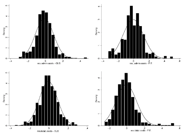
Figure A1 Averaged residuals histograms Source: Authors' calculation based on CNB data.
Figure A2 XE histograms Source: Authors' calculation based on CNB data.