No. 2005–108
TRIMMED LIKELIHOOD-BASED ESTIMATION IN BINARY
REGRESSION MODELS
%\3DYHOýtåHN
September 2005
Trimmed likelihood-based estimation in binary
regression models
Pavel ˇC´ıˇzek
Abstract: The binary-choice regression models such as probit and logit are typically estimated by the maximum likelihood method. To improve its robustness, various M-estimation based procedures were proposed, which however require bias corrections to achieve consistency and their resistance to outliers is relatively low. On the contrary, traditional high-breakdown point methods such as maximum trimmed likelihood are not applicable since they induce the separation of data and thus non-identification of estimates by trimming observations. We propose a new robust estimator of binary-choice models based on a maximum symmetrically trimmed likelihood estimator. It is proved to be identified and consistent, and additionally, it does not create separation in the space of explanatory variables as the existing maximum trimmed likelihood. We also discuss asymptotic and robust properties of the proposed method and compare all methods by means of Monte Carlo simulations.
Zusammenfassung: Regressionsmodelle mit diskreten abh¨angigen Vari-ablen, z.B. probit und logit, werden typischerweise durch das Maximum-Likelihood Prinzip gesch¨atzt. Wegen ihrer niedrigeren Robustheit wurden verschiedene M-Sch¨atzer von bin¨aren Modellen vorgeschlagen, die aber auch asymptotisch auf Verzerrung korigiert werden m¨ussen und nicht beson-ders robust sind. Andererseits sind hoch-robuste Methoden der linearen Re-gression, z.B. die Maximum-Trimmed-Likelihood Methode, nicht anwend-bar, weil sie nicht identifiziert werden k¨onnen. Hier konstruieren wir einen robusten Sch¨atzer f¨ur bin¨are Regressionsmodelle, der auf eine symmetrisch beschneidete Maximum-Likelihood Methode basiert. Der Sch¨atzer ist be-wiesen, identifiziert und konzistent zu sein. Wir diskutieren auch seine ro-busten Eigenschaften und vergleichen ihm mit anderen bekannten roro-busten Methoden durch die Monte Carlo Simulationen.
Keywords: binary-choice regression, maximum likelihood, robust estima-tion, trimming.
JEL codes: C13, C25
1 Introduction
The binary-choice regression models such as probit and logit are used to describe the effect of explanatory variables xi ∈ Rp on a binary response variable yi ∈ {0,1}, i =
1, . . . , n:
P(yi = 1|xi) = F(x>i β), (1)
where F is a known link function (e.g., the standard normal distribution function Φ
unknown parameters. Applications include estimating probability of a firm’s bankruptcy and modeling decisions to work, retire, or have children.
Model (1) is typically estimated by the maximum likelihood estimator (MLE), which is defined by ˆ βM LE = arg max β n X i=1 l(yi, xi;β), (2)
where the likelihood contributions are
l(yi, xi;β) = yilnF(x>i β) + (1−yi) ln{1−F(x>i β)}. (3)
This estimator is identified only if the two parts of data given by the values of the re-sponse variable,{xi|yi = 1}and{xi|yi = 0}, are not separated in the space of
explana-tory variables (Albert and Anderson, 1984). MLE is also asymptotically normal and ef-ficient, but it can behave rather poorly if data are contaminated (Croux et al., 2002); for example, if data contain misclassified observations with extreme values of explanatory variables or exhibit an uknown form of heteroscedasticity. Several robust alternatives have been therefore proposed and studied.
In this context, traditional robust (high-breakdown point) methods such as nonlinear least trimmed squares (LTS; Stromberg and Ruppert, 1992; ˇC´ıˇzek, 2005) and maxi-mum trimmed likelihood (MTLE; M¨uller and Neykov, 2003) are not generally applica-ble since, by trimming observations, they induce the separation of data and thus non-identification of estimates. The only exception are data sets containing large strata, where the number of observations at any observed point xi grows with sample size
(Christman, 1994). Therefore, most recent results rely on M-estimation to achieve ro-bustness: the likelihood contribution functionl(y, x;β)is replaced by another function φ(y, x;β), which is bounded and possibly contains “weighting” partw(x;γ)depending only on the explanatory variablesxand some nuisance parametersγ. Recent examples include Copas (1988), Carroll and Pederson (1993), Bianco and Yohai (1996), Kordza-khia et al. (2001), Croux and Haesbroeck (2003), and Gervini (2005).
The described approach based on M-estimation has in many cases two important de-ficiencies: asymptotic bias causing inconsistency and relatively low robustness. First, the inconsistency of these estimators was noted, for example, by Carroll and Pederson (1993) and can be remedied only by finding and including a bias-correction term into the objective function of a respective estimator (see Bianco and Yohai, 1996, for instance). A disadvantage stemming from this approach lies in low flexibility of such procedures: consistent robust estimators are often designed for logit and their adaptation to other (more flexible) models like in Hausmann et al. (1998) can require redesign of the estima-tion procedure. Next, the low robustness of M-estimators to misclassified observaestima-tions with extreme value of explanatory variables was observed and remedied, for example, by Croux and Haesbroeck (2003) and Gervini (2005). A typical remedy unfortunately relies on simple downweighting of distant observations in the space of explanatory vari-ables irrespective to whether they are misspecified or not and to what influence they have on the model.
We propose a new robust estimator of binary-choice models. Even though it relies on a symmetrically trimmed form of maximum likelihood estimator, it is proved to be
identified and consistent in a very general setting. Thus, it does not exhibit any asymp-totical bias, it is widely applicable, and additionally, it does not create separation in the space of explanatory variables as LTS and MTLE do. In the rest of this paper, we first identify the source of non-identification of MTLE caused by trimming and motivate a solution in Section 2. Further, we discuss conditions under which the proposed solution is consistent in Section 3 and we mention some important robust properties in Section 4. Finally, we compare the proposed method with some existing solutions using Monte Carlo simulations in Section 5.
2 Identification
Let us first demonstrate why the classical trimmed estimators such as MTLE are not correctly identified in model (1), which will later motivate our proposal. Maximum trimmed likelihood estimator (MTLE) is defined by
ˆ
β(M T LE,hn) = arg max
β∈B n X j=1 lnl(xi, yi;β)·I ³ lnl(xi, yi;β)≥lnl[n−hn+1](xi, yi;β) ´ , (4) wherel[j](xi, yi;β)denotes thejth order statistics of likelihood contributionsl(xi, yi;β),
i = 1, . . . , n, and hn ∈ {[n/2] + 1, . . . , n} is the trimming constant. The trimming
constant determines how many observations hn are kept in the objective function and
how many observations n −hn are excluded from estimation to protect the estimator
against errors in data. The rule used for trimming in (4) is described by the indicator function
I³lnl(xi, yi;β)≥lnl[n−hn+1](xi, yi;β)
´
and keeps in the objective function thehn “most likely” observations, that is,hn
obser-vations with the largest likelihood.
If MTLE as an extremum estimator is identified, the expectation of its objective function (see ˇC´ıˇzek, 2004, for derivation)
IC(β) = E[lnl(xi, yi;β)·I(lnl(xi, yi;β)≥qλ(β))]
has to have a maximum at the true valueβ0of parameter vectorβ;qλ(β)refers here to the
λ-quantile of the distribution oflnl(xi, yi;β), whereλ= 1−limn→∞hn/n. Therefore,
if the MTLE estimator is identified, the first-order conditions∂IC(β)/∂β = 0 should hold atβ0.
To verify the first-order conditions, letf denote the density function corresponding toF in (1) and note that (3) and the law of iterated expectation implies (see ˇC´ıˇzek, 2004, for details) ∂IC(β0) ∂β =E "( yif(x>i β0) F(x> i β0) xi− (1−yi)f(x>i β0) 1−F(x> i β0) xi ) I(lnl(xi, yi;β0)≥qλ(β0)) # =Ex " P(yi = 1|xi) f(x> i β0) F(x> i β0) xiI(lnl(xi,1;β0)≥qλ(β0)) # (5)
−Ex " P(yi = 0|xi) f(x> i β0) 1−F(x> i β0) xiI(lnl(xi,0;β0)≥qλ(β0)) # (6) =Ex n f(x>i β0)xi h I³lnF(x>i β0)≥qλ(β0) ´ −I³ln{1−F(xi>β0)} ≥qλ(β0) ´io . Hence, the first-order condition is satisfied in general only if it holds for all possible values of the random vectorxthat
I³lnF(x>β 0)≥qλ(β0) ´ =I³ln{1−F(x>β 0)} ≥qλ(β0) ´ ; (7)
that is, only in the case of the MLE objective function with no trimming,qλ(β0) =−∞
andλ = 0, and in the case of the constantly zero objective function, qλ(β0) = 0 and
λ= 1. Thus, the MTLE estimator is not identified at anyλ∈(0,1).
On the other hand, this derivation hints that the necessary identification condition would hold if the rule used for trimming observations has the same form both in (5) and (6). In other words, the first-order condition would hold if the trimming rule is independent of the valueyi, which motivates the following proposal: instead of the
log-likelihood contributions, let us compare the minimum of the log-log-likelihood contributions taken over all possible values ofyi ∈ {0,1}and trim observations with low values of
minnlnF(x>β0),ln[1−F(x>β0)]
o
.
The resultingmaximum symmetrically trimmed likelihood estimator (MSTLE) is then defined by
ˆ
β(M ST LE,hn) = arg max
β∈B n X j=1 lnl(xi, yi;β)·I ³ r(xi, yi;β)≥r[n−hn+1](xi, yi;β) ´ , (8) wherer(xi, yi;β) = min n lnF(x>β 0),ln[1−F(x>β0)] o
.The first-order conditions for the local identification of the parameter estimates in model (1) are then satisfied as fol-lows from (5)–(6), whereqλ(β)has to refer now to theλ-quantile of the distributionGβ
ofr(xi, yi;β). Complete verification of both the first-order and second-order
identifica-tion condiidentifica-tions is done in ˇC´ıˇzek (2001).
3 Asymptotic properties
The maximum symmetrically trimmed likelihood estimator defined by (8) can be iden-tified in binary-choice models as argued in Section 2. In this section, we demonstrate that it is also consistent under rather general conditions, and therefore, does not require any asymptotic bias correction as many existing M-estimators. We first discuss the suf-ficient conditions for the consistency of MSTLE and provide the corresponding theo-retical result. Later, we mention additional conditions that might be necessary to prove √
n-consistency and asymptotic normality of this estimator.
The assumptions sufficient for the MSTLE consistency form three groups: distri-butional assumptions D, assumptions F concerning the MSTLE objective function, and identification assumptions I.
D Let random variables{yi, xi}i∈N form an independent and identically distributed
sequence of random vectors with finite second moments. Further, assume that the distribution functionGβ ofr(xi, yi;β)is absolutely continuous with densitygβfor
anyβ∈B and that it holds formG = infβ∈Bqλ(β)andMG = supβ∈Bqλ(β)that
Mgg = sup β∈B sup z∈(mG−δ,MG+δ) gβ(z)<∞ (9) and mgg= inf β∈Bz∈inf(−δ,δ)gβ(qλ(β) +z)>0 (10) for someδ >0.
F Letl(xi, yi;β)be continuous (uniformly over any compact subset of the support
of(xi, yi)) inβ ∈ B. Further, let expectation Esupβ∈B|l(xi, yi;β)|1+δ exist and
be finite for someδ >0.
I Let B be a compact parametric space, and for any ε > 0 andU(β0, ε)such that
B\U(β0, ε)is compact, letα(ε)>0exist such that it holds min
β∈B\U(β0,ε)
E[l(xi, yi;β)·I(r(xi, yi;β)≤qλ(β))]
−E[l(xi, yi;β0)·I(r(xi, yi;β0)≤qλ(β0))] > α(ε).
Whereas some assumptions are well-known from the literature, such as the existence of the finite first or second moments of random variables and the identification assumptions I mentioned already in Section 2, there is one less usual regularity assumption. It stems from the generality of the model specification, which does not require anything but con-tinuity of the link function F. Assumptions (9) and (10) formalize two things: (i) the density functiongβ has to be bounded uniformly inβ ∈ B, which prevents distribution
Gβ to be arbitrarily close to a discrete one within the parametric space B; and (ii) the
density functiongβ has to be positive in a neighborhood of theλ-quantile ofGβ, that is,
around the chosen “trimming” point of ther(xi, yi;β)distribution. This type of
assump-tions is standard in literature on asymptotics of trimmed estimators, see ˇC´ıˇzek (2005) for more details.
Under these conditions, it is possible to prove the following result.
Theorem 1 Let Assumptions D, F, and I hold. Then the MSTLE estimatorβˆ(M ST LE,hn)
is weakly consistent, that is,βˆ(M ST LE,hn) →β
0in probability asn→+∞.
Proof:The theorem is a direct consequence of ˇC´ıˇzek (2004, Theorem 2). Q.E.D.
As shown in ˇC´ıˇzek (2004), this result can be extended to derive the√n-rate of con-vergence of the MSTLE estimator if additional assumptions regarding differentiability of l(xi, yi;β)and some other regularity assumptions are satisfied. Even though it is seems
that the same conditions should be sufficient for proving the asymptotic normality of MSTLE, no such result is currently available.
4 Robust properties
After proving that MSTLE is a valid estimator of model (1), we concetrate now on the robustness of the proposed solution. Traditionally, the global robustness of an estimator is measured by the breakdown point. It can be defined as the largest fraction(m−1)/n of sample observations that can be arbitrarily changed without making the estimator “useless” (and naturally, changing then m observations in a right way can make the estimator “useless”), that is, without making estimator a constant, non-random function (Genton and Lucas, 2003).
One of the first results concerning the breakdown point in the binary-choice regres-sion is by Christmann (1994), who shows that the breakdown pointε∗
nof most estimators
is design (sample) specific, ε∗ n≤ 1 n " min ( n X i=1 yi, n− n X i=1 yi ) −1 # ,
and depends on the relative number of observations with responsesyi = 1andyi = 0,
respectively. The following theorem complements this general result by providing upper bounds for the breakdown point of MSTLE. They are not sample specific and indicate that, contrary to linear regression, trimming more observations does not necessarily re-sult in a higher breakdown point.
Theorem 2 The breakdown point of MSTLE estimator (8) with trimminghn ∈ {[n/2] +
1, . . . , n}is in model (1) bounded byε∗
n≤[hn/2]/n.
Proof:Consider a sample(xi, yi)ni=1and define a contaminated sample(x∗i, y∗i) = (xi, yi)
fori= 1, . . . , n−[hn/2]−1and(x∗n−i, yn∗−i) = (xi,1−yi)fori = 1, . . . ,[hn/2] + 1.
Thus, we changed only[hn/2]+1observations so that the new sample contains[hn/2]+1
pairs of observation with identical valuesxi and complementary valuesyi. The MSTLE
estimator applied to(x∗
i, yi∗)trims all non-paired observations and results inβˆ = 0
be-cause both the joint likelihood and trimming ruler(x∗
i, yi∗;β) = ln(1/2) of all paired
observations reach its maximum atβ = 0. Thus, all other (non-paired) observations are trimmed from the objective function. Q.E.D.
On the one hand, the breakdown point is thus bounded by(n−hn)/nbecausen−hn
determines the number of observations that can be trimmed from the objective function. On the other hand, misspecification of the values of the dependent variable described in Theorem 2 imposes another bound [hn/2]/n. Consequently, trimming constant hn
should not be chosen smaller thanhn = [(2n)/3], which follows from equating the two
bounds, (n −hn)/n = hn/(2n), and indicatesε∗n ≤ 1/3. Due to further data-specific
limits on the breakdown point (as in Christmann, 1994),hn≥[(3n)/4]will probably be
a realistic choice in applications.
Finally, note the breakdown point describes a method’s behavior only in the extreme situation of its failure. The influence of a point-mass contamination at various locations on the estimation can be however quantified by the so-called bias curve. Because it is difficult to obtain an analytic expression for the bias curve, we will evaluate it by means of Monte Carlo simulations in Section 5 and compare it with bias curves of other existing estimators.
5 Simulation study
To compare the performance of various methods for estimating binary-choice regression models in finite samples, Monte Carlo simulations are used. In this section, we compare the proposed MSTLE method with MLE and the Bianco and Yohai (1996) estimator (BYE), which is based on a bias-corrected M-estimator and was implemented by Croux and Haesbroeck (2003). We also consider weighted forms of MLE and BYE based on weights defined by
W wi =I(RDi2 ≤χ2p,0.975), whereχ2p,0.975denotes the 97.5% quantile ofχ2
distribu-tion with p degrees of freedom and RDi represents the Mahalanobis distance of
theith observation based on the robust MCD estimate of location and covariance (see Croux and Haesbroeck, 2003, for details);
WT wi = min{c,exp(r(xi, yi;β))}= min
n
c, F(x>β
0),1−F(x>β0)
o
, where r(xi, yi;β)is the rule used for trimming in (8) andc= 0.1, for instance.
The first choice defines weights just by the position of observations in the space of ex-planatory variables and downweights all distant observations. It is frequently used in the literature (e.g., Croux and Haesbroeck, 2003; Gervini, 2005). The latter choice relies on the initial robust fit by MSTLE and downweights only observations with low values of trimming ruler(xi, yi;β). The precise choice of weights is arbitrary at this moment and
optimal weighting scheme has to be further researched.
As BYE is currently implemented only for logit, we compare all methods using a logistic model as a data-generating process. Specifically, we generate two explanatory variablesx1, x2 ∼ N(0,1), and for a given parameter vector b = (b0, b1, b2), we define
y = I(b0 +b1x1 +b2x2 +ε ≥ 0), where ε ∼ Λ(0,1) (N(µ, σ) and Λ(µ, s) refer
to the Gaussian and logistic distributions, respectively). If a generated data set is not further modified, we refer to it as CLEAN. Next, to examine robust properties of all estimators, we also use contaminated data: a given fractionα ∈ (0,1)of observations is shifted by (∆1,∆2) ∈ R2 and misclassified, which corresponds to transformations
x∗
1 = x1 + ∆1, x∗2 = x2 + ∆2, andy∗ = I(b0+b1x∗1 +b2x∗2 < 0). Such data sets are
referred to as OUTLIERS(α;∆1,∆2). Finally, to estimate bias curves of all estimators,
we use data with a point-mass contamination: a given fractionα∈(0,1)of observations is set to(∆1,∆2)and misclassified, which corresponds to setting x∗1 = ∆1, x∗2 = ∆2,
andy∗ =I(b
0+b1x∗1+b2x∗2 <0). These data sets are denoted POINTCONT(α;∆1,∆2).
Let us note that the results discussed in this section are obtained for sample sizes n = 100 observations, trimming constanthn = 75, and 500 simulations. Although we
also experimented with larger sample sizes, it seems that the performance of MSTLE at smaller samples is worse relative to other methods than at larger samples, and therefore, we present less favorable results for MSTLE.
5.1 Bias curve
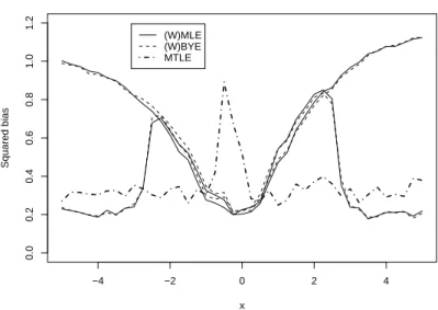
To quantify influence of data contamination on estimation, we evaluate the bias curves of all discussed estimators in the logistic model with parametersb = (0.5,1.0,0.0)with
−4 −2 0 2 4 0.0 0.2 0.4 0.6 0.8 1.0 1.2
Absolute bias curve, 10% contamination
x
Squared bias
(W)MLE (W)BYE MTLE
Figure 1: Bias curves of the (W)MLE (solid curves), (W)BYE (dashed curves), and MSTLE (dot-dashed curve) estimators.
10% point-mass contamination at points from interval(−5,5). This amount to simulat-ing and estimatsimulat-ing data POINTCONT(0.10;x,0) for x ∈ (−5,5), which is done here using an equidistant grid with step 0.25. Note that contamination around x = −0.50
causes only misclassification, not real outliers.
The results are summarized on Figure 1, which depicts the squared bias of each es-timator as a function of contamination pointx. First, the standard result indicating low robustness of MLE and BYE is demonstrated here by bias steadily increasing with the in-creasing distance of contamination pointxfrom the origin. The weighted forms of these estimators, WMLE and WBYE, behave similarly to MLE and BYE forx2 ≤ χ2
1,0.975,
but are not influenced by the contamination forx2 > χ2
1,0.975because the contaminated
observations have then weights equal to zero. The bias curve of MSTLE looks rather differently. On the one hand, it exhibits a comparatively large bias for contamination close to the origin because it uses just pre-specifiedhn = 75observations and trims the
remaining ones, that is, good ones in this case. On the other hand, the bias of MSTLE is rather small and practically constant for allx 6∈ (−1,0), that is, when data contain real outliers. Note that whereas MSTLE performs equally well both in samples with moder-ate and large outliers, WMLE and WBYE perform well only if outliers are far enough from the correct observations.
5.2 Estimation under contamination
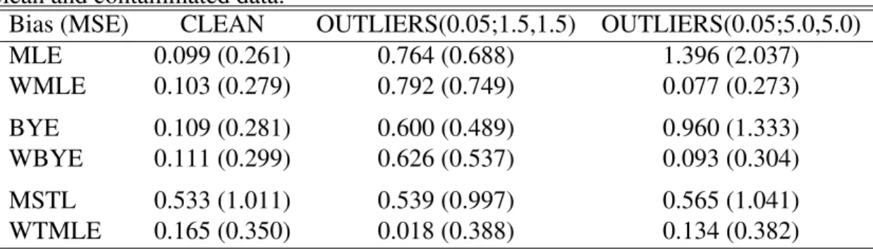
The performance of all methods is now analyzed both under clean and contaminated data sets generated from the logistic model withb= (0.5,1.0,−1.0). Employed data are CLEAN, OUTLIERS(0.05; 1.5,−1.5), and OUTLIERS(0.05; 5.0,−5.0) and the
con-Table 1: Bias and mean squared error (MSE) of (W)MLE, (W)BYE, and MSTLE for clean and contaminated data.
Bias (MSE) CLEAN OUTLIERS(0.05;1.5,1.5) OUTLIERS(0.05;5.0,5.0) MLE 0.099 (0.261) 0.764 (0.688) 1.396 (2.037) WMLE 0.103 (0.279) 0.792 (0.749) 0.077 (0.273) BYE 0.109 (0.281) 0.600 (0.489) 0.960 (1.333) WBYE 0.111 (0.299) 0.626 (0.537) 0.093 (0.304) MSTL 0.533 (1.011) 0.539 (0.997) 0.565 (1.041) WTMLE 0.165 (0.350) 0.018 (0.388) 0.134 (0.382)
tamination level is thus 5%. The absolute value of bias and mean squared error (MSE) for each methods is recorded in Table 1.
First, very high sensitivity of MLE and BYE to outliers is again clearly visible, even though BYE is sligthly less affected by contamination. The corresponding weighted versions, WMLE and WBYE, perform rather well in the case of clean data and data with distant outliers, which can be easily detected and downweighted. Both weighted methods however fail to withstand contaminated data if outliers are not too far from the rest of data. On the contrary, the results of the proposed MSTLE method are practically unaffected by contamination, but are very imprecise; the MSE of MSTLE for clean data is almost four times higher than the MSE of MLE. This well-known inefficiency of trimmed estimators can be overcome by using them only as an initial robust estimator for a more efficient method. In our case, we use MSTLE to construct weights for MLE. The resulting WTMLE estimator is rather close to the performance of existing robust methods for clean data, but is not significantly influenced by the moderate and large outliers.
6 Conclusion
The maximum symmetrically trimmed likelihood estimator proposed in this paper is shown to be applicable in general binary-choice models, consistent, and robust to various kinds of contamination. The combination of these properties is not currently matched by any existing robust method. On the other hand, trimming of observations leads to an inevitable loss of efficiency, which can be however remedied to a large extent by using MSTLE as an initial estimator for weighted MLE. The optimal choice of weights stays as a topic for further research. Similarly, the bias curve of MSTLE indicates that a combination with models accounting for data misspecification (Hausmann et al., 1998) could be beneficial and should be further investigated.
Address:Tilburg University, Department of Econometrics & OR, Room B 616; P.O. Box 90153, 5000 LE Tilburg, The Netherlands.
References
A. Albert and J. A. Anderson (1984) On the existence of maximum likelihood estimates in logistic regression models.Biometrika71, 1–10.
A. M. Bianco and V. J. Yohai (1996) Robust estimation in the logistic regression model. In H. Rieder (ed.) Robust statistics, data analysis, and computer intensive meth-ods, Lecture notes in statistics 109, Springer, New York, 17–34.
R. J. Carroll and S. Pederson (1993) On robustness in the logistic regression model. Journal of Royal Statistical Society, Ser. B55, 693–706.
A. Christmann (1994) Least median of weighted squares in logistic regression with large strata.Biometrika81, 413–417.
P. ˇC´ıˇzek (2001) Robust estimation in nonlinear regression and limited dependent variable models. CERGE-EI Discussion Paper 189/2001, Charles University, Prague. P. ˇC´ıˇzek (2004) General trimmed estimation: robust approach to nonlinear and limited
dependent variable models. CentER Discussion Paper 130/2004, Tilburg Univer-sity, Tilburg.
P. ˇC´ıˇzek (2005) Least trimmed squares in nonlinear regression under dependence. Jour-nal of Statistical Planning & Inference, to appear.
J. B. Copas (1988) Binary regression models for contamination data.Journal of Royal Statistical Society, Ser. B50, 225–265.
C. Croux, C. Flandre, and G. Haesbroeck (2002) The breakdown behavior of the maxi-mum likelihood estimator in the logistic regression model.Statistics & Probability Letters60, 377–386.
C. Croux and G. Haesbroeck (2003) Implementing the Bianco and Yohai estimator for logistic regression.Computational Statistics & Data Analysis44, 273–295. M. G. Genton and A. Lucas (2003) Comprehensive definitions of breakdown points for
independent and dependent observations.Journal of Royal Statistical Society, Ser. B65, 81–94.
D. Gervini (2005) Robust adaptive estimators for binary regression models.Journal of Statistical Planning and Inference131, 297–311.
J. A. Hausman, J. Abrevaya, and F. M. Scott-Morton (1998) Misclassification of the de-pendent variable in a discrete-response setting.Journal of Econometrics87, 239– 269.
N. Kordzakhia, G. D. Mishra, and L. Reiersølmoen (2001) Robust estimation in the logistic regression model.Journal of Statistical Planning and Inference98, 211– 223.
C. H. M¨uller and N. M. Neykov (2003) Breakdown points of trimmed likelihood esti-mators and related estiesti-mators in generalized linear models. Journal of Statistical Planning and Inference116, 503–519.
A. J. Stromberg and D. Ruppert (1992) Breakdown in nonlinear regression.Journal of American Statistical Association87, 991–997.