Stephen, Bruce and Mutanen, Antti and Galloway, Stuart and Burt,
Graeme and Jarventausta, Pertti (2014) Enhanced load profiling for
residential network customers. IEEE Transactions on Power Delivery, 29
(1). pp. 88-96. ISSN 0885-8977 ,
http://dx.doi.org/10.1109/TPWRD.2013.2287032
This version is available at http://strathprints.strath.ac.uk/43426/
Strathprints is designed to allow users to access the research output of the University of Strathclyde. Unless otherwise explicitly stated on the manuscript, Copyright © and Moral Rights for the papers on this site are retained by the individual authors and/or other copyright owners. Please check the manuscript for details of any other licences that may have been applied. You may not engage in further distribution of the material for any profitmaking activities or any commercial gain. You may freely distribute both the url (http://strathprints.strath.ac.uk/) and the content of this paper for research or private study, educational, or not-for-profit purposes without prior permission or charge.
Any correspondence concerning this service should be sent to Strathprints administrator:
Abstract— Anticipating load characteristics on low voltage
circuits is an area of increased concern for Distribution Network Operators with uncertainty stemming primarily from the validity of domestic load profiles. Identifying customer behavior makeup on a LV feeder ascertains the thermal and voltage constraints imposed on the network infrastructure; modeling this highly dynamic behavior requires a means of accommodating noise incurred through variations in lifestyle and meteorological conditions. Increased penetration of distributed generation may further worsen this situation with the risk of reversed power flows on a network with no transformer automation. Smart Meter roll-out is opening up the previously obscured view of domestic electricity use by providing high resolution advance data; while in most cases this is provided historically, rather than real-time, it permits a level of detail that could not have previously been achieved. Generating a data driven profile of domestic energy use would add to the accuracy of the monitoring and configuration activities undertaken by DNOs at LV level and higher which would afford greater realism than static load profiles that are in existing use. In this paper, a linear Gaussian load profile is developed that allows stratification to a finer level of detail while preserving a deterministic representation.
Index Terms—Automatic meter reading (AMR), domestic load
profiling, energy demand, low voltage networks
I. INTRODUCTION
HE Low Voltage (LV) network and the consumers on it has been a relative unknown quantity in power system design and operation with highly generalized profiles of domestic households being used to make decisions in all but a few exceptional cases [1]. The advent of Smart Metering has the potential to change much of that but with the increased volumes of household energy use data comes questions on how best to employ it and prior to that how to understand it in the first place. It has been postulated in smaller scale studies that domestic customers can be profiled according to energy usage time and magnitude. How these profiles aggregate together on a low voltage feeder is of interest to Distribution Network Operators (DNO) who traditionally would assume load was merely a multiple of a single homogenous domestic profile –
Manuscript received September X, 2012.
Dr. B. Stephen is a Senior Research Fellow in the Advanced Electrical Systems Research Group, Institute of Energy and Environment, University of Strathclyde, Glasgow, G1 1XW (phone: +44 (0)141 548 5864, e-mail:
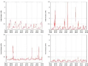
Figure 1 shows how this is not necessarily the case. Even on similar dwellings the customer behavior can be very diverse.
As some of the key technologies of Smart Grids are realized, the concerns regarding legacy infrastructure become more apparent. Increasing penetrations of micro-generation are challenging the usefulness of this assumption as excess domestic generation tips residential feeders into reverse power flows. While generation such as photovoltaic can be predicted to some degree of accuracy, there needs to be further work on modeling the loads that absorb them. Behavioral factors are identified in [2] that influence the load profile breaking energy demand into 2 root causes: behavioral determinants – habit driven, relatively flexible; and physical determinants –driven by environmental factors and building design. Behavioral drivers are the one which invoke most variability, [3] noted in an overview of advanced tariffs (e.g. real time pricing) that not all customers could be suited to these; demographics such as young families – no flexibility, constant temperature and the elderly who also require constant temperature. Then there are those who maintain a constant load already with the only losses stemming from dwelling disrepair/insulation shortcomings (cf. the‘physical determinants’ of [2]).
With consumer technology acquisition at its highest ever level, and expected to continue to grow, such profiles can only become invalid quicker thus reinforcing the case for data driven methodologies to be used. In this paper, an alternative representation of domestic load is considered, that of a composition of usage levels strata generated dynamically from
Enhanced Load Profiling for Residential
Network Customers
Bruce Stephen,
Member IEEE
, Antti Mutanen, Stuart Galloway, Graeme Burt
, Member IEEE
and
Pertti Järventausta,
Member IEEE
T
Figure 1: 30 minute resolution residential loads over a single week from similar dwellings.
probabilistic model allows a quantifiable comparison to be made between profiles generated by different dwellings and how these can change. This paper will present a framework for analyzing the consumption habits of domestic energy customers which will be illustrated through the application to actual half hourly metered properties.
II.RESIDENTIALLOADS
The absence of low voltage metering means that until recently very little knowledge exists on the low voltage customer’s true load profile. This section reviews some of the current practices and looks at how larger loads are dealt with on the medium voltage (MV) network.
A. Current Profiling Practice
The current practices tend to involve metering relatively small samples of households and then averaging over these. The following outlines examples from the UK and Finland.
1) United Kingdom
For the UK, it was decided in the mid-1990’s that to facilitate market operation, 8 load profiles would be used to represent the types of customers on the network. Of these profiles, Profile Class 1 [4] is the only one that represents the residential customer unconstrained by usage times. The form of the profile is 48 half hourly usage levels that correspond to the market settlement periods for every settlement day in a year. These are developed from recruited sample households with hi-resolution meters; homes in the samples for the 14 UK grid supply points are selected from rule based stratifications (high medium low) of annual consumption obtained from retail billing. Averages of the half hourly data are weighted by the proportions of the population at a given grid supply point in a given strata, yielding a load profile that takes the form of a 48×365 matrix.
2) Finland
Finnish electric utilities started to co-operate in load research in the 1980’s and in 1992 Finnish Electricity Association (FEA) published customer class load profiles for 46 different customer classes, 18 of which are for housing and the rest for agriculture, industry and services. The housing profiles are further divided by dwelling type, heating solution and major appliances. Each load profile contains expectation and standard deviation values for every hour of the year [5]. Although old, the FEA load profiles are still the only publicly available load profiles. The most prominent shortcoming of these profiles is their age; during the past 20 years electricity consumption has experienced significant changes, the amount of heat pumps and air-conditioners has multiplied, the use of entertainment electronics has increased and electricity consumption in recreational dwellings has changed [6]. Furthermore, in the future, the changes will be even bigger if plug-in hybrids, customer-specific distributed generation and demand response activities become popular. The load profiles
and errors caused by geographical generalization. The load profiles are created to model the average Finnish electricity consumption. They do not take into account the regional differences in electricity consumption, which originate from different climate conditions and socioeconomic factors. Consequently, the strategies used are error prone: the type of the customer is usually determined through a questionnaire when the electricity connection is contracted and then rarely updated. In reality, the customer type may change, for instance, because of a change in the heating solution, an addition of new devices, such as air conditioning or the change of customer activity e.g. from agriculture to pure housing.
B. Related Load Profiling on MV Network
In [7], Probabilistic Neural Networks (PNN) were used to assign consumers to load profiles–these are closely related to a Parzen Window and essentially smooth input data into a probability density function (PDF) of observations. 10 load profiles resulted but different cluster validity measures resulted in conflicting optimal number of clusters. An assortment of clustering techniques are used in [8] on 234 non-residential customers metered on the MV network at 15 minute intervals with the objective of grouping them into a small number of classes for tariff formulation. Reference [8] noted that theoretically robust means of choosing the number of clusters would be required as conflicts between cluster validity criteria could arise [7]. Techniques used include hierarchical clustering (with Euclidean distance), Self Organizing Maps, K-Means and Fuzzy K-K-Means. Dimensionality reduction of the 96-dimensional space into a more manageable subspace was also performedallowing the ‘informative’ hours/periods to be identified. ISODATA (Iterative Self Organizing Data Analysis Technique) was used in [9] to cluster industrial customers into load profile classes; outliers in training data were defined as customers with high intra-day variation and customers with high monthly variation were discarded.
Although load profiling on the MV network has received attention, the criteria associated with it are not the same; it was noted in [9] that large customers tend to have a small standard deviation in their load and hence produce a more accurate load profile lessening the need to encode variability in the profile representation thus emphasizing the need to encode variability in the smaller residential customer profiles as outlined in [10].
III. AMI/AMR STATUS
A number of countries are committed to upgrading their housing stock to Automated Meter Reading (AMR) systems or Smart Meters. In both the UK and Finland, large electricity customers are already metered on half hour or hourly basis but the state of domestic smart metering is different [11].
In Finland, full smart meter roll-out is currently underway and a significant number of meters have already been installed [11]. Legislation requires electricity distribution network operators to equip at least 80 % of their customers with hourly metering by the end of the year 2013. Daily meter reading, support to demand response, and outage registration are also
required [12]. One novel feature in Finnish AMR installations has been to integrate AMR system with control center applications of SCADA and DMS (Distribution Management System) in order to use AMR meters in real-time low-voltage network management and fault indication [13].
For the UK, AMR will provide advance data at a 30 minute resolution, most likely communicated at the end of a 24 hour period. Full scale roll-out is scheduled to begin in 2014 and finish in 2019 although some crucial parts of the program, such as details concerning national data and telecommunication services, are yet to be decided [14].
IV. RESIDENTIALPROFILINGREQUIREMENTS
Reference [15] identifies that ‘individual consumer behavior and their everyday practices accounts for a substantial proportion of household energy consumption’. In identical houses it was noted that this can vary by up to 300-400% as a result. The drivers for variability are multi-factorial: [16] identifies that different socio-economic types will contribute different amounts to energy demand using the Local Area Resource Access Model (LARA) – high levels of socioeconomic and geographical disaggregation were noted in the UK. Although the credit rating agency groups were noted, [16] uses UK OAC (Output Area Classification) to segment UK households into 7 groups with different socio-demographic characteristics with largely self explanatory labels e.g. ‘Blue Collar communities’, ‘City Living’, ‘Countryside’, ‘Prospering suburbs’. A ‘Culture based approachto behavior’is explored in [17] by identifying energy usage behaviors as a means of finding opportunities to invoke changes in behavior. In [17] the ’Energy Cultures’ framework was proposed to explain different causal facets of energy use which can be summarized as: Material Culture which is characterized by: insulation, heating devices and influenced by: Regulation, income, available technology; Cognitive norms which are characterized by: social aspiration, tradition, environmental concern and influenced by: Education, upbringing, demographics; Energy Practices which are characterized by: Number of rooms, Maintenance of technology and influenced by: Social Marketing, Energy Price Structure. As discussed, load profiles for the residential customer have been largely homogenous arrangements that were calendar based rather than behavior driven. With AMI/AMR/Smart Metering measurements providing extensive and detailed load and resulting variability, a representation is needed to capitalize on this and provide utility stakeholders with the information they require to increase reliability and efficiency. Regarding actual behavior, it is highly unlikely that all residential customers behave the same, so the representation must be able to accommodate a finite number of heterogeneous behaviors and do so in a compact manner thus enabling the representation to be utilized without unfeasibly large computing resources. For each heterogeneous behavior encountered, the traditional quantity of interest is the expected value of load; time of use is the other traditional concern so what is really required is a coupling of time of use with load magnitude. AMI in the UK and Finland provides data with half hour or one hour resolution allowing this quantity to be
represented as a discrete vector rather than a functional approximation. Where curve fitting or regressive approaches may not suffice is in the provision for capturing load variability–the confidence with which a given load’s expected value is expressed is also necessary. For forecasting purposes, which may arise in highly localized power systems, the relation between time of day loads can inform a short term forecast (weather related behavior change). Detection of anomalous behavior is another requirement that would provide indication of fault condition or, over longer terms, new classes of customer emerging (e.g. greatly reduced loads through adoption of storage or uptake of more efficient appliances). Additionally, the capture of changes in behavior should be allowed through the representation.
V.LOADMODELDESIGN
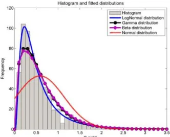
A. Load Probability Distributions
In load research, electric loads are often assumed to have a Gaussian distribution even though this is not the case. Previous studies [18, 19, 20] have tried to find the best probability distribution to model electric load behaviour. In these studies, beta, gamma, and log-normal distributions have been found to model electrical loads better than Gaussian distribution. Figure 2 shows that, when scored with Bayesian Information Criterion (BIC) [21], the log-normal distribution best describes UK residential loads out of several candidate probability distributions and is significantly better than the normal distribution. Also, by log-normalizing the data, it can be transformed to behave like a Gaussian distribution, which in turn enables the use of algorithms designed for the more
tractable Gaussian distribution.
B. Expressing Uncertainty through probabilistic models
The general form of models proposed in this paper is one of a non-stationary multivariate Gaussian distribution over 48 half hourly advance periods. In [20] it was noted that variability of even a single customer is such that an individual load pattern cannot be obtained – thus the importance of modeling the distribution rather than (just) the expected value. This section
Figure 2: Histogram and fitted distributions for half hour period 15:00-15:30 in January (weekdays only).
multimodality and dependence and in such a way that the representation maintains its compactness.
1) Mixture Models
A finite mixture model permits an arbitrary probability distribution to be approximated by a linear combination of weighted likelihoods drawn from a set of simple parametric distributions: M i i i
P
x
x
P
1;
θ
π
(1)If this were a Gaussian mixture model, then the components would be Gaussian parameterized as follows:
M i i i i
P
x
x
P
1 2,
;
µ
σ
π
(2)wherex is the observation variable,θ iis the parameter vector
for theithdistribution,π is the vector of mixing weights andM
is the number of distributions used to approximate the implied observation distribution.
2) Factor Analysis
As daily meter advances are represented as a 48 dimensional vector here, it is difficult to assess which times of use influence each other and how. Multivariate data can sometimes contain correlation between variables that are so strong, these can be amalgamated allowing only the most informative or uncorrelated variables to be represented in a space of reduced dimensionality. Two examples of models which can reduce the dimension of an observation space and thus discard uninformative variables and reveal dependency structure are Principal Component Analysis (PCA) [22] and Factor Analysis [23]. PCA is based around the eigenvectors that correspond to the eigenvalues of the covariance matrix of a multivariate observation. Factor Analysis assumes a linear mapping between such an observation spacexand its lower dimensional representationz:
u
z
x
µ
(3)Λ is the factor loading matrix that transforms observation x
into a lower dimensional representationz.µis the mean of the observation variable. Ψ is a diagonal covariance matrix attached to the zero mean distribution from which Gaussian noiseuis drawn.
,
0
~
N
u
(4)Factor Analysis does not impose the constraint of a common variance for all features and furthermore has a probabilistic model associated with it in the form of a Multivariate Gaussian
T
N
z
P
0
,
(5)Owing to the linear Gaussian semantics of the model the observation space is also assumed to be Gaussian
,
z
N
z
x
P
µ
(6)Λ is of particular use as interpretation of its rows/columns reveals the relations between variables in the observation space.
3) Mixtures of Factor Analyzers
For the situation where sub-populations exist in the observed data and multivariate dependency is non-homogeneous, the Factor Analysis model may be embedded in a mixture model [24]. M i i i i i
P
x
z
x
P
1,
;
µ
π
(7)Extending the mixture model to factor analysis, allows multiple sub-populations in a sub-space to be captured. The Mixture of Factor Analysers (MFA) model is particularly appealing to the load profiling application as it encodes not only the broad customer behaviors in the form of the model means but also expresses the variability over a day in a compact parameter set which also relates the advance times in terms of their variability.
C. Parameter Estimation and Model Order Selection
Beginning with a set of smart meter data there are two stages to go through before a model can be obtained: model selection and parameter estimation. Model selection decides on the cardinality of the model, the number of mixture components and the number of factors in the case of the Gaussian Mixture and MFA models previously discussed. Optimization techniques that estimate the parameters of statistical models from exemplar data are often based around Maximum Likelihood Estimation (MLE). Model order selection techniques often require parameters for a set of models to be learned then the optimal one chosen using some likelihood based measure such as BIC or Akaike Information Criterion (AIC):
M
x
P
N
X
AIC
N n n2
log
2
,
1θ
θ
(8)These select the most likely number of parameters M while penalizing overly complex models of a data population of size N. Model complexity can harm the generalization capabilities of a model by encoding too many specific eventualities in it.
While more complex parameter estimation techniques exist such as Monte Carlo based methods and Variational Inference, for illustrative purposes, the simpler Maximum Likelihood Estimate based formulation of the Expectation Maximization algorithm [25] can be used on both the mixture models and the Factor Analysers.
VI. LEARNEDRESIDENTIALLOADPROFILES
To illustrate the models proposed in this paper, load models are learned for a group of 32 residential customers. Since load behaviour is seasonal, separate load models are formed for each month. In the following examples, only January’s load models are shown.
A. Gaussian Mixture Load Model
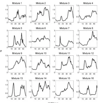
Using the January meter data for 32 residential properties, 50 Gaussian Mixture Models (GMM) were learned using maximum likelihood EM; from these 50 the optimal number of mixtures was selected using BIC, the results of which are shown in figure 3. Figure 3 demonstrates a pronounced minimum at 16 components but also reveals some important features of the data; the asymptotic behavior of the left-most extreme indicates that a single Gaussian distribution provides the poorest fit to the data which reinforces the need to provide for multimodal behaviour. Furthermore, a large number of behaviours does not adequately represent the behaviour of residential customers either– domestic loads would appear to have, as far as a Gaussian representation is concerned, a relatively small number of plausible forms, although as stated in the outset, not a single one.
One advantage of the Mixture model over say a Neural Network based clustering approach such as a self organizing map is that an element of determinism can be obtained through inspection of the parameters. Figure 4 shows the component means for the optimal parameterized GMM load model. This demonstrates the recurring load profile forms found in the 32 residential properties over the January period. One limitation of the Gaussian Mixture Model load profile is that owing to the high dimensionality of the data, it has difficulty expressing the dependence between advance times present in residential loads.
B. Mixture of Factor Analyzers Load Model
For an MFA mixture, an additional consideration is added to the model selection process in that one can trade off between mixtures (which accommodate various expected load profiles) and subspace dimensions (which capture the drivers of the correlation and variance structure).The MFA models offer even further insight into the nature of the load profiles discovered. Full covariance structure can be obtained for all mixture components regardless of the dimensionality of the data or the sparseness of the subpopulation that forms a mixture component. A covariance matrix can be reconstituted from the factor loading matrix as shown in equation (5), an
example of such a covariance matrix is shown in figure 5 as a heatmap representation: this shows how meter advances across the 48 daily intervals influence each other for a given load profile. Dark red areas are strong positive correlations i.e. when a given (row) advance increases, the corresponding (column) advance increases. Blue areas show negative correlation – increases in (row) advance size result in decreases in corresponding (column) advance. The 48 dimensional representation can pose difficulties in articulating in the relationships between advances due to the high dimensionality of the data [26]. The usefulness of covariance in load profiling is suggested by the example covariance matrix in Figure 5, which indicates dependencies between times of use, albeit as correlation. Advances around consecutive time periods (e.g. 10pm to 11:30pm) show a strong correlation reflecting late evening habits with little temporal variation and duration in the order of hours. Whereas the further apart the advance is the lower the correlation. Similar dependence structures are exhibited during the early hours of the morning as Figure 5 also demonstrates.
-1 -0.8 -0.6 -0.4 -0.2 0 0.2 0.4 0.6 0.8 1
Figure 5: Example covariance matrix from one component of a GMM. Note the very strong correlations for the advances in the early hours of the morning.
Figure 4: The 16 profile means found by the Gaussian Mixture.
Figure 3: Selection of the optimal number of customer profiles a GMM load model should represent.
This chapter shows how the above presented load models could be used in practice and compares their performance to existing load models.
A. Load Model Allocation
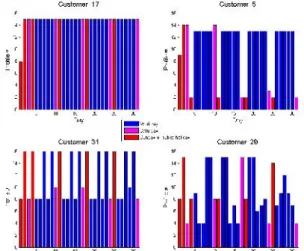
Before the learned load models can be used, they must be compiled into customer specific monthly load profiles. January’s load profile for all 32 customers can be compiled from the 16 previously learned day models, all we need to do is to find out which models best describe the customer’s behaviour on each day of the week. As an example, Figure 6 shows how the Gaussian Mixture load models are allocated for 4 different residential customers. Customer 17 shows remarkably consistent behavior, exhibiting the same profile for both weekday and weekend usage. Customer 29 switches between multiple profiles although does sometimes remain in the same one for more than one day. Customer 5 exhibits a near perfect separation in weekday/weekend electricity usage while Customer 31 switches between 3 profiles, always exhibiting the same energy usage characteristics on a Sunday. A single Gaussian distribution is not enough to describe a customer’sbehavior on each day of the week, so the final load model is constructed as a weighted average over all the mixtures in the model. This weighting is performed according to the occurrence counts of particular mixtures/profiles seen for a given customer during the period over which the training data was collected.
B. Comparison to Existing Load Models
In order to verify the accuracy of the proposed load modeling methodology, a comparison is made between the current British load modeling method (Standard Load Profile), GMM and MFA. February’s load forecasts are created using these methods and the forecasts are then compared to the real measured values. Since we have measurement data from only one year, the GMM and MFA model parameters are learned from January’s data while February’s measurements are reserved for verification. The selected Standard Load Profile (SLP) corresponds to the geographical location and type of the studied loads (domestic unrestricted customers). Both the
With 16 mixtures the AIC for MFA model is lowest with ten subspace dimensions. For comparison a MFA model with two dimensions is also built. The load forecasts were scaled to match the estimated energy consumption in February.
C. Load Flow Calculation
In practical applications, it is often important to estimate maximum (peak) or minimum (valley) loads. This is where the models of load variability are needed. When we know the load variability we can calculate peak or valley loads with different confidence levels. In Finnish network calculation, 95% confidence is typically used when calculating maximum line flows [27].
1) Simulation Network
The simulation network is based on a test network presented in [28]. Only the LV part of the test network is modeled in this study. The feeding MV network is modeled with a voltage source with 90 MVA short circuit power. The model incorporates a 500 kVA, 11 kV/433V ground mounted distribution transformer and four LV feeders each supplying 96 domestic customers. One LV feeder is modeled in detail and the other three are modeled as lumped loads, as shown in Figure 7. The LV feeder is 300 meters long, it comprises two segments of cable, 150 m of 185 mm2and 150 m of 95 mm2 cable. Single phase customer connections are distributed evenly along the feeder and are connected to the main feeder with 30 m long 35 mm2service cables. Load points of phase L1 are populated with real metered data.
2) Simulation Results
Statistical load flow was performed on the simulation network. Since there is no explicit method for summing log-normally distributed variables, the following simplification was made when summing loads during the load flow calculation: Expectation values and variances were calculated for the log-normally distributed loads, expectation values and variances were then summed and log-normal distribution parameters were recalculated as in [29]. Load flow was calculated for every half hour of February using three different load profiles: SLP, GMM and MFA based load profiles. With GMM and MFA models, 95% confidence level was used.
Figure 6: Demonstration of the daily variability of four residential customers
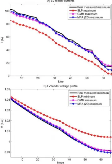
Maximum line currents and minimum node voltages were calculated and compared with the values calculated with real measured loads. Figure 8shows the estimated and “measured” maximum currents and minimum voltages on the phase L1 of the simulation network main feeder. The current and voltage values achieved with GMM and MFA models are very close to the real maximum and minimum values. Designing or operating the LV network based on Standard Load Profiles would be difficult since they don’t take the peak or valley load situations into account correctly. GMM and MFA models were superior compared to SLP model even though January’s load models were used to forecast February’s load. More accurate models could have been created if measurements from the
previous February had been available. Euclidean distance, Peak & Valley estimates and Peak & Valley estimates with 95% confidence, were calculated for both aggregated load estimates and their corresponding actual values; this comparison is shown in Table I. With GMM and MFA (2D) models, the smaller Euclidean distance demonstrates they track aggregated load better than the ones calculated with SLP. The MFA (10D) had a poor fit when evaluating performance with Euclidean distance which may be down to overfitting of the covariance matrices in the higher dimensional space.
VIII.CONCLUSIONS
This paper has presented several Linear Gaussian model based load profiling techniques that compactly capture multiple behaviors exhibited by residential customers who have traditionally been assumed to be homogenous. The combination of the modeling strategy and the smart meter advance data has permitted a representation that expresses not only load magnitudes at given times of day but also their variability and how these variabilities influence other times of use. The mixture model framework in which this is embedded allows multiple behaviors to be assumed with the statistically most likely one being used to categorize a given residential customer on a given day. In this way, dynamic customer behavior changes can be captured as they evolve with season or changes in routine. Such models have theoretical properties that permit ready use of sampling techniques that have been used to demonstrate gains in accuracy over existing load profile techniques. Such improvements are essential in the management of smaller and islanded power systems. Loss of performance in the MFA model may have stemmed from overfitting of the covariance matrices. In further work this could be prevented by considering a Bayesian formulation of MFA such as that proposed by [30], which has been shown to provide a more reliable estimate of optimal subspace dimensions. Attention should also now be turned to employing the computationally tractable Gaussian models in temporal and spatial models that could augment emerging state estimation tools [31] and models of regional energy density [32]. Both applications are increasingly important on LV networks as emerging services such as storage, distributed generation and demand response measures reach ever higher penetration levels.
TABLE I
ACCURACYMETRICS FORDIFFERENTLOADMODELS
Criteria SLP GMM MFA
(2D) MFA (10D) Euclidean distance 74.11 69.58 70.22 74.12 Peak estimate (real
23.1 kW) 19.32 18.62 18.69 18.26
Peak estimate with 95
% conf. interval - 22.69 23.20 22.73
Valley estimate (real
2.93 kW) 3.34 3.35 3.33 3.49
Valley estimate with
95 % conf. interval - 2.97 2.84 2.97
Figure 8: Load flow comparison between SLP, GMM and MFA models. A) Maximum currents on the LV main feeder (phase L1) B) Minimum voltages on the LV main feeder (phase L1)
[1] Partanen J., Juuti P., Lakervi E., A PC-based Network Information System for Power Distribution Companies and Consultants. Proceedings of the International Conference on High Technology in the Power Industry, Tainan, Taiwan, March 1991.
[2] Yao, R. & Steemers, K. A method of formulating energy load profile for domestic buildings in the UK. Energy and Buildings 37, pp. 663-671. Elsevier 2005.
[3] Alexander, B. Smart meters, real time pricing, and demand response programs: Implications for low income electric customers Oak Ridge National Lab, Technical Report, February 2007.
[4] Load Profiles and their use in Electricity Settlement. Available: http://www.elexon.co.uk/documents/participating_in_the_market/marke t_guidance_-_industry_helpdesk_faqs/load_profiles.pdf
[5] Seppälä, A. “Load research and load estimation in electricity distribution,” Ph.D. dissertation, Helsinki Univ. Technol., Espoo, Finland, 1996.
[6] Domestic electricity consumption 2006 (In Finnish). Adato Energia Ltd, Research report, 2.10.2008.
[7] Gerbec, D.; Gasperic, S.; Smon, I.; Gubina, F.; , "Allocation of the load profiles to consumers using probabilistic neural networks," Power Systems, IEEE Transactions on , vol.20, no.2, pp. 548- 555, May 2005. [8] Chicco, G., Napoli, R. & Piglione, F. “Comparisons Among Clustering
Techniques for Electricity Customer Classification”, IEEE Transactions on Power Systems, Vol. 21, No. 2, pp. 933-940, May 2006.
[9] Mutanen, A., Ruska, M., Repo, S. & Jarventausta, P., "Customer Classification and Load Profiling Method for Distribution Systems", IEEE Transactions on Power Delivery, Vol. 26, No. 3, pp.1755-1763, July 2011.
[10] Stephen, B. & Galloway, S. Domestic Load Characterization through Smart Meter Advance Stratification. IEEE Trans. Smart Grid, vol. 3, no. 3, pp. 1571-1572, September 2012.
[11] Annual Report on the Progress of Smart Metering 2009. European Smart Metering Alliance (ESMA) report, January 2010.
[12] REG 1.3.2009/66. Valtioneuvoston asetus sähköntoimitusten selvityksestä ja mittauksesta (Finnish council of state act on electricity settlement and metering).
[13] Järventausta P., Repo S., Rautiainen A. & Partanen J. Smart grid power system control in distributed generation environment. Elsevier Annual Reviews in Control 34 (2010) p. 277-286
[14] Smart Metering Implementation Programme: Response to Prospectus Consultation. Overview Document. Department of Energy & Climate Change (DECC), March 2011.
[15] Gram-Hanssen, K. “Standby consumption in households analysed with a practice theory approach”, Journal ofIndustrial Ecology 14:1, 2009. [16] Druckman, A. & Jackson, T. Household energy consumption in the UK:
A highly geographically and socio-economically disaggregated model Energy Policy 36, pp3177–3192, Elsevier 2008.
[17] Stephenson, J. Barton, B. Carrington, G. Gnoth, D. Lawson, R. & Thorsnes, P. Energy cultures: A framework for understanding energy behaviours. To appear, Energy Policy, Elsevier.
[18] Neimane V. Distribution Network Planning Based on Statistical Load Modeling Applying Genetic Algorithms and Monte-Carlo Simulations. IEEE Power Tech Conference, Porto, Portugal, 10-13 September. [19] Heunis S.W. & Herman R. A Probabilistic Model for Residential
Consumer Loads. IEEE Transactions on Power Systems, Vol. 17, No. 3, August 2002.
[20] Carpaneto E. & Chicco G. Probabilistic characterisation of the aggregated residential load patterns. IET Generation, Transmission & Distribution, 2007.
[21] Kass, R.E & Rafferty, A.E. Bayes Factors. Journal of the American Statistical Association Vol. 90, No. 430, Pages 773-795, American Statistical Association, June 1995.
[22] Jolliffe, I.T. Principal Components Analysis, Second Edition. Springer Series in Statistics, 2002.
[23] Everitt, B.S. Introduction to Latent Class Models. Chapman and Hill, London and New York. 1984.
[24] Ghahramani, Z. and Hinton, G.E. (1996) The EM Algorithm for Mixtures of Factor Analyzers. University of Toronto Technical Report CRG-TR-96-1, 8 pages (short note).
Statistical Society. Series B (Methodological), Vol.39, No.1, pp. 1-38, 1977.
[26] Tipping, M. E. and C. M. Bishop. Mixtures of Probabilistic Principal Component Analysers. Neural Computation 11(2), pp. 443–482, 1999. [27] Lakervi, E. & Holmes, E.J. Electricity distribution network design. 2nd
Edition. London 1995, Peter Peregrinus Ltd. 325 p.
[28] Ingram, S., Probert, S. & Jackson, K. The Impact of Small Scale Embedded Generation on the Operating Parameters of Distribution Networks. PB Power, October 2003, available at the DGCG website:http://webarchive.nationalarchives.gov.uk/20100919181607/htt p:/www.ensg.gov.uk/index.php?article=99
[29] Thomopoulos, N, & Johnson, A. (2003). Tables and characteristics of the standardized lognormal distribution. In Proceedings--Annual Meeting of the Decision Sciences Institute, pp 2379-2384.
[30] Ghahramani, Z. and Beal, M.J. (1999) Variational inference for Bayesian mixtures of factor analysers . In Neural Information Processing Systems 12.
[31] Singh, R., Pal, B. C. & Jabr, R. A. “Statistical Representation of Distribution System Loads Using Gaussian Mixture Model,” IEEE Transactions on Power Systems, vol. 25, no. 1, pp. 29-37, Feb. 2010. [32] Vale, Z., Morais, H. & Pereira, N. Energy Resources Scheduling in
Competitive Environment, Proceedings of CIRED 2011, Frankfurt, June 6th-9th 2011.
Dr Bruce Stephen (M ‘09) currently holds the post of Senior Research Fellow within the Institute for Energy and Environment at the University of Strathclyde. He received his B.Sc. from Glasgow University and M.Sc. and PhD degrees from the University of Strathclyde and is a Chartered Engineer. His research interests include Distributed Information Systems and Machine Learning applications in Power System Condition Monitoring and Asset Management.
Antti Mutanenwas born in Tampere, Finland, on June 10, 1982. He received his Master’s degree in electrical engineering from Tampere University of Technology in 2008. At present, he is a Researcher and a post-graduate student at the Department of Electrical Energy Engineering of Tampere University of Technology. His main research interests are load research and distribution network state estimation.
Dr Stuart Gallowayis a Senior Lecturer within the Institute for Energy and Environment. He obtained his MSc and PhD degrees in mathematics from the University of Edinburgh in 1994 and 1998 respectively. His research interests include power system optimization, numerical methods and simulation of novel electrical architectures.
Prof Graham Burt received his BEng in Electrical and Electronic Engineering from the University of Strathclyde in 1988. He received his PhD also from the University of Strathclyde in 1992. He is currently a Professor at the University of Strathclyde, and is Director of the University Technology Centre in electrical power systems, sponsored by Rolls Royce.
Prof Pertti Järventaustareceived his M.Sc. and Licentiate of Technology degrees in electrical engineering from Tampere University of Technology in 1990 and 1992 respectively. He received the Dr.Tech. degree in electrical engineering from Lappeenranta University of Technology in 1995. At present he is a Professor at the Department of Electrical Energy Engineering of Tampere University of Technology. The main interest focuses on the electricity distribution and electricity market.