DRAFT
Comparing Bayesian Models of Annotation
Silviu Paun1Bob Carpenter2Jon Chamberlain3 Dirk Hovy4Udo Kruschwitz3Massimo Poesio1
1School of Electronic Engineering and Computer Science, Queen Mary University of London 2Department of Statistics, Columbia University
3School of Computer Science and Electronic Engineering, University of Essex 4Department of Marketing, Bocconi University
Abstract
The analysis of crowdsourced annotations in NLP is concerned with identifying 1) gold standard labels, 2) annotator accuracies and biases, and 3) item difficulties and error patterns. Traditionally, majority voting was used for 1), and coefficients of agreement for 2) and 3). Lately, model-based analy-sis of corpus annotations have proven better at all three tasks. But there has been rel-atively little work comparing them on the same datasets. This paper aims to fill this gap by analyzing six models of annotation, covering different approaches to annotator ability, item difficulty, and parameter pool-ing (typool-ing) across annotators and items. We evaluate these models along four aspects: comparison to gold labels, predictive accu-racy for new annotations, annotator char-acterization, and item difficulty, using four datasets with varying degrees of noise in the form of random (spammy) annotators. We conclude with guidelines for model selec-tion, applicaselec-tion, and implementation.
1 Introduction
The standard methodology for analyzing crowd-sourced data in NLP is based on majority vot-ing (selectvot-ing the label chosen by the majority of coders) and inter-annotator coefficients of agree-ment, such as Cohen’s κ (Artstein and Poesio,
2008). However, aggregation by majority vote im-plicitly assumes equal expertise among the anno-tators. This assumption, though, has been repeat-edly shown to be false in annotation practice ( Poe-sio and Artstein, 2005; Passonneau and Carpen-ter, 2014;Plank et al., 2014b). Chance-adjusted coefficients of agreement also have many short-comings: e.g., agreements in mistake, overly large chance-agreement in datasets with skewed classes,
or no annotator bias correction (Feinstein and Ci-cchetti,1990;Passonneau and Carpenter,2014).
Research suggests that models of annotation can solve these problems of standard prac-tices when applied to crowdsourcing (Dawid and Skene, 1979; Smyth et al., 1995; Raykar et al.,
2010;Hovy et al.,2013;Passonneau and Carpen-ter, 2014). Such probabilistic approaches allow us to characterize the accuracy of the annotators and correct for their bias, as well as accounting for item-level effects. They have been shown to perform better than non-probabilistic alternatives based on heuristic analysis or adjudication (Quoc Viet Hung et al.,2013). But even though a large number of such models has been proposed ( Car-penter,2008;Whitehill et al.,2009;Raykar et al.,
2010;Hovy et al.,2013;Simpson et al.,2013; Pas-sonneau and Carpenter, 2014;Felt et al., 2015a;
Kamar et al., 2015; Moreno et al., 2015, inter alia), it is not immediately obvious to potential users how these models differ, or in fact, how they should be applied at all. To our knowledge, the literature comparing models of annotation is lim-ited; focused exclusively on synthetic data (Quoc Viet Hung et al., 2013) or using publicly avail-able implementations which constrain the exper-iments almost exclusively to binary annotations (Sheshadri and Lease,2013).
Contributions
• Our selection of six widely used models (Dawid and Skene,1979;Hovy et al.,2013;
Carpenter, 2008) covers models with vary-ing degrees of complexity: pooled models, which assume all annotators share the same ability; unpooled models, which model in-dividual annotator parameters; andpartially pooledmodels, which employ a hierarchical structure to let the level of pooling be dictated by the data.
DRAFT
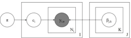
Figure 1: Plate diagram for multinomial model. Thehyperparameters are left out.
• We carry out the evaluation on four datasets with varying degrees of sparsity and annota-tor accuracy in both gold-standard dependent and independent settings.
• We use fully Bayesian posterior inference to quantify the uncertainty in parameter esti-mates.
• We provide guidelines for both model selec-tion and implementaselec-tion.
• We release all models evaluated here as Stan implementations atTBA.
Our findings indicate that models which in-clude annotator structure generally outperform other models, though unpooled models can over-fit. Several open-source implementations of each model type are available to users.
2 Bayesian Annotation Models
All Bayesian models of annotation we describe are generative: they provide a mechanism to generate parameters θ characterizing the process (annota-tor accuracies and biases, prevalence, etc.) from the priorp(θ), then generate the observed labelsy from the parameters according to the sampling dis-tributionp(y|θ). Bayesian inference allows us to condition on some observed datayto draw infer-ences about the parametersθ; this is done through the posterior,p(θ|y). The uncertainty in such in-ferences may then be used in applications such as jointly training classifiers (Smyth et al.,1995;
Raykar et al., 2010), comparing crowdsourcing systems (Lease and Kazai,2011), or characteriz-ing corpus accuracy (Passonneau and Carpenter,
2014).
This section describes the six models we eval-uate. These models are drawn from the litera-ture, but some had to be generalized from binary to multiclass annotations. The generalization nat-urally comes with parameterization changes, al-though these do not alter the fundamentals of the
Figure 2: Plate diagram of Dawid and Skene model.
models. (One aspect tied to the model parameter-ization is the choice of priors. The guideline we followed was to avoid injecting any class prefer-ences a priori and let the data uncover this infor-mation; see more in Section3)
2.1 A Pooled Model
Multinomial (MULTINOM) The simplest Bayesian model of annotation is the bino-mial model proposed in (Albert and Dodd,2004) and discussed in (Carpenter, 2008). This model pools all annotators (i.e., assumes they have the same ability; see Figure 1).1 The generative process is:
• For every classk∈ {1,2, ..., K}: – Draw class-level abilities
ζk∼Dirichlet(1K)2
• Draw class prevalenceπ∼Dirichlet(1K) • For every itemi∈ {1,2, ..., I}:
– Draw true classci ∼Categorical(π)
– For every positionn∈ {1,2, ..., Ni}:
∗ Draw annotation yi,n∼Categorical(ζci)
2.2 Unpooled Models
Dawid and Skene (D&S) The model proposed by Dawid and Skene (1979) is, to our knowledge, the first model-based approach to annotation pro-posed in the literature.3It has found wide
applica-tion (e.g., (Kim and Ghahramani, 2012;Simpson et al.,2013;Passonneau and Carpenter,2014)). It is an unpooled model, i.e., each annotator has their own response parameters (see Figure2), which are given fixed priors. Its generative process is:
1
Carpenter(2008) parameterizes ability in terms of speci-ficity and sensitivity. For multiclass annotations, we gener-alize to a full response matrix (Passonneau and Carpenter,
2014).
2
Notation:1Kis aK-dimensional vector of 1 values
3
Dawid and Skene fit maximum likelihood estimates us-ing expectation maximization (EM), but the model is easily extended to include fixed prior information for regularization, or hierarchical priors for fitting the prior jointly with the abil-ity parameters and automatically performing partial pooling.
DRAFT
• For every annotatorj∈ {1,2, ..., J}:– For every classk∈ {1,2, ..., K}: ∗ Draw class annotator abilities
βj,k ∼Dirichlet(1K)
• Draw class prevalenceπ∼Dirichlet(1K) • For every itemi∈ {1,2, ..., I}:
– Draw true classci ∼Categorical(π)
– For every positionn∈ {1,2, ..., Ni}:
∗ Draw annotation
yi,n∼Categorical(βjj[i,n],ci)
4
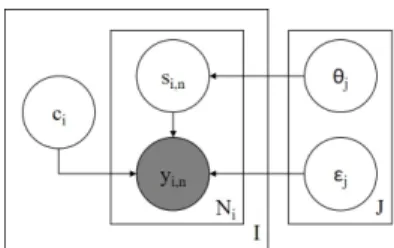
Multi-Annotator Competence Estimation (MACE) This model, introduced by Hovy et al.
(2013), takes into account the credibility of the annotators and their spamming preference and strategy5(see Figure3). This is another example of an unpooled model, and possibly the model most widely applied to linguistic data (e.g., (Plank et al.,2014a;Sabou et al.,2014;Habernal and Gurevych, 2016, inter alia)). Its generative process is:
• For every annotatorj∈ {1,2, ..., J}: – Draw spamming behavior
j ∼Dirichlet(10K)
– Draw credibilityθj ∼Beta(0.5,0.5)
• For every itemi∈ {1,2, ..., I}: – Draw true classci ∼U nif orm
– For every positionn∈ {1,2, ..., Ni}:
∗ Draw a spamming indicator si,n∼Bernoulli(1−θjj[i,n])
∗ Ifsi,n= 0then:
· yi,n=ci
∗ Else:
· yi,n∼Categorical(jj[i,n])
2.3 Partially-Pooled Models
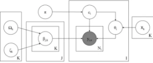
Hierarchical Dawid and Skene (HIERD&S) In this model, the fixed priors of Dawid and Skene are replaced with hierarchical priors representing the overall population of annotators (see Figure
4). This structure provides partial pooling, using information about the population to improve es-timates of individuals by regularizing toward the
4
Notation: jj[i,n] gives the index of the annotator who produced the n-th annotation on item i.
5I.e. propensity to produce labels with malicious intent.
Figure 3: Plate diagram for the MACE model.
Figure 4: Plate diagram for the hierarchical Dawid and Skene model.
population mean. This is particularly helpful with low count data as found in many crowdsourcing tasks (Gelman et al., 2013). The full generative process is as follows:6
• For every classk∈ {1,2, ..., K}: – Draw class ability means
ζk,k0 ∼Normal(0,1),∀k0 ∈ {1, ..., K}
– Draw class s.d.’s
Ωk,k0 ∼HalfNormal(0,1),∀k0
• For every annotatorj∈ {1,2, ..., J}: – For every classk∈ {1,2, ..., K}:
∗ Draw class annotator abilities βj,k,k0 ∼Normal(ζk,k0,Ωk,k0),∀k0
• Draw class prevalenceπ∼Dirichlet(1K) • For every itemi∈ {1,2, ..., I}:
– Draw true classci ∼Categorical(π)
– For every positionn∈ {1,2, ..., Ni}:
∗ Draw annotation yi,n ∼
Categorical(softmax(βjj[i,n],ci))
7
Item Difficulty (ITEMDIFF) We also test an ex-tension of the “Beta-Binomial by Item” model in (Carpenter,2008), which does not assume any an-notator structure; instead, the annotations of an item are made to depend on its intrinsic difficulty. The model further assumes that item difficulties
6
A two-class version of this model can be found in ( Car-penter,2008) under the name “Beta-Binomial by Annotator”.
7The argument of the softmax is aK-dimensional vector
of annotator abilities given the true class, i.e.,βjj[i,n],ci =
DRAFT
Figure 5: Plate diagram for item difficulty model.are instances of class-level hierarchical difficul-ties (see Figure5). This is another example of a partially-pooled model. Its generative process is presented below:
• For every classk∈ {1,2, ..., K}: – Draw class difficulty means:
ηk,k0 ∼Normal(0,1),∀k0 ∈ {1, ..., K}
– Draw class s.d.’s
Xk,k0 ∼HalfNormal(0,1),∀k0
• Draw class prevalenceπ∼Dirichlet(1K) • For every itemi∈ {1,2, ..., I}:
– Draw true classci ∼Categorical(π)
– Draw item difficulty θi,k ∼
Normal(ηci,k, Xci,k),∀k
– For every positionn∈ {1,2, ..., Ni}:
∗ Draw annotation:
yi,n∼Categorical(softmax(θi))
Logistic Random Effects (LOGRNDEFF) The last model is the Logistic Random Effects model (Carpenter,2008), which assumes the annotations depend on both annotator abilities and item dif-ficulties (see Figure6). Both annotator and item parameters are drawn from hierarchical priors for partial pooling. Its generative process is given be-low:
• For every classk∈ {1,2, ..., K}: – Draw class ability means
ζk,k0 ∼Normal(0,1),∀k0 ∈ {1, ..., K}
– Draw class ability s.d.’s Ωk,k0 ∼HalfNormal(0,1),∀k0
– Draw class difficulty s.d.’s Xk,k0 ∼HalfNormal(0,1),∀k0
• For every annotatorj∈ {1,2, ..., J}: – For every classk∈ {1,2, ..., K}:
∗ Draw class annotator abilities βj,k,k0 ∼Normal(ζk,k0,Ωk,k0),∀k0
Figure 6: Plate diagram for logistic random effects model.
• Draw class prevalenceπ∼Dirichlet(1K) • For every itemi∈ {1,2, ..., I}:
– Draw true classci ∼Categorical(π)
– Draw item difficulty: θi,k ∼Normal(0, Xci,k),∀k
– For every positionn∈ {1,2, ..., Ni}:
∗ Draw annotation yi,n ∼
Categorical(softmax(βjj[i,n],ci −
θi))
3 Implementation of the Models
We implemented all models in this paper in Stan (Carpenter et al., 2017), a tool for Bayesian In-ference based on Hamiltonian Monte Carlo. Al-though the non-hierarchical models we present can be fit with (penalized) maximum likelihood (Dawid and Skene, 1979; Passonneau and Car-penter, 2014),8 there are several advantages to a Bayesian approach. First and foremost, it pro-vides a mean for measuring predictive calibra-tion for forecasting future results. For a well-specified model that matches the generative pro-cess, Bayesian inference provides optimally cali-brated inferences (Bernardo and Smith,2001); for only roughly accurate models, calibration may be measured for model comparison (Gneiting et al.,
2007). Calibrated inference is critical for mak-ing optimal decisions, as well as for forecast-ing (Berger, 2013). A second major benefit of Bayesian inference is its flexibility in combining submodels in a computationally tractable manner.
8Hierarchical models are challenging to fit with classical
methods; the standard approach, maximum marginal likeli-hood, requires marginalizing the hierarchical parameters, fit-ting those with an optimizer, then plugging the hierarchical parameter estimates in and repeating the process on the co-efficients (Efron,2012). This marginalization requires either a custom approximation per model in terms of either quadra-ture or MCMC to compute the nested integral required for the marginal distribution that must be optimized first ( Mar-tins et al.,2013).
DRAFT
For example, predictors or features might beavail-able to allow the simple categorical prevalence model to be replaced with a multi-logistic regres-sion (Raykar et al., 2010), features of the anno-tators may be used to convert that to a regres-sion model, or semi-supervised training might be carried out by adding known gold-standard labels (Van Pelt and Sorokin, 2012). Each model can be implemented straightforwardly and fit exactly (up to some degree of arithmetic precision) using Markov chain Monte Carlo (MCMC) methods, al-lowing a wide range of models to be evaluated. This is largely because posteriors are much bet-ter behaved than point estimates for hierarchical models, which require custom solutions on a per-model basis for fitting with classical approaches (Rabe-Hesketh and Skrondal,2008). Both of these benefits make Bayesian inference much simpler and more useful than classical point estimates and standard errors.
Convergence is assessed in a standard fashion using the approach proposed byGelman and Ru-bin (1992): for each model we run four chains with diffuse initializations and verify that they converge to the same mean and variances (using the criterionR <ˆ 1.1).
Hierarchical priors, when jointly fit with the rest of the parameters, will be as strong and thus sup-port as much pooling as evidenced by the data. For fixed priors on simplexes (probability parameters that must be non-negative and sum to1.0), we use uniform distributions (i.e.,Dirichlet(1K)). For lo-cation and scale parameters, we use weakly infor-mative normal and half-normal priors that inform the scale of the results, but are not otherwise sen-sitive. As with all priors, they trade some bias for variance and stabilize inferences when there is not much data. The exception is MACE, for which we used the originally recommended priors, to con-form with the authors’ motivation.
All implementations will be made available to readers online atTBA.
4 Evaluation
The models of annotation discussed in this paper find their application in multiple tasks: to label items, characterize the annotators, or flag espe-cially difficult items. This section lays out the met-rics used in the evaluation of each of these tasks.
Dataset I N J K J/I I/J
WSD 177 1770 34 3 10 10 10 10 10 10 17 20 20 52 77 177 RTE 800 8000 164 2 10 10 10 10 10 10 20 20 20 49 20 800 TEMP 462 4620 76 2 10 10 10 10 10 10 10 10 16 61 50 462 PD 5892 43161 294 4 1 5 7 7 9 57 1 4 13 147 51 3395
Table 1: General statistics (Iitems,N observations,J
annotators, K classes) together with summary statis-tics for the number of annotators per item (J/I) and the number of items per annotator (I/J) (i.e., Min, 1st Quartile, Median, Mean, 3rd Quartile, and Max)
4.1 Datasets
We evaluate on a collection of datasets reflect-ing a variety of use-cases and conditions: binary vs. multi-class classification; small vs. large number of annotators; sparse vs. abundant num-ber of items per annotator / annotators per item; and varying degrees of annotator quality (statis-tics presented in Table 1). Three of the datasets – WSD, RTE and TEMP, created by Snow et al.
(2008) – are widely used in the literature on an-notation models (Hovy et al., 2013; Carpenter,
2008). In addition, we include thePhrase Detec-tives 1.0 (PD) corpus (Chamberlain et al., 2016) which differs in a number of key ways from the
Snow et al. (2008) datasets: it has a much larger number of items and annotations, greater sparsity, and a much greater likelihood of spamming due to its collection via a Game-With-A-Purpose. This dataset is also less artificial than the datasets in
Snow et al. (2008), which were created with the express purpose of testing crowd-sourcing. The data consists of anaphoric annotations, which we reduce to four general classes (DN/DO - discourse new/old, PR - property, and NR - non-referring). To ensure similarity with the Snow et al. (2008) datasets, we also limit the coders to one annotation per item (discarded data was mostly redundant an-notations). Furthermore, this corpus allows us to evaluate on meta-data not usually available in tra-ditional crowdsourcing platforms, namely infor-mation about confessed spammers and good, es-tablished players.
4.2 Comparison Against a Gold Standard The first model aspect we assess is how accu-rately they identify the correct (“true”) label of the items. The simplest way to do this is by
DRAFT
comparing the inferred labels against a goldstan-dard, using standard metrics such as Precision / Recall / F-measure, as done, e.g., for the evalua-tion of MACE in (Hovy et al., 2013). We check whether the reported differences are statistically significant, using bootstrapping (the shift method), a non-parametric two-sided test (Smucker et al.,
2007;Wilbur,1994). We use a significance thresh-old of 0.05 and further report whether the signifi-cance still holds after applying the Bonferroni cor-rection for type-1 errors.
This type of evaluation, however, presupposes that a gold standard can be obtained. This as-sumption has been questioned by studies show-ing the extent of disagreement on annotation even among experts (Poesio and Artstein, 2005; Pas-sonneau and Carpenter,2014;Plank et al.,2014b). This motivates exploring complementary evalua-tion methods.
4.3 Predictive Accuracy
In the statistical analysis literature, posterior pre-dictions are a standard assessment method for Bayesian models (Gelman et al.,2013). We mea-sure the predictive performance of each model us-ing thelog predictive density(lpd), i.e.,logp(˜y|y), in a BayesianK-fold cross-validation setting ( Pi-ironen and Vehtari,2017;Vehtari et al.,2017). The set-up is straightforward: we partition the data into Ksubsets, each subset formed by splitting the an-notations of each annotator into K random folds (we chooseK = 5). The splitting strategy ensures that models that cannot handle predictions for new annotators (i.e., unpooled models like D&S and MACE) are nevertheless included in the compari-son. Concretely, we compute
lpd= K X k=1 logp(˜yk|y(−k)) = K X k=1 log Z p(˜yk, θ|y(−k))dθ ≈ K X k=1 log 1 M M X m=1 p(˜yk|θ(k,m)) (1)
In (1),y(−k)andy˜krepresent the items from the
train and test data, for iterationkof the cross vali-dation, whileθ(k,m)is one draw from the posterior. 4.4 Annotators’ Characterization
A key property of most of these models is that they provide a characterization of coder ability.
In the D&S model, for instance, each annotator is modeled with a confusion matrix; Passonneau and Carpenter(2014) showed how different types of annotators (biased, spamming, adversarial) can be identified by examining this matrix. The same information is available in HIERD&S and LO-GRNDEFF, whereas MACE characterizes coders by their level of credibility and spamming prefer-ence. We discuss these parameters with the help of the meta-data provided by the PD corpus.
Some of the models (e.g., MULTINOM or ITEMDIFF) do not explicitly model annotators. However, an estimate of annotator accuracy can be derived post-inference for all the models. Con-cretely, we define the accuracy of an annotator as the proportion of their annotations that match the inferred item-classes. This follows the calculation of gold-annotator accuracy (Hovy et al., 2013), computed with respect to the gold standard. Simi-lar toHovy et al.(2013), we report the correlation between estimated and gold annotators’ accuracy.
4.5 Item Difficulty
Finally, the LOGRNDEFFmodel also provides an estimate which can be used to assess item diffi-culty. This parameter has an effect on the correct-ness of the annotators, i.e., there is a subtractive relationship between the ability of an annotator and the item-difficulty parameter. The ‘difficulty’ name is thus appropriate, although an examination of this parameter alone does not explicitly mark an item as difficult or easy. The ITEMDIFFmodel does not model annotators and only uses the diffi-culty parameter, but the name is slightly mislead-ing, since its probabilistic role changes in the ab-sence of the other parameter (i.e., it now shows the most likely annotation classes for an item). These observations motivate an independent measure of item difficulty, but there is no agreement on what such a measure could be.
One approach is to relate the difficulty of an item to the confidence a model has in assigning it a label. This way, the difficulty of the items is judged under the subjectivity of the models, which in turn, is influenced by their set of assumptions and data fitness. As in (Hovy et al., 2013), we measure the model’s confidence via entropy, to fil-ter out the items the models are least confident in (i.e. the more difficult ones) and report accuracy trends.
DRAFT
5 ResultsThis Section assesses the six models along dif-ferent dimensions. The results are compared with those obtained with a simple majority vote (MAJVOTE) baseline. We do not compare the results with non-probabilistic baselines as it has already been shown–see, e.g., Quoc Viet Hung et al.(2013)–that they underperform compared to a model of annotation.
We follow the evaluation tasks and metrics dis-cussed back in Section4 and briefly summarized next. A core task for which models of annota-tion are employed is to infer the correct interpreta-tions from a crowdsourced dataset of annotainterpreta-tions. This evaluation is conducted first and consists of a comparison against a gold standard. A problem with this assessment is caused by ambiguity, pre-vious studies indicating disagreement even among experts. Considering obtaining a true gold stan-dard is questionable, we further explore a comple-mentary evaluation, assessing the predictive per-formance of the models, a standard evaluation ap-proach from the literature on Bayesian models. Another core task models of annotation are used for is to characterize the accuracy of the annotators and their error patterns. This is the third objective of this evaluation. Finally, we conclude this Sec-tion assessing the ability of the models to correctly diagnose the items for which potentially incorrect labels have been inferred.
The PD data are too sparse to fit the models with item-level difficulties (i.e., ITEMDIFF and LOGRNDEFF). These models are therefore not present in the evaluations conducted on the PD corpus.
5.1 Comparison Against a Gold Standard A core task models of annotation are used for is to infer the correct interpretations from crowd-annotated datasets. This Section compares the in-ferred interpretations with a gold standard.
Tables2,3and4present the results.9 On WSD and TEMP datasets (see Table4), characterized by a small number of items and annotators (statistics in Table 1), the different model complexities re-sult in no gains, all the models performing equiv-alently. Statistically significant differences (0.05
9
The results for MAJVOTE, HIERD&S and LOGRND-EFFwe report match or slightly outperform those reported by (Carpenter,2008) on the RTE dataset. Similar for MACE, across WSD, RTE and TEMP datasets (Hovy et al.,2013).
Model Result Statistical Significance MULTINOM 0.89 D&S* HIERD&S*
LOGRNDEFF* MACE* D&S 0.92 ITEMDIFF* MAJVOTE
MULTINOM*
HIERD&S 0.93 ITEMDIFF* MAJVOTE* MULTINOM*
ITEMDIFF 0.89 LOGRNDEFF* MACE* D&S* HIERD&S* LOGRNDEFF 0.93 MAJVOTE* MULTINOM*
ITEMDIFF*
MACE 0.93 MAJVOTE* MULTINOM* ITEMDIFF*
MAJVOTE 0.90 D&S HIERD&S* LOGRNDEFF* MACE* Table 2: RTE dataset: results against the gold standard. Both micro (accuracy) and macro (P, R, F) scores are the same. * indicates that significance (0.05 threshold) holds after applying the Bonferroni correction.
threshold, plus Bonferroni correction for Type-1 errors; see Section 4.2 for details) are, how-ever, very much present in Tables2(RTE dataset) and 3 (PD dataset). Here the results are dom-inated by the unpooled (D&S and MACE) and partially-pooled models (LOGRNDEFF, and HI-ERD&S, except for PD, as discussed later in Sec-tion 6.1) which assume some form of annotator structure. Furthermore, modeling the full anno-tator response matrix leads in general to better re-sults (e.g., D&S vs. MACE on the PD dataset). Ignoring completely any annotator structure is rarely appropriate, such models failing to capture the different levels of expertise the coders have – see the poor performance of the unpooled MULTI-NOMmodel and of the partially-pooled ITEMDIFF model. Similarly, the MAJVOTEbaseline, implic-itly assumes equal expertise among coders, lead-ing to poor performance results.
5.2 Predictive Accuracy
Ambiguity causes disagreement even among ex-perts, affecting the reliability of existing gold stan-dards. This Section presents a complementary evaluation, i.e., predictive accuracy. In a simi-lar spirit to the results obtained in the compari-son against the gold standard, modeling the abil-ity of the annotators was also found essential for a good predictive performance (results presented in Table 5). However, in this type of evaluation,
DRAFT
Accuracy (micro) F-measure (macro)
Model Result Statistical Significance Result Statistical Significance
MULTINOM 0.87 D&S* HIERD&S* MACE* MAJVOTE 0.79 D&S* HIERD&S* MACE* MAJVOTE* D&S 0.94 HIERD&S* MACE* MAJVOTE* MULTINOM* 0.87 HIERD&S* MACE* MAJVOTE* MULTINOM* HIERD&S 0.89 MACE* MAJVOTE* MULTINOM* D&S* 0.82 MAJVOTE* MULTINOM* D&S*
MACE 0.93 MAJVOTE* MULTINOM* D&S* HIERD&S* 0.83 MAJVOTE* MULTINOM* D&S*
MAJVOTE 0.88 MULTINOMD&S* HIERD&S* MACE* 0.73 MULTINOM* D&S* HIERD&S* MACE*
Precision (macro) Recall (macro)
Model Result Statistical Significance Result Statistical Significance MULTINOM 0.73 D&S* HIERD&S* MACE* MAJVOTE* 0.85 HIERD&S* MAJVOTE* D&S 0.88 HIERD&S* MACE* MULTINOM* 0.87 HIERD&S MACE MAJVOTE* HIERD&S 0.76 MACE* MAJVOTE* MULTINOM* D&S* 0.89 MACE* MAJVOTE* MULTINOM* D&S MACE 0.83 MAJVOTEMULTINOM* D&S* HIERD&S* 0.84 MAJVOTE* D&S HIERD&S*
MAJVOTE 0.87 MULTINOM* HIERD&S* MACE 0.63 MULTINOM* D&S* HIERD&S* MACE*
Table 3: PD dataset: results against the gold standard. * indicates that significance holds after Bonferroni correc-tion.
Dataset Model Accµ PM RM FM
WSD ITEMDIFF 0.99 0.83 0.99 0.91 LOGRNDEFF Others 0.99 0.89 1.00 0.94 TEMP MAJVOTE 0.94 0.93 0.94 0.94 Others 0.94 0.94 0.94 0.94 Table 4: Results against the gold (µmicro; M macro)
the unpooled models can overfit, affecting their performance, e.g., a model of higher complex-ity like D&S, on a small dataset like WSD. The partially pooled models avoid overfitting through the hierarchical structure obtaining the best pre-dictive accuracy. Ignoring the annotator structure (ITEMDIFF and MULTINOM) leads to poor per-formance on all datasets except for WSD where this assumption is roughly apppropriate since all the annotators have a very high proficiency (above 95%).
5.3 Annotators’ Characterization
Another core task models of annotation are em-ployed for is to characterize the accuracy and bias of the annotators.
We first assess the correlation between the esti-mated and gold accuracy of the annotators. The re-sults, presented in Table6, follow the same pattern to those obtained in Section5.1: a better perfor-mance of the unpooled (D&S and MACE10) and partially-pooled models (LOGRNDEFF and HI -ERD&S, except for PD, as discussed later in Sec-tion6.1). The results are intuitive: a model that is
10
The results of our reimplementation match the published ones (Hovy et al.,2013)
Model WSD RTE TEMP PD*
MULTINOM -0.75 -5.93 -5.84 -4.67 D&S -1.19 -4.98 -2.61 -2.99 HIERD&S -0.63 -4.71 -2.62 -3.02 ITEMDIFF -0.75 -5.97 -5.84 -LOGRNDEFF -0.59 -4.79 -2.63 -MACE -0.70 -4.86 -2.65 -3.52
Table 5: The log predictive density results, normalized to a per-item rate (i.e.,lpd/I). Larger values indicate a better predictive performance. PD* is a subset of PD such that each annotator has a number of annotations at least as big as the number of folds.
accurate w.r.t. the gold standard should also obtain high correlation at annotator level.
The PD corpus comes also with a list of self-confessed spammers and one of good, established players (see Table 7 for a few details). Contin-uing with the correlation analysis, an inspection of the second-last column from Table 6 shows largely accurate results for the list of spammers. However, on the second category, i.e., the non-spammers (the last column), we see large differ-ences between models, following the same pattern with the previous correlation results. An inspec-tion of the spammers’ annotainspec-tions show an almost exclusive use of the DN (discourse new) class, which is highly prevalent in PD and easy for the models to infer; the non-spammers, on the other hand, make use of all the classes, making it more difficult to capture their behavior.11
11
In a typical coreference corpus over 60% of mentions are DN; thus always choosing DN results in a good accuracy level. The one-class preference is a common spamming be-havior (Hovy et al.,2013;Passonneau and Carpenter,2014).
DRAFT
Model WSD RTE TEMP PD S NS
MAJVOTE 0.90 0.78 0.91 0.77 0.98 0.65 line MULTINOM 0.90 0.84 0.93 0.75 0.97 0.84 D&S 0.90 0.89 0.92 0.88 1.00 0.99 HIERD&S 0.90 0.90 0.92 0.76 1.00 0.91 ITEMDIFF 0.80 0.84 0.93 - - -LOGRNDEFF 0.80 0.89 0.92 - - -MACE 0.90 0.90 0.92 0.86 1.00 0.98
Table 6: Correlation between gold and estimated accu-racy of annotators. The last two columns refer to the list of known spammers and non-spammers in PD
Type Size Gold accuracy quantiles Spammers 7 0.42 0.55 0.74
Non-spammers 19 0.59 0.89 0.94
Table 7: Statistics on player types. Reported quantiles are 2.5%, 50% and 97.5%.
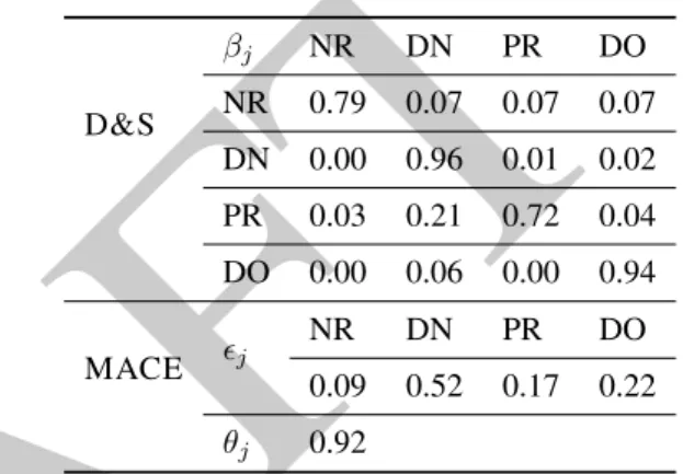
We further examine some useful parameter es-timates for each player type. We chose one spam-mer and one non-spamspam-mer and discuss the con-fusion matrix inferred by D&S, together with the credibility and spamming preference given by MACE. The two annotators were chosen to be representative for their type. The selection of the models was guided by their two different ap-proaches to capturing the behavior of the annota-tors.
Table8presents the estimates for the annotator selected from the list of spammers. Again, inspec-tion of the confusion matrix shows that, irrespec-tive of the true class, the spammer almost always produces the DN label. The MACE estimates are similar, allocating 0 credibility to this annotator, and full spamming preference for the DN class.
In Table9we show the estimates for the anno-tator chosen from the non-spammers list. Their response matrix indicates an overall good perfor-mance (see diagonal matrix), albeit with a con-fusion of PR (property) for DN (discourse new), which is not surprising given that indefinite NPs (e.g., a policeman) are the most common type of mention in both classes. MACE allocates large credibility to this annotator and shows a similar spamming preference for the DN class.
The discussion above, as well as the quantiles presented in Table 7, show that poor accuracy is not by itself a good indicator of spamming. A spammer like the one discussed in this section can get good performance by always choosing a class with high frequency in the gold standard. At
D&S βj NR DN PR DO NR 0.03 0.92 0.03 0.03 DN 0.00 1.00 0.00 0.00 PR 0.01 0.98 0.01 0.01 DO 0.00 1.00 0.00 0.00 MACE j NR DN PR DO 0.00 0.99 0.00 0.00 θj 0.00
Table 8: Spammer analysis example: D&S provides a confusion matrix; MACE shows the spamming prefer-ence and the credibility.
D&S βj NR DN PR DO NR 0.79 0.07 0.07 0.07 DN 0.00 0.96 0.01 0.02 PR 0.03 0.21 0.72 0.04 DO 0.00 0.06 0.00 0.94 MACE j NR DN PR DO 0.09 0.52 0.17 0.22 θj 0.92
Table 9: A non-spammer analysis example: D&S pro-vides a confusion matrix; MACE shows the spamming preference and the credibility.
the same time, a non-spammer may fail to recog-nize some true classes correctly, but be very good on others. Bayesian models of annotation allow capturing and exploiting these observations. For a model like D&S, such a spammer presents no harm, as their contribution towards any potential true class of the item is the same and therefore can-cels out.12
5.4 Filtering using Model Confidence
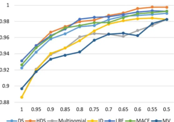
This Section assesses the ability of the models to correctly diagnose the items for which potentially incorrect labels have been inferred. Concretely, we identify the items the models are least confi-dent in (measured using the entropy of the poste-rior of the true class distribution) and present the accuracy trends as we vary the proportion of fil-tered out items.
Overall, the trends – Figures 7, 8 and 9 – in-dicate that filtering out the items with low
confi-12
This point was also made byPassonneau and Carpenter
DRAFT
Figure 7: Effect of filtering on RTE - accuracy (y-axis)vs. proportion of data with lowest entropy (x-axis)
Figure 8: TEMP dataset - accuracy (y-axis) vs. propor-tion of data with lowest entropy (x-axis)
dence improves the accuracy of all the models and across all datasets.13
6 Discussion
We found significant differences across a number of dimensions between both the annotation models and between the models and MAJVOTE.
6.1 Observations and Guidelines
The completely pooled model (MULTINOM) un-derperforms in almost all types of evaluation and all datasets. Its weakness derives from its core as-sumption: it is rarely appropriate in crowdsourc-ing to assume that all annotators have the same ability.
The unpooled models (D&S and MACE) as-sume each annotator has their own response pa-rameter. These models can capture the accuracy and bias of annotators, and perform well in all
13
The trends for MACE match the published ones. Also, we left out the analysis on the WSD dataset, as the models al-ready obtain 99% accuracy without any filtering (see Section
5.1).
Figure 9: PD dataset - accuracy (y-axis) vs. proportion of data with lowest entropy (x-axis)
evaluations against the gold standard. Lower per-formance is however obtained on posterior predic-tions: the higher complexity of unpooled models results in overfitting, which affects their predictive performance.
The partially pooled models (ITEMDIFF, HI-ERD&S and LOGRNDEFF) assume both individ-ual and hierarchical structure (capturing popula-tion behaviour). These models achieve the best of both worlds, letting the data determine the level of pooling that is required: they asymptote to the un-pooled models if there is a lot of variance among the individuals in the population, or to the fully pooled models when the variance is very low. This flexibility ensures good performance both in the evaluations against the gold standard and in terms of their predictive performance.
Across the different types of pooling, the mod-els which assume some form of annotator structure (D&S, MACE, LOGRNDEFF and HIERD&S) came out on top in all evaluations. The un-pooled models (D&S and MACE) register on par performance with the partially-pooled ones (LOGRNDEFFand HIERD&S, except for the PD dataset, as discussed later in this Section) in the evaluations against the gold, but as previously mentioned, can overfit, affecting their predic-tive performance. Ignoring any annotator struc-ture (the pooled MULTINOMmodel, the partially-pooled ITEMDIFFmodel, or the MAJVOTE base-line) leads generally to poor performance results.
The approach we took in this paper is domain independent, i.e., we did not assess and compare models that use features extracted from the data, even though it is known that when such features are available, they are likely to help (Raykar et al.,
DRAFT
is because a proper assessment of such modelswould also require a careful selection of the fea-tures and how to include them into a model of an-notation. A bad (i.e., misspecified in the statistical sense) domain model is going to hurt more than help as it will bias the other estimates. Providing guidelines for this feature-based analysis would have excessively expanded the scope of this pa-per. But feature-based models of annotation are extensions of the standard annotation-only mod-els; thus, this paper can serve as a foundation for the development of such models. A few examples of feature-based extensions of standard models of annotation are given in the Related Work section to guide readers who may want to try them out for their specific task/domain.
The domain-independent approach we took in this paper further implies there are no differences between applying these models to corpus anno-tation or other crowdsourcing tasks. This paper is focused on resource creation and does not pro-pose to investigate the performance of the mod-els in downstream tasks. However, previous work already employed such models of annotation for NLP (Plank et al., 2014a; Sabou et al., 2014;
Habernal and Gurevych, 2016), image labeling (Smyth et al.,1995;Kamar et al.,2015) or med-ical (Albert and Dodd,2004;Raykar et al.,2010) tasks.
While HIERD&S normally achieves the best performance in all evaluations on the Snow et al.
(2008) datasets, on the PD data it is outperformed by the unpooled models (MACE and D&S). To understand this discrepancy, it should be noted that the datasets fromSnow et al.(2008) were pro-duced using Amazon Mechanical Turk, by mainly highly skilled annotators; whereas the PD dataset was produced in a game-with-a-purpose setting, where most of the annotations were made by only a handful of coders of high quality, the rest be-ing produced by a large number of annotators with much lower abilities. These observations point to a single population of annotators in the for-mer datasets, and to two groups in the latter case. The reason why the unpooled models (MACE and D&S) outperform the partially-pooled HIERD&S model on the PD data is that this class of models assumes no population structure – hence there is no hierarchical influence; a multi-modal hierarchi-cal prior in HIERD&S might be better suited for the PD data. This further suggests that results
de-pend to some extent on the dataset specifics. This does not alter the general guidelines made in this study.
6.2 Technical Notes
Posterior curvature. In hierarchical models, a complicated posterior curvature increases the dif-ficulty of the sampling process affecting conver-gence. This may happen when the data is sparse or when there are large inter-group variances. One way to overcome this problem is to use a non-centered parameterization (Betancourt and Giro-lami, 2015). This approach separates the local parameters from their parents, easing the sam-pling process. This often improves the effective sample size and, ultimately, the convergence (i.e., lowerR). The non-centered parameterization of-ˆ fers an alternative but equivalent implementation of a model. We found this essential to ensure a ro-bust implementation of the partially-pooled mod-els.
Label Switching.The label switching problem that occurs in mixture models is due to the likelihood’s invariance under the permutation of the labels. This makes the models nonidentifiable. Conver-gence cannot be directly assessed, since the chains will not overlap anymore. We use a general solu-tion to this problem from Gelman et al. (2013): re-label the parameters, post-inference, based on a permutation that minimizes some loss function. For this survey, we used a small random sample of the gold data (e.g., five items per class) to find the permutation which maximizes model accuracy for every chain-fit. We then relabeled the parameters of each chain according to the chain-specific per-mutation before combining them for convergence assessment. This ensures model identifiability and gold alignment.
7 Related Work
Bayesian models of annotation share many char-acteristics with so called item-response and ideal-point models. A popular application of these mod-els is to analyze data associated with individuals and test items. A classic example is the Rasch model (Rasch,1993) which assumes that the prob-ability of a person being correct on a test item is based on a subtractive relationship between their ability and the difficulty of the item. The model takes a supervised approach to jointly estimating the ability of the individuals and the difficulty of
DRAFT
the test items based on the correctness of theirre-sponses. The models of annotation we discussed in this paper are completely unsupervised and in-fer, in addition to annotator ability and/or item dif-ficulty, the correct labels. More details on item-response models are given in (Skrondal and Rabe-Hesketh, 2004; Gelman and Hill, 2007). Item-response theory has also been recently applied to NLP applications (Lalor et al., 2016; Martınez-Plumed et al.,2016;Lalor et al.,2017).
The models considered so far take into account only the annotations. There is work, however, which further exploits the features that can accom-pany items. A popular example is the model intro-duced byRaykar et al.(2010), where the true class of an item is made to depend both on the annota-tions and on a logistic regression model which are jointly fit; essentially, the logistic regression re-places the simple categorical model of prevalence.
Felt et al.(2014,2015b) introduced similar mod-els which also modeled the predictors (features) and compared it to other approaches (Felt et al.,
2015a). Kamar et al. (2015) account for task-specific feature effects on the annotations.
In Section 6.2, we discussed the label switch-ing problem (Stephens, 2000) that many mod-els of annotation suffer from. Other solutions proposed in the literature include utilizing class-informative priors, imposing ordering constraints (obvious for univariate parameters; less so in mul-tivariate cases) (Gelman et al., 2013), or apply-ing different post-inference relabelapply-ing techniques (Felt et al.,2014).
8 Conclusions
This study aims to promote the use of Bayesian models of annotation by the NLP community. These models offer substantial advantages over both agreement statistics (used to judge coding standards), and over majority-voting aggregation to generate gold standards (even when used with heuristic censoring or adjudication). To provide assistance in this direction, we compare six exist-ing models of annotation with distinct prior and likelihood structures (e.g., pooled, unpooled, and partially pooled) and a diverse set of effects (anno-tator ability, item difficulty, or a subtractive rela-tionship between the two). We use various evalua-tion settings on four datasets, with different levels of sparsity and annotator accuracy, and report sig-nificant differences both among the models, and
between models and majority voting. As impor-tantly, we provide guidelines to both aid users in the selection of the models and to raise awareness of the technical aspects essential to their imple-mentation. We release all models evaluated here as Stan implementations atTBA.
Acknowledgments
Paun, Chamberlain and Poesio are supported by the DALI project, funded by ERC. Carpenter is partly supported by the U.S. National Science Foundation and the U.S. Office of Naval Research.
References
Paul S. Albert and Lori E. Dodd. 2004. A caution-ary note on the robustness of latent class models for estimating diagnostic error without a gold standard. Biometrics, 60(2):427–435.
Ron Artstein and Massimo Poesio. 2008. Inter-coder agreement for computational linguistics. Computational Linguistics, 34(4):555–596. James O. Berger. 2013. Statistical Decision
The-ory and Bayesian Analysis. Springer.
José M. Bernardo and Adrian F. M. Smith. 2001. Bayesian Theory. IOP Publishing.
Michael Betancourt and Mark Girolami. 2015. Hamiltonian Monte Carlo for hierarchical mod-els. Current trends in Bayesian methodology with applications, 79:30.
Bob Carpenter. 2008. Multilevel Bayesian models of categorical data annotation. Avail-able at http://lingpipe-blog.com/lingpipe-white-papers.
Bob Carpenter, Andrew Gelman, Matt Hoffman, Daniel Lee, Ben Goodrich, Michael Betancourt, Michael A. Brubaker, Jiqiang Guo, Peter Li, and Allen Riddell. 2017. Stan: A probabilistic programming language. Journal of Statistical Software, 76(1):1–32.
Jon Chamberlain, Massimo Poesio, and Udo Kr-uschwitz. 2016. Phrase Detectives corpus 1.0: Crowdsourced anaphoric coreference. In Pro-ceedings of the International Conference on Language Resources and Evaluation (LREC 2016), Portoroz, Slovenia.
DRAFT
Alexander Philip Dawid and Allan M. Skene.1979. Maximum likelihood estimation of ob-server error-rates using the EM algorithm. Ap-plied Statistics, 28(1):20–28.
Bradley Efron. 2012. Large-Scale Inference: Em-pirical Bayes Methods for Estimation, Testing, and Prediction, volume 1. Cambridge Univer-sity Press.
Alvan R. Feinstein and Domenic V. Cicchetti. 1990. High agreement but low kappa: I. The problems of two paradoxes. Journal of clinical epidemiology, 43(6):543–549.
Paul Felt, Kevin Black, Eric Ringger, Kevin Seppi, and Robbie Haertel. 2015a. Early gains matter: A case for preferring generative over discrimi-native crowdsourcing models. In Proceedings of the 2015 Conference of the North American Chapter of the Association for Computational Linguistics: Human Language Technologies. Paul Felt, Robbie Haertel, Eric K. Ringger,
and Kevin D. Seppi. 2014. MOMRESP: A Bayesian model for multi-annotator document labeling. In Proceedings of the International Conference on Language Resources and Eval-uation (LREC 2014), Reykjavik.
Paul Felt, Eric K. Ringger, Jordan Boyd-Graber, and Kevin Seppi. 2015b. Making the most of crowdsourced document annotations: Confused supervised LDA. In Proceedings of the Nine-teenth Conference on Computational Natural Language Learning, pages 194–203.
Andrew Gelman, John B. Carlin, Hal S. Stern, David B. Dunson, Aki Vehtari, and Donald B. Rubin. 2013. Bayesian Data Analysis, Third Edition. Chapman & Hall/CRC Texts in Sta-tistical Science. Taylor & Francis.
Andrew Gelman and Jennifer Hill. 2007.
Data Analysis Using Regression and Multi-level/Hierarchical Models. Analytical Methods for Social Research. Cambridge University Press.
Andrew Gelman and Donald B. Rubin. 1992. In-ference from iterative simulation using multiple sequences. Statistical science, 7:457–472. Tilmann Gneiting, Fadoua Balabdaoui, and
Adrian E. Raftery. 2007. Probabilistic fore-casts, calibration and sharpness. Journal of the
Royal Statistical Society: Series B (Statistical Methodology), 69(2):243–268.
Ivan Habernal and Iryna Gurevych. 2016. What makes a convincing argument? Empirical anal-ysis and detecting attributes of convincingness in Web argumentation. In Proceedings of the 2016 Conference on Empirical Methods in Nat-ural Language Processing, pages 1214–1223. Dirk Hovy, Taylor Berg-Kirkpatrick, Ashish
Vaswani, and Eduard Hovy. 2013. Learning whom to trust with MACE. In Proceedings of the 2013 Conference of the North Ameri-can Chapter of the Association for Computa-tional Linguistics: Human Language Technolo-gies, pages 1120–1130.
Ece Kamar, Ashish Kapoor, and Eric Horvitz. 2015. Identifying and accounting for task-dependent bias in crowdsourcing. In Third AAAI Conference on Human Computation and Crowdsourcing.
Hyun-Chul Kim and Zoubin Ghahramani. 2012. Bayesian classifier combination. In Proceed-ings of the Fifteenth International Conference on Artificial Intelligence and Statistics, pages 619–627, La Palma, Canary Islands.
John Lalor, Hao Wu, and hong yu. 2016. Building an evaluation scale using item response theory. InProceedings of the 2016 Conference on Em-pirical Methods in Natural Language Process-ing, pages 648–657. Association for Computa-tional Linguistics.
John P. Lalor, Hao Wu, and Hong Yu. 2017.
Improving machine learning ability with fine-tuning. CoRR, abs/1702.08563.
Matthew Lease and Gabriella Kazai. 2011. Overview of the TREC 2011 crowdsourcing track. In Proceedings of the text retrieval con-ference (TREC).
Fernando Martınez-Plumed, Ricardo B. C. Prudêncio, Adolfo Martınez-Usó, and José Hernández-Orallo. 2016. Making sense of item response theory in machine learning. In Proceedings of 22nd European Conference on Artificial Intelligence (ECAI), Frontiers in Artificial Intelligence and Applications, volume 285, pages 1140–1148.
DRAFT
Thiago G. Martins, Daniel Simpson, FinnLind-gren, and Håvard Rue. 2013. Bayesian comput-ing with INLA: New features. Computational Statistics & Data Analysis, 67:68–83.
Pablo G. Moreno, Antonio Artés-Rodríguez, Yee Whye Teh, and Fernando Perez-Cruz. 2015. Bayesian nonparametric crowdsourcing. Jour-nal of Machine Learning Research.
Rebecca J. Passonneau and Bob Carpenter. 2014. The benefits of a model of annotation. Transac-tions of the Association for Computational Lin-guistics, 2:311–326.
Juho Piironen and Aki Vehtari. 2017. Comparison of Bayesian predictive methods for model selec-tion. Statistics and Computing, 27(3):711–735. Barbara Plank, Dirk Hovy, Ryan McDonald, and Anders Søgaard. 2014a. Adapting taggers to Twitter with not-so-distant supervision. In Pro-ceedings of COLING 2014, the 25th Interna-tional Conference on ComputaInterna-tional Linguis-tics: Technical Papers, pages 1783–1792. Barbara Plank, Dirk Hovy, and Anders Sogaard.
2014b. Linguistically debatable or just plain wrong? In Proceedings of the 52nd Annual Meeting of the Association for Computational Linguistics (Volume 2: Short Papers).
Massimo Poesio and Ron Artstein. 2005. The re-liability of anaphoric annotation, reconsidered: Taking ambiguity into account. InProceedings of ACL Workshop on Frontiers in Corpus Anno-tation, pages 76–83.
Nguyen Quoc Viet Hung, Nguyen Thanh Tam, Lam Ngoc Tran, and Karl Aberer. 2013. An evaluation of aggregation techniques in crowd-sourcing. In Web Information Systems Engi-neering – WISE 2013, pages 1–15, Berlin, Hei-delberg. Springer Berlin HeiHei-delberg.
Sophia Rabe-Hesketh and Anders Skrondal. 2008. Generalized linear mixed-effects models. Lon-gitudinal data analysis, pages 79–106.
Georg Rasch. 1993. Probabilistic Models for Some Intelligence and Attainment Tests. ERIC. Vikas C. Raykar, Shipeng Yu, Linda H. Zhao, Gerardo Hermosillo Valadez, Charles Florin, Luca Bogoni, and Linda Moy. 2010. Learning
from crowds. Journal of Machine Learning Re-search, 11:1297–1322.
Marta Sabou, Kalina Bontcheva, Leon Derczyn-ski, and Arno Scharl. 2014. Corpus annotation through crowdsourcing: Towards best practice guidelines. InProceedings of the Ninth Interna-tional Conference on Language Resources and Evaluation (LREC-2014), pages 859–866. Aashish Sheshadri and Matthew Lease. 2013.
SQUARE: A benchmark for research on com-puting crowd consensus. InProceedings of the 1st AAAI Conference on Human Computation (HCOMP), pages 156–164.
Edwin Simpson, Stephen Roberts, Ioannis Pso-rakis, and Arfon Smith. 2013. Dynamic Bayesian Combination of Multiple Imperfect Classifiers. Springer Berlin Heidelberg, Berlin, Heidelberg.
Anders Skrondal and Sophia Rabe-Hesketh. 2004.
Generalized Latent Variable Modeling: Mul-tilevel, Longitudinal, and Structural Equation Models. Chapman & Hall/CRC Interdisci-plinary Statistics. Taylor & Francis.
Mark D. Smucker, James Allan, and Ben Carterette. 2007. A comparison of statisti-cal significance tests for information retrieval evaluation. In Proceedings of the Sixteenth ACM Conference on Conference on Information and Knowledge Management, CIKM ’07, pages 623–632, New York, NY, USA. ACM.
Padhraic Smyth, Usama M. Fayyad, Michael C. Burl, Pietro Perona, and Pierre Baldi. 1995. In-ferring ground truth from subjective labelling of Venus images. InAdvances in neural informa-tion processing systems, pages 1085–1092. Rion Snow, Brendan O’Connor, Daniel Jurafsky,
and Andrew Y. Ng. 2008. Cheap and fast - but is it good? Evaluating non-expert annotations for natural language tasks. In Proceedings of the Conference on Empirical Methods in Natu-ral Language Processing, pages 254–263. Matthew Stephens. 2000. Dealing with label
switching in mixture models. Journal of the Royal Statistical Society: Series B (Statistical Methodology), 62(4):795–809.
DRAFT
Chris Van Pelt and Alex Sorokin. 2012.De-signing a scalable crowdsourcing platform. In Proceedings of the 2012 ACM SIGMOD Inter-national Conference on Management of Data, pages 765–766. ACM.
Aki Vehtari, Andrew Gelman, and Jonah Gabry. 2017. Practical Bayesian model evaluation us-ing leave-one-out cross-validation and WAIC. Statistics and Computing, 27(5):1413–1432. Jacob Whitehill, Ting-fan Wu, Jacob Bergsma,
Javier R. Movellan, and Paul L. Ruvolo. 2009.
Whose vote should count more: Optimal inte-gration of labels from labelers of unknown ex-pertise. InAdvances in Neural Information Pro-cessing Systems 22, pages 2035–2043. Curran Associates, Inc.
W. John Wilbur. 1994. Non-parametric sig-nificance tests of retrieval performance com-parisons. Journal of Information Science, 20(4):270–284.