2016
Deep Learning for Decision Making and
Autonomous Complex Systems
Kin Gwn Lore
Iowa State UniversityFollow this and additional works at:
https://lib.dr.iastate.edu/etd
Part of the
Computer Sciences Commons, and the
Mechanical Engineering Commons
This Thesis is brought to you for free and open access by the Iowa State University Capstones, Theses and Dissertations at Iowa State University Digital Repository. It has been accepted for inclusion in Graduate Theses and Dissertations by an authorized administrator of Iowa State University Digital Repository. For more information, please [email protected].
Recommended Citation
Lore, Kin Gwn, "Deep Learning for Decision Making and Autonomous Complex Systems" (2016).Graduate Theses and Dissertations.
15965.
by
Kin Gwn Lore
A thesis submitted to the graduate faculty
in partial fulfillment of the requirements for the degree of MASTER OF SCIENCE
Major: Mechanical Engineering
Program of Study Committee: Soumik Sarkar, Major Professor
Baskar Ganapathysubramanian Chinmay Hegde
Iowa State University Ames, Iowa
2016
DEDICATION
I would like to dedicate this thesis to my major professor, Dr. Soumik Sarkar. Without his constant support and expert guidance, I would never have been able to complete this work with enthusiasm and become more well-versed in this field.
I would also like to dedicate this thesis to my family for their unconditional love and persistent support when completing this work.
TABLE OF CONTENTS
LIST OF TABLES viii
LIST OF FIGURES x
ACKNOWLEDGEMENTS xxi
ABSTRACT xxii
CHAPTER 1. INTRODUCTION 1
CHAPTER 2. DEEP LEARNING PRELIMINARIES 5
2.1 Architectures . . . 5
2.1.1 Restricted Boltzmann machines . . . 5
2.1.2 Deep neural networks . . . 9
2.1.3 Convolutional neural networks . . . 12
2.1.4 Stacked autoencoders . . . 16
2.2 Regularization . . . 18
2.2.1 Weight decay . . . 19
2.2.2 Early stopping . . . 19
PART I DEEP LEARNING FOR DECISION MAKING IN
MECHAN-ICAL SYSTEMS 23
CHAPTER 3. DATA-DRIVEN DEEP LEARNING MODELS FOR
EFFI-CIENT DESIGN OF MICROFLUIDIC FLOW PATTERNS 24
3.1 Motivation . . . 24
3.2 Problem setup . . . 27
3.3 Related approach: Genetic Algorithm . . . 28
3.4 Sequence prediction by Simultaneous Multiple Classification . . . 28
3.4.1 Training data generation using a metric on the output space . . . 30
3.4.2 Experiments and results . . . 32
3.5 Action sequence learning for causal shape transformation . . . 37
3.5.1 Proposed architectures . . . 39
3.5.2 Results and discussions . . . 44
3.6 Conclusions and Future Work . . . 46
CHAPTER 4. EARLY DETECTION OF COMBUSTION INSTABILITY US-ING HI-SPEED FLAME VIDEOS 49 4.1 Motivation . . . 49
4.2 Experimental Setup . . . 52
4.3 Deep learning and symbolic time series analysis: an integrated framework . . . . 55
4.4 Background on symbolic time series analysis (STSA) . . . 55
4.4.1 Generalized D-Markov machine [123] . . . 57
4.4.2 Construction of a D-Markov machine [94] . . . 58
4.4.3 Cross modeling for sensor fusion . . . 60
4.5 Early detection with DBN+STSA . . . 62
4.5.1 DBN feature visualization . . . 63
4.6 Early detection with CNN+STSA . . . 67
4.6.1 CNN training . . . 67
4.6.2 STSA-based instability measure with CNN . . . 68
4.6.3 Comparison of CNN+STSA with PCA+STSA . . . 70
4.7 Early detection with multimodal sensor fusion . . . 71
4.8 Early detection using deep convolutional selective autoencoders . . . 74
4.8.1 Convolutional Selective Autoencoder . . . 77
4.8.2 Instability measure . . . 78
4.8.3 Implementation . . . 78
4.8.4 Performance Evaluation . . . 80
4.9 Conclusion and Future Work . . . 85
PART II DEEP LEARNING FOR AUTONOMOUS COMPLEX SYS-TEMS 87 CHAPTER 5. DEEP VALUE OF INFORMATION ESTIMATORS FOR COL-LABORATIVE HUMAN-MACHINE INFORMATION GATH-ERING 88 5.1 Motivation . . . 88
5.2 Human-machine collaboration . . . 90
5.2.1 Problem setup . . . 90
5.2.2 Value of information (VOI) for soft/hard sensor scheduling . . . 93
5.3 Deep VOI estimators . . . 96
5.3.1 Design of framework . . . 97
5.4 Results and discussion . . . 99
5.4.1 Prediction accuracy . . . 99
5.4.2 Comparison with AMDP . . . 101
5.5 Semantic soft data scheduling . . . .104
CHAPTER 6. LLNET: A DEEP AUTOENCODER APPROACH TO
NAT-URAL LOW-LIGHT IMAGE ENHANCEMENT 109
6.1 Motivation . . . .109
6.2 Related work . . . 111
6.3 The Low-light Net (LLNet) . . . .112
6.3.1 Learning features from low-light images with LLNet . . . .112
6.3.2 Network parameters . . . .113
6.3.3 Training data generation . . . .114
6.3.4 Simulating darkness . . . .114
6.3.5 Image reconstruction . . . .116
6.4 Evaluation metrics and compared methods . . . .116
6.4.1 Performance metric . . . .116
6.4.2 Compared methods . . . .118
6.5 Results and discussion . . . .120
6.5.1 Algorithm adaptivity . . . .120
6.5.2 Enhancing artificially darkened images . . . .122
6.5.3 Enhancing darkened images in the presence of synthetic noise . . . .123
6.5.4 Application on natural low-light images . . . .126
6.5.5 Training with Gaussian vs. Poisson noise . . . 127
6.5.6 Denoising capability, image sharpness, and patch size . . . .129
6.5.7 Prior knowledge on input . . . .130
6.5.8 Features of low-light images . . . .132
6.5.9 Hyper-parameters, network architecture, and performance . . . .134
6.5.10 Color implementation . . . .134
CHAPTER 7. ROOT-CAUSE ANALYSIS FOR TIME-SERIES ANOMALIES VIA SPATIOTEMPORAL CAUSAL GRAPHICAL
MODEL-ING 138
7.1 Motivation . . . .138
7.2 Background and preliminaries . . . .140
7.2.1 Unsupervised anomaly detection with spatiotemporal graphical modeling .140 7.3 Methods . . . 141
7.3.1 Sequential state switching (S3) . . . 141
7.3.2 Artificial anomaly association (A3) . . . .144
7.4 Results and discussions . . . .145
7.4.1 Anomaly in pattern(s) . . . .145
7.4.2 Anomaly in node(s) . . . .147
7.4.3 Discussions . . . 151
7.5 Conclusions . . . 151
LIST OF TABLES
Table 3.1 Number of possible sequences,ns in an np-pillar sequence. . . 31
Table 3.2 PMR-based performance for DNN vs CNN. The appended number 4 is the number of pillars in the sequence. . . 33 Table 3.3 PMR-based performance for CNN with 7-pillar sequence that is trained with
randomly-generated training data vs. quasi-randomly generated training data. . . 33 Table 3.4 PMR and SSIM of regenerated flow shapes using different enhancement
methods. The numbers reported are in the format of [PMR/SSIM]. Bolded numbers correspond to the method with the highest PMR and SSIM. Asterisk (*) denotes our architecture presented in this paper. . . 47
Table 4.1 Description of operating conditions along with respective ground truth (stable or unstable) for hi-speed image data collection. 3s of greyscale
image sequence at3kHz is collected for each condition . . . 54
Table 6.1 PSNR and SSIM of outputs using different enhancement methods. ‘Bird’ means the non-dark and noiseless (i.e. original) image of Bird. ‘Bird-D’ indicates a darkened version of the same image. ‘Bird-D+GN18’ denotes a darkened Bird image with added Gaussian noise of σ = 18, whereas ‘Bird-D+GN25’ denotes darkened Bird image with added Gaussian noise of σ = 25. Bolded numbers corresponds to the method with the highest PSNR or SSIM. Asterisk (*) denotes our framework. . . 121
Table 6.2 Average PSNR and SSIM over 90 synthetic and 6 natural test images. Synthetic test images are randomly darkened withγ ∈[1,4]and Gaussian noise levels of σ ∈ [0,25]. Natural test images are taken under natural low-light conditions. Because gamma darkening is performed randomly for this set of images, we search for the optimalγ parameter that results in the highest SSIM (γ = 0.05 : 0.05 : 1) when applying gamma adjustment. Note that searching for the optimal parameter is infeasible in reality because no reference image is available. The number reported within the parentheses is the number of winning instances among 90 synthetic test images and 6 natural test images. Asterisk (*) denotes our framework. . . 121 Table 6.3 Average PSNR evaluated on the set of 90 test images enhanced with
trained model of different hyper-parameters and network architecture. The implemented model is marked by an asterisk (*), whereas the PSNR and SSIM for the best model are presented in bolded typeface. . . .133
Table 7.1 Root-cause analysis results inS3 method andA3 method with synthetic data.147 Table 7.2 Comparison of root-cause analysis results withS3 and VAR. . . 150
LIST OF FIGURES
Figure 2.1 Distinction between Boltzmann machines and restricted Boltzmann ma-chines. In RBMs, there are no interconnectivity between units within the same layer (i.e. visible-visible or hidden-hidden connections). . . 6 Figure 2.2 Simple and complex features for faces, cars, elephants, chairs, and other
objects. Figure courtesy of Lee et al. [74]. . . 10 Figure 2.3 Stacking restricted Boltzmann machines, RBMs (a) to form deep belief
networks, DBN (b). Adding a target layer on top will yield a deep neural network, DNN (c). . . 10 Figure 2.4 Structure of a CNN with multiple layers of convolutional and pooling
layers before the fully connected hidden layers. . . 13 Figure 2.5 The use of shared weights reduces memory footprints, preserves local
correlations, and reduces the number of learnable parameters to prevent overfitting. The colors of the sparse connections denote shared weights. . . 14 Figure 2.6 Convolving a filter (orange) over the input image (blue) to generate a
convolved feature map (green). For each output, the values of the filters are multiplied element-wise with the overlapping region in the input image. The products are summed up as one output element in the convolved feature. 14 Figure 2.7 The maxpooling scheme. The feature maps (blue) are divided into
non-overlapping partitions (shaded blues) where the maximum value is selected from each partition to form a new matrix (green). . . 15
Figure 2.8 Learning the identity function with an autoencoder (i-input, h-hidden unit, o-output). (a) The hidden layer is an identity function where the input can be fully reconstructed without loss. (b) Reduced number of hidden units captures the most important features to effectively reconstruct the input. (c) Sparsity constraints suppress activations of the hidden units to help extracting low-dimensional features from the input. . . 16 Figure 2.9 Training a single layer of denoising autoencoder. Input vectorxis corrupted
to obtain x˜. The objective is to learn the parameter θ that is able to reconstruct zfrom a compressed representation ofx˜ such that the error betweenz andx is minimized. The same parameter θis used in both the encoding and the decoding phase. . . 17 Figure 2.10 Stacking multiple autoencoders to form a deep architecture. The layers
are trained separately. . . 18 Figure 2.11 Effects of varying regularization parameter. Panel (a) shows a perfect
network being the ideal case. Panels (b) to (e) shows what happens when the regularization parameter λis increased. Panel (f) shows the situation whereλ=∞. . . 19 Figure 2.12 The early stopping algorithm prevents overfitting by evaluating losses on
both the training set and the validation set. . . 20
Figure 3.1 Pillar programming. Each pillar contributes to the deformation of the flow. The position-diameter pair of each pillar is assigned an index which will be used as class labels for classification. . . 27 Figure 3.2 CNN with the SMC problem formulation. . . 29 Figure 3.3 Uniform sampling vs. Quasi-random sampling. A set of 160 2-pillar
sequences are formed using uniform (left) and Sobol (right) sampling methods. The first 10 sampled sequences are shown in red, the next 50 sampled sequences in green, and the final 100 sampled sequences in blue. . 31
Figure 3.4 Eight example predictions (np = 4). The left side of each pair is the target
flow shape and the right side is the flow generated from the predicted pillar sequences. . . 32 Figure 3.5 Visualization of hidden layer activations in the DNN. . . 35 Figure 3.6 Visualization of CNN filters and feature maps of a test sample from
convolutional layers 1 and 2. . . 35 Figure 3.7 Comparison of pixel match rate and algorithm runtime for GA versus DL
methods (using CNN-SMC) to generate pillar sequences that has the best shape reconstruction closest to the target flow shape. Four examples are provided. . . 36 Figure 3.8 (a) Variation of theaverage PMR and training size ratio (ratio of training
samples to the number of all possible pillar sequences, on a logarithmic scale) with increasing number of pillars in a sequence. (b) Flow shapes generated from predicted pillar sequences. . . 37 Figure 3.9 The PPN addresses the question: ‘Given a pair of pre- and post-deformed
shape, what is the identity of the pillar causing the deformation?’ . . . 39 Figure 3.10 PPN-C treats the pre- and post-deformed shapes as separate channels. . . 40 Figure 3.11 The ITN addresses the question: ‘Given the final shape, what is the
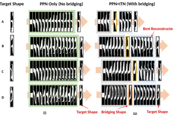
possible shape that lies in the middle of the nonlinear deformation pathway?’ 41 Figure 3.12 The integrated pipeline combining both PPN and ITN. . . 43 Figure 3.13 Four examples of sequence prediction using (i) PPN-only without bridging
and (ii) PPN+ITN with bridging. By predicting a bridging shape, the resulting predicted sequence is able to reconstruct flow shapes that are more similar to the target shape. Each frame shows the deformation on the flow shape with each additional predicted pillar added into the sequence. 45 Figure 3.14 Sample-wise (a) PMR and (b) SSIM comparison using CNN+SMC, PPN,
PPN-C, and PPN+ITN. 20 test target shapes are randomly generated with a 10-pillar sequence. . . 46
Figure 3.15 20 test shapes with reconstructed flow shapes generated from sequences predicted using different methods. Column A is the target shape, B for the reconstruction for CNN+SMC, C for PPN, D for PPN-C, and E for PPN+ITN. . . 48
Figure 4.1 (a) Schematic of the experimental setup. 1 - settling chamber, 2 - inlet duct, 3 - IOAM, 4 - test section, 5 - big extension duct, 6 - small extension ducts, 7 - pressure transducers,Xs - swirler location measured downstream from
settling chamber exit, Xp - transducer port location measured downstream
from settling chamber exit, Xi - fuel injection location measured upstream
from swirler exit, (b) Swirler assembly used in the combustor . . . 52 Figure 4.2 Top: greyscale images atRe= 7,971and full premixing for a fuel flow rate
of 0.495 g/s, bottom: greyscale images at Re= 15,942 and full premixing for a fuel flow rate of 0.495 g/s . . . 54 Figure 4.3 Framework for early detection of combustion instability from hi-speed
flame images via semantic feature extraction using deep belief network (DBN) followed by symbolic time series analysis (STSA) . . . 56 Figure 4.4 Variation of ×D-Markov entropy rate directed from time-series of DBN
hidden units (output of hi-speed video) to pressure time series as a func-tion of number of state splitting at a symbol size |Σ|= 3 for (a)stable combustion, (b) thermo-acoustically unstable combustion . . . 62 Figure 4.5 (d) Visualization of weights from the first layer and inputs that maximizes
the hidden unit activations for the (c) 1st layer, (b) 2nd layer, and (a) 3rd layer after pre-training and prior to supervised finetuning. . . 63 Figure 4.6 (d) Visualization of weights from 1st layer and inputs that maximizes the
hidden unit activations for the (c) 1st layer, (b) 2nd layer, and (a) 3rd layer after supervised finetuning. . . 64
Figure 4.7 0.2slong time series of l2 norms of (i) 10 largest variance components of
PCA performed on images at (a) stable and (b) unstable states and (ii) activation probabilities of last hidden layer after pre-training a DBN on images at (c) stable and (d) unstable states . . . 65 Figure 4.8 Variation of Euclidean distance between STSA features of image sequences
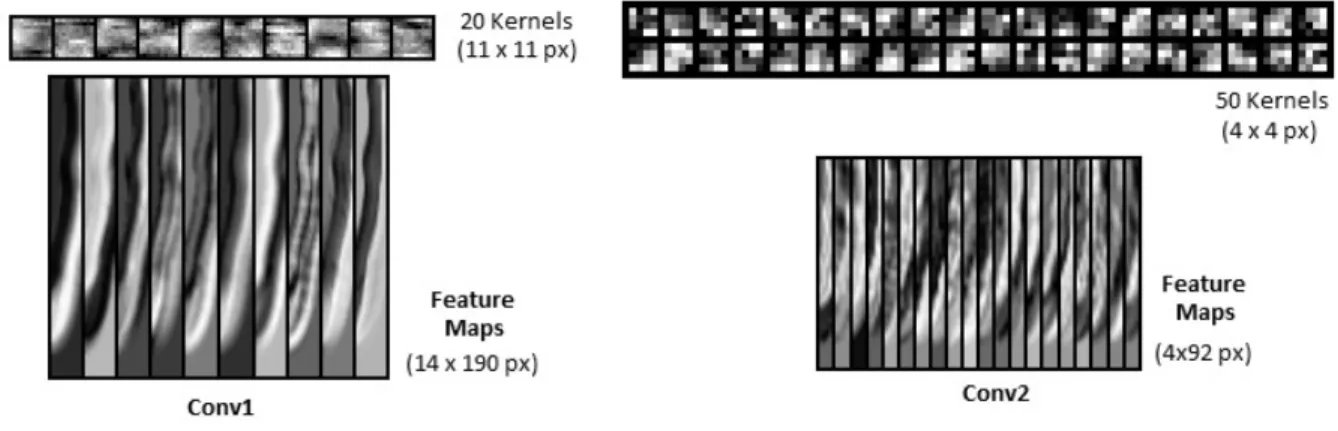
from stable and unstable combustion as a function of alphabet size for STSA 66 Figure 4.9 Filter visualization at convolutional layer (a) one and (b) two. (b) shows
fragmented representations of coherent structures that are visible in unsta-ble flame. (c) Feature maps of a staunsta-ble frame (top) and an unstaunsta-ble frame (bottom) after applying first convolutional layer filter. Red outline on the unstable flame visualization shows how the mushroom-shaped coherent structure is highlighted . . . 68 Figure 4.10 Variation of the proposed instability measure with time for the transition
video named 60050to35. Multiple regions on the measure curve denote
different combustion states such as stable, temporary intermittancy (a significant precursor to persistent instability) and unstable . They are corresponded to varied coherent structures (bounded by red box) that are detected by the ‘CNN+STSA’ framework. On the right, rmsvariation of the pressure is shown as it is one of the most commonly used instability measures. Progression of Prms can not detect the aforementioned precursors. 69
Figure 4.11 (a) Comparison of sudden change in instability measure when instablity sets in for different transition conditions which are 1. 50040to38, 2. 50040to30,
3. 40500to600, 4. 60050to35 and 5. 50700to800. The jump is larger for
‘CNN+STSA’ than ‘PCA+STSA’. (b) Variation of instability measure for both ‘CNN+STSA’ than ‘PCA+STSA’ at transition condition50700to800.
The measure arising from ‘CNN+STSA’ can detect the intermittancy precursor whereas it is mostly ignored by ‘PCA+STSA’. A frame with an intermittancy coherent structure in a red box is shown on the top. . . 70
Figure 4.12 Entropy rate as an instability measure at stable, relatively stable and unstable states for (a) D-Markov machine on pressure time series, (b)
×D-Markov machine directed from hi-speed video dominant-PCA-feature-aggregate time series to pressure time series, (c) ×D-Markov machine directed from hi-speed video bottleneck layer 5th hidden unit to pressure time series and (d) 10th hidden unit to pressure time series . . . 73 Figure 4.13 Grayscale images of gradual time-varying development of instability
struc-ture at two different parameter values . . . 75 Figure 4.14 Structure of the convolutional autoencoder with associated layer
parame-ters. The encoder portion extracts meaningful features from convolution and sub-sampling operations, while the decoder portion reconstructs the output into the original dimensions through deconvolution and upsampling. Unpooling is done with2×2upsampling by replicating the elements. Best viewed on screen, in color. . . 77 Figure 4.15 Schematics of implementation of trained network on transition test data . 79 Figure 4.16 Illustration of the pipeline’s ability to reproduce explicit labels. . . 80 Figure 4.17 Feature maps for (a) the third convolution layer, (b) the second pooling
layer, (c) the fourth convolution layer, (d) the unpooling layer and (e) the deconvolution layer. . . 81 Figure 4.18 Results of transition protocols for: a)60050to35, b)50040to30and c)50700to800
where purple arrows indicate expected results from stability and instability while the green arrows with different intensities indicate the strength of early instability presence in a supposedly stable region . . . 82 Figure 4.19 Adjacency labeling result of transition protocols for: a)60050to35, b)50040to30
and c) 50700to800 with three consecutive frames on a transition protocol
Figure 5.1 Sample truth model simulation of 2D target localization problem, showing locations of cameras 1-6 and associated fields of views, along with posterior distribution p(Xk|O1:k) (heat map) and true target location (magenta
x) for a random walk motion model p(Xk+1|Xk). Each sensor has 0.99
detection rate and false alarm rate of 1×10⁻⁴, 0.1504, 0.1585, 0.1992, 0.1510, and 0.1593, respectively. . . 92 Figure 5.2 Schematic of the CNN used for reward learning. . . 97 Figure 5.3 Four examples of belief map and VOI (discretized into bins) associated
with the action of switching into a particular sensor at different simulation time steps T. . . 99 Figure 5.4 Estimated VOI vs. True VOI for the first 40 out of 10,000 simulation
time steps. The figure also shows whether the sensor selected through rank-ordering the predicted VOI is the same as the sensor selected by ordering the true VOI, represented by green circles (matching) and red crosses (non-matching). . . 99 Figure 5.5 Degradation of selection accuracy with reduction of dataset sizes used to
train the CNN model. . . .100 Figure 5.6 Entropy of belief map over time. . . .102 Figure 5.7 Euclidean error between MAP estimate and target location over time. . .103 Figure 5.8 Error distribution between MAP estimate and target location. . . .103 Figure 5.9 The indoor search environment and associated semantic features for soft
observations. . . .105 Figure 5.10 The likelihood function that maps to the example observation, ‘Target is
near the dining table’. . . .106 Figure 5.11 Nine examples of CNN input showing the belief map, padding, and the
Figure 6.1 Architecture of the proposed framework: (a) An autoencoder module is comprised of multiple layers of hidden units, where the encoder is trained by unsupervised learning, the decoder weights are transposed from the encoder and subsequently fine-tuned by error back-propagation; (b) LLNet with a simultaneous contrast-enhancement and denoising module; (c) S-LLNet with sequential contrast-enhancement and denoising modules. The purpose of denoising is to remove noise artifacts often accompanying contrast enhancement. . . .113 Figure 6.2 Training the LLNet: Training images are synthetically darkened and added
with noise. These images are fed through LLNet where the reconstructed images are compared with the uncorrupted images to compute the error, which is then back-propagated to finetune and optimize the model weights and biases. . . 117 Figure 6.3 Original standard test images used to compute PSNR. . . .122 Figure 6.4 Comparison of methods of enhancing ‘Town’ when applied to (A) original
already-bright, (B) darkened, (C) darkened and noisy (σ= 18), and (D) darkened and noisy(σ= 25)images. Darkening is done withγ = 3. The numbers with units dB are PSNR, the numbers without are SSIM. Best viewed on screen. . . .123 Figure 6.5 Comparison of methods on randomly darkened/noise-added synthetic test
images of (A) Bird, (B) Girl, (C) Pepper, and (D) House. Darkening and noise addition are done using randomized values of γ ∈ [1,4] and
σ ∈[0,25]. The numbers with units dB are PSNR, the numbers without are SSIM. Best viewed on screen. . . .124
Figure 6.6 Comparison of methods of enhancing naturally dark images of (A) chalk-board, (B) computer, (C) objects, (D) chart, (E) cabinet, and (F) writings. Selected regions are enlarged to demonstrate the denoising and local con-trast enhancement capabilities of LLNet. HE (including HE+BM3D) results in overamplification of the light from the computer display whereas LLNet was able to avoid this issue. . . .125 Figure 6.7 The result of adding Gaussian noise and applying Poisson noise with
increasing photon count (normalized from 0 to 1 with a step size of 0.1). Although the noise levels between the two noise types look similar at higher photon count, the first three columns look very different. Best viewed on screen. . . .127 Figure 6.8 Natural low-light image enhancement results of LLNet trained with
Gaus-sian noise (LLNet-G) and Poisson noise (LLNet-P). ‘Gsn’ and ’Psn’ are abbreviations for Gaussian and Poisson respectively. Best viewed on screen.128 Figure 6.9 Relative patch size vs PSNR and SSIM. The picture with highest PSNR
has the highest denoising capability but least sharp. Picture with lowest
r has the least denoising capability but has the highest image sharpness. Picture with the highest SSIM balances between image sharpness and denoising capability. . . .130 Figure 6.10 Evaluation on US Air Force (USAF) resolution test chart. There exist
optimal relative patch sizes that result in the highest PSNR or SSIM after image enhancement (using LLNet). Note that the result enhanced with histogram equalization is shown to highlight the loss in detail of the natural dark image (where the main light is turned off) compared to the natural bright image. . . 131 Figure 6.11 Feature detectors can be visualized by plotting the weights connecting the
input to the hidden units in the first layer. These weights are selected randomly. . . .132
Figure 6.12 Random selection of weights from the first layer (feature detectors) and weights from the output layer (feature generators) for the integrated LLNet model trained with a patch size of 21×21. Patterns in the output weights are similar to patterns in the first hidden layer weights since tied weights are used. . . .132 Figure 6.13 Random selection of first layer weights from an integrated LLNet model
trained in batches of 1000 and 50, respectively. The superior model (i.e. batch size 50) learns features that appear more distinctive. . . .133 Figure 6.14 Enhancing natural low-light colored image with alternative methods. From
left to right: Natural dark, histogram equalization, gamma adjustment, histogram equalization with Color-BM3D (CBM3D), and LLNet. Best viewed on screen, in color (full resolution available when zoomed in). . . .137
Figure 7.1 Anomaly detection process. Spatiotemporal features are extracted from both nominal and anomalous data, with online STPN applied. Multiple sub-sequences of APs and RPs form input vectors to the RBM. Here, the RBM is only trained with nominal data, and the anomalous data is used as input to compute the free energy. Anomaly is detected by identifying its high energy state, which can be captured using the Kullback-Leibler Distance (KLD) metric. . . 141 Figure 7.2 Framing the problem as an artificial anomaly association (A3) problem.
(a) When training the model, the value of an element in both the input vector and its corresponding indicator label is randomly flipped to simulate anomaly. (b) When inferencing, a test input is fed into the DNN and a classification sub-problem is solved to obtain the indicator vector. Values of 0 in the output vector traces back to the exact patterns that are faulty. 145
Figure 7.3 Graphical models defined to simulate pattern(s) anomaly. Six graphs are defined and treated as nominal operation modes in complex systems. Pattern failure is simulated by breaking specific patterns in the model (not shown). . . .146 Figure 7.4 Anomalous conditions with fault node, causality is discovered by VAR
model. Compared with the nominal mode in Fig. 7.3(a), the fault node breaks most of the causality from and to this node. Causality is normalized by the maximal value among all of the patterns, and causality smaller than 0.03 is not shown. . . .148 Figure 7.5 Comparisons between sequential state switching (S3) method and vector
autoregressive (VAR) method using dataset3. The patterns represented with blocks are from the node in x-axis to the node in y-axis, and the discovered root causes are marked in black. . . .149
ACKNOWLEDGEMENTS
Continuing my graduate education has been a life-changing, unforgettable, and absolutely enjoyable journey of my life. I would like to use the opportunity to express my gratitude to everyone who has inspired me and helped me with various aspects in conducting the research.
First and foremost, I would like to express my sincerest gratitude and appreciation to Dr. Soumik Sarkar for his immeasurable amount of guidance, patience and support throughout this research and the writing of this thesis. His insights and words of encouragement are truly a blessing to me and have often inspired me to become an excellent, well-rounded practitioner of science. He is certainly a great mentor, a thoughtful friend, and a role model. I would also like to thank my committee members, Dr. Baskar Ganapathysubramanian and Dr. Chinmay Hegde, for providing insightful advice, efforts and contributions to this work.
I am especially grateful to my family for constantly offering emotional support while enrolled in the graduate program. I would also like to thank my friends in the laboratory and student office who have been best friends to share the joys of successful achievements and the griefs of having papers rejected for publication. Thank you all for being there for me during both good and bad times, and for making my time as a graduate student extremely delightful and memorable.
I would like to thank all of my collaborators. Without their invaluable opinions and expertise, I would never have produced tangible results from my research efforts. Along with my collaborators and co-authors, we sincerely acknowledge the extensive data collection performed by Vikram Ramanan and Dr. Satyanarayanan Chakravarthy at Indian Institute of Technology Madras (IITM), Chennai. The work has been supported in part by the National Science Foundation under Grant No. CNS-1464279, Iowa State Regents Innovation Funding, and Rockwell Collins Inc. We also gratefully acknowledge the support of NVIDIA Corporation with the donation of the GeForce GTX TITAN Black GPU used for this research.
ABSTRACT
Deep learning consists of various machine learning algorithms that aim to learn multiple levels of abstraction from data in a hierarchical manner. It is a tool to construct models using the data that mimics a real world process without an exceedingly tedious modelling of the actual process. We show that deep learning is a viable solution to decision making in mechanical engineering problems and complex physical systems.
In this work, we demonstrated the application of this data-driven method in the design of microfluidic devices to serve as a map between the user-defined cross-sectional shape of the flow and the corresponding arrangement of micropillars in the flow channel that contributed to the flow deformation. We also present how deep learning can be used in the early detection of combustion instability for prognostics and health monitoring of a combustion engine, such that appropriate measures can be taken to prevent detrimental effects as a result of unstable combustion.
One of the applications in complex systems concerns robotic path planning via the systematic learning of policies and associated rewards. In this context, a deep architecture is implemented to infer the expected value of information gained by performing an action based on the states of the environment. We also applied deep learning-based methods to enhance natural low-light images in the context of a surveillance framework and autonomous robots. Further, we looked at how machine learning methods can be used to perform root-cause analysis in cyber-physical systems subjected to a wide variety of operation anomalies. In all studies, the proposed frameworks have been shown to demonstrate promising feasibility and provided credible results for large-scale implementation in the industry.
CHAPTER 1. INTRODUCTION
Deep learning is a set of machine learning algorithms that aim to learn multiple levels of abstraction from data in a hierarchical manner. In other words, such algorithms operate on high-dimensional data that arrives in high volume, velocity, variety, veracity, and value. Oftentimes, solutions to various physical problems often involve constructing rigorous physical models to explain the observed phenomena in a highly detailed manner without neglecting the various sources of disturbance from the environment. Traditionally, engineers can only devise feasible solutions to a problem after laborious and time-consuming analysis, modeling, and data interpretation in producing reliable models. Due to the rapid advancement of technology, more and more problems need to be solved; there is a growing necessity to solve such problems as quickly and accurately as current technology allows. Unfortunately, it is an immensely tedious endeavour to construct new models all the time, which may potentially become too narrow in scope and limited in extensibility to other domains. Under these constraints, a scalable and fast modeling tool is desired.
Many domains such as engineering involve extensive collection and maintenance of large volumes of raw data for analysis and interpretation. As a data-driven approach, deep learning becomes an increasingly attractive option to create models based on these data generated by complex physical processes and simulation. A huge advantage is that the available data has already accounted for all disturbances and uncertainties coming from the natural environment. Further, deep learning algorithms perform feature extraction in an automated manner without feature hand-crafting; this powerful aspect of deep learning can be leveraged for high-level decision making. We show that in many cases, features extracted by deep learning algorithms from the data can provide sufficient insights to solve various problems without the overly-complex modeling of a physical phenomenon.
Deep learning is widely used in many problem areas ranging from object recognition [139, 40] and speech recognition [47, 29] to robotic perception [65] and human disease prediction [82]. In our study reported in Chapter3[84, 85], we demonstrate a novel application of deep learning in a mechanical design problem. Specifically, we learn from complex microfluidic flow patterns in order to solve inverse problems in fluid mechanics. A recent discovery enabled engineers to control the deformation of the cross-sectional shape of a flow by deliberately placing a sequence of pillars with varying positions and diameters [7]. This groundbreaking effort opens the door to rapid advancement in material science, manufacturing and biological applications. However, designing the sequences of pillars for user-defined deformations requires laborious and time-consuming design iterations. The problem is also exacerbated when the nonlinear design space has as large as1015 possibilities of flow shapes for a 10-pillar sequence. We demonstrate that hierarchical feature extraction techniques lead to scalable design tools by learning semantic representations from a relatively small number of flow patterns examples. In this study, we proposed various architectures including deep neural networks (DNN), convolutional neural networks (CNN), and stacked autoencoders (SAE) and compared their performance to the current state-of-the-art genetic algorithm (GA). Results show that the deep learning based design process is shown to expedite the current state-of-the-art design approach by over 600 times with competitive performance.
We also worked with our collaborators (as co-authors) to design a framework in the context of prognostics and health monitoring with relevant results published in [122, 121, 6, 117] and shown in Chapter4. Specifically, we propose a neural-symbolic framework for analyzing a large volume of sequential high-speed images of flames in engines for the early detection of combustion instability that is extremely critical for engine health. The proposed hierarchical approach involves extracting low-dimensional semantic features from images using deep CNNs followed by capturing the temporal evolution of the extracted features using symbolic time series analysis (STSA). The semantic nature of the CNN features enables expert-guided data exploration that can lead to better understanding of the underlying physics. Extensive experimental data have been collected in a swirl-stabilized dump combustor at various operating conditions for validation.
Another application concerning the robotic path planning via effective human-machine collaboration is published as [86] and presented in Chapter5. An effective collaboration may improve a large number of learning and planning strategies to gather information through the fusion ofhard data originated from machine sensors andsoft data originated from human sensors. However, gathering the most informative data from the human counterparts without task overloading remains a technical challenge. In this context, Value of Information (VOI) is a crucial decision-theoretic metric for scheduling interaction with human sensors. Naturally, deep learning becomes an attractive method to be used as a VOI estimation framework to schedule collaborative human-machine sensing with the advantage of computationally efficient online inference and minimal policy hand-tuning. We propose that supervised feature extraction from the image representation of the belief space using CNNs can be associated with soft data query choices to compute the corresponding VOI for human interaction in a reliable manner. The performance of the proposed framework is compared with a feature-based scheduling policy modeled using the partially-observed Markov decision process (POMDP). The practical feasibility of the method is demonstrated on a realistic mobile robotic search problem with language-based semantic human sensor inputs.
Mobile robots are also frequently deployed as part of a surveillance and monitoring framework as well as in tactical reconnaissance. In this context, gathering visual information from a dynamic environment and accurately processing such data are essential to making informed decisions and ensuring the success of a mission. Cameras are often required to capture images or videos in a lowly illuminated environment. Therefore, it is desirable to perform brightness and contrast enhancement and simultaneously reduce noise content from the image frames in an on-board real-time manner. In Chapter6, we tackle the problem of natural low-light image enhancement using deep autoencoders where the proposed algorithm is able to adaptively enhance image contrast without saturation effects while reducing image noise as a result of contrast enhancement. We show that a variant of the stacked-sparse denoising autoencoder can learn from synthetically darkened and noise-added training examples to enhance images taken from natural low-light images. The chapter presents the published article from [83] with additional results.
Aside from human-machine interaction systems, cyber-physical systems play a huge role in many engineering processes. It is not uncommon for modern distributed cyber-physical systems to encounter anomalies in any cases. When neglected, these systems are vulnerable to catastrophic fault propagation due to the strong connectivity between different sub-systems. Analyzing the root cause may become highly intractable due to the complex mechanism of fault propagation with a large variety of operating modes. In Chapter 7(published as [80]), we present a data-driven framework using machine learning methods to circumvent these issues in root-cause analysis. We propose the technique of sequential state switching (S3) using restricted Boltzmann machines (RBM) and artificial anomaly association (A3) using DNN for root-cause analysis in an unsupervised and semi-supervised manner respectively. Synthetic data from cases with failed patterns and anomalous node are simulated to validate the proposed approaches, then compared with the performance of vector autoregressive (VAR) model-based root-cause analysis. We show that these machine learning based methods result in satisfactory performance in terms of accuracy and capability in handling multiple modes.
CHAPTER 2. DEEP LEARNING PRELIMINARIES
In this chapter, a brief background on key deep learning concepts as well as the various architectures used in our studies is presented.
2.1 Architectures
There are various deep architectures available at our disposal to solve a variety of different problems. Here, we will present the theory behind restricted Boltzmann machines, deep belief networks, deep neural networks, convolutional neural networks, and stacked autoencoders. All of these architectures are core components to deep learning with fundamentally different mechanics. They may be mixed-and-matched into interesting combinations depending on the type of the task at hand.
2.1.1 Restricted Boltzmann machines
Restricted Boltzmann machine (RBM) is a generative stochastic artificial neural network that learns features in an unsupervised manner based on a probabilistic model [51]. It is first invented under the name Harmonium by Paul Smolensky in 1986 [131]. Later, it was popularized by Geoffrey Hinton and his collaborators during the rise of machine learning when the group developed fast learning algorithms to effectively train RBMs. RBMs have been repeatedly used in a diverse area of applications as a means to reduce data dimension [144], solving classification problems [71, 72], feature learning [19], collaborative filtering [114], and topic modeling [152, 52, 135]. The success of RBMs largely owes to the fact that the extracted features being nonlinear in nature. Therefore, it often generates good results when used in conjunction with a linear classifier such as support vector machines (SVM) or a perceptron. Internally, an RBM attempts to maximize the likelihood of the data using a particular graphical
model, typically employing the learning algorithm viastochastic maximum likelihood.Using this method, it is capable of capturing persistent regularities from the data and learning a probability distribution over the set of the provided inputs. However, to effectively train the RBM model we require a sufficiently large dataset.
Visible Units Hidden Units
(a) Boltzmann Machine (b) Restricted Boltzmann Machine
Figure 2.1: Distinction between Boltzmann machines and restricted Boltzmann machines. In RBMs, there are no interconnectivity between units within the same layer (i.e. visible-visible or hidden-hidden connections).
Restricted Boltzmann machines are actually a variant of Boltzmann machines [1]. In a Boltzmann machine, nodes, orneurons in the same group are connected in addition to nodes from the other group (Fig.2.1). Typically, two groups are present in a Boltzmann machines–they are often referred to as the visible or hidden units respectively. However, the interconnectedness of all the neurons within and between groups may complicate modeling. Hence, a restricted
version of the Boltzmann machine is used with a constraint that the neurons must form a bipartite graph where there are no connections within a group. This restriction make learning easier, as the hidden units become conditionally independent given the visible states [13]. RBMs are also the building blocks to deep neural networks (DNN), where they can be stacked to increase the modeling capacity. The architecture will be discussed in Section 2.1.2.
Architecture description for an RBM:A standard form of RBM is binary valued where the hidden and visible units take values of either 0 or 1. Between the visible and hidden layers there is a weight matrix W = (wi,j) of sizem×ndenoting the connection between visible unit
units and hidden units respectively. With these notations in mind, the energy function E(v, h)
of an RBM can be expressed as:
E(v, h) =−X i aivi− X j bjhj− X i X j viwi,jhj
or more compactly, in vector form:
E(v, h) =−aTv−bTh−vTW h
The joint probability distribution over hidden and visible units can now be defined in terms of the energy function as:
P(v, h) = e −E(v,h)
Z
where Z is a normalizing factor called the partition function with the following form, defined as the sum ofe−E(v,h) over all possible configurations:
Z =X
v,h
e−E(v,h)
In other words, the normalizing factorZ ensures that the probability distribution sums to 1. The marginal probability of the visible vector is the sum over all possible hidden layer configurations with: P(v) = 1 Z X h e−E(v,h)
With no connections between the hidden and visible layers, activations of the hidden units are mutually independent given the activations of the visible units. Likewise, the visible unit activations are also mutually independent given the activations of the hidden units. Therefore, if we have m visible units andn hidden units, then we can write the conditional probabilities as:
P(v|h) = m Y i=1 P(vi|h), P(h|v) = n Y j=1 P(hj|v)
Thus, the activation probabilities for each neuron is given by:
P(hj = 1|v) =σ bj+ m X i=1 wi,jvi ! , P(vi = 1|h) =σ ai+ n X j=1 wi,jhj
whereσ is a sigmoidal function, such as a logistic sigmoid σ1:
σ1(x) =
1 1 +e−x
or the hyperbolic tangent function σ2 which rescales the logistic sigmoid function to have an
output range between -1 and 1:
σ2(x) = tanh(x) =
ex−e−x ex+e−x
Training an RBM: Restricted Boltzmann machines can be trained with the objective to maximize the product of probabilities assigned to a training set denoted by matrix V. The objective is to obtain a weight matrixW such that:
W∗=argmaxW Y
v∈V
P(v)
It will be simpler to express the equation as a sum rather than product. Equivalently, the algorithm aims to maximize the expected log probability of V with:
W∗=argmaxWE " X v∈V logP(v) #
Maximizing the expected log probability is equivalent to minimizing it. We thus define the loss function as the negative of the log probability, and aim to minimize it via the gradient descent algorithm using the update equations:
W :=W −α∂logp(v) ∂W a:=a−α∂logp(v) ∂a b:=b−α∂logp(v) ∂b
whereα denotes the learning rate of the algorithm. The derivatives are expressed as follows [13]:
∂logp(v) ∂Wij =−Ev[p(hi|v)·vj] +vj(i)σ(Wi·v(i)) +ai ∂logp(v) ∂ai =−Ev[p(hi|v)] +σ(Wi·v(i)) ∂logp(v) ∂bj =−Ev[p(vj|h)·vj] +v(ji)
2.1.2 Deep neural networks
Deep neural networks (DNN) are obtained by stacking multiple layers or RBMs together. The more hidden layers are added to the network, the higher its nonlinear modeling capacity. Deep neural networks are also known as artificial neural networks (ANN), which are inspired by the observations and biological models proposed by Harvard neurophysiologists David H. Hubel and Torsten Wiesel. Hubel and Wiesel inserted a microelectrode into the primary visual cortex of an anesthetized cat and projected light and dark patterns on a screen in front of the cat. They found that some neurons of the cat fired rapidly depending on the angle of the presented lines. These neurons are referred to assimple cells. Further, they found that some other neurons (called complex cells) respond to the movement directions of the lines, which represents more complex stimuli. From these observations, they showed how the visual system builds complex representations from simple stimuli which established the fundamental concepts of deep learning [53, 148, 149, 112].
In deep neural networks, each layer of the neurons trains on different sets of features using the outputs from the previous layer. The deeper we advance into the network, the higher the complexity of the features that the netwwork can recognize. For example, in the application of face recognition, the first layer of the network usually learns primitives such as simple edges and curves. As we move on to the intermediate layers, the hidden layers begin learning a combination of these primitives, such as the eyes, the mouth, the ears, and the nose. The deepest layers are capable of combining the parts and begin recognizing faces (see Fig. 2.2). This concept widely known as the hierarchy of features, that is, a hierarchy of features with increasing complexity and abstraction. Therefore, deep networks are suited for handling a large of amount of very high-dimensional data sets.
Architecture description for an DNNs: In deep neural networks, the outputs of one layer become the input to the another layer. For the first layer, we have:
x2=f(W1v+b1)
wherex2 denotes the output of the first layer and the input to the second layer,W is the weight
Simple
Complex
Figure 2.2: Simple and complex features for faces, cars, elephants, chairs, and other objects. Figure courtesy of Lee et al. [74].
(a) Restricted Boltzmann Machine
(b) Stacking an RBM on top of another RBM
(c) Adding a target layer
RBM RBM Visible layer Hidden layer 1 Hidden layer 2 Target layer
Figure 2.3: Stacking restricted Boltzmann machines, RBMs (a) to form deep belief networks, DBN (b). Adding a target layer on top will yield a deep neural network, DNN (c).
modern deep nets prefer using the Rectified Linear Unit (ReLU) as the activation function over sigmoidal functions (e.g. the logistic sigmoid and tanh) due to the function being nonsaturating and provides good gradients conducive to training [97]. For all subsequent layers, we can generalize the equation to:
xk+1=f(Wkxk+bk), k >= 2
Supervised training of DNNs: Weight updates can be done via the stochastic gradient descent algorithm using the following equation, similar to one used to train RBMs:
θ:=θ−α∂C ∂θ
In this equation, θdenotes the model parameters which include the weights and biases of the layer. C is the cost function, or the loss function depending on the type of the problem we are attempting to solve. If the problem we are interested in is a classification problem, the zero-one loss and the negative log-likelihood loss are suitable candidates for the loss function. When using zero-one loss, a classifier is trained to minimize the number of errors on unseen examples. The loss can be written as:
`0,1=
|D| X
i=0
Ig(x(i))6=y(i)
where D is the training set, g is the prediction function with g : RD → {0, ..., L}, I is the indicator function, and Lis the number of output nodes corresponding to the class labels. The indicator function is defined as:
Ix= 1 if x is True 0 otherwise and that: g(x) =argmaxkP(Y =k|x, θ)
What this means is that the predicted class is the class with the highest probability given the input. However, the zero-one loss is not a differentiable loss function. This may pose some issues when optimizing the model due to the problem with a non-smooth gradient where the computations may become overly expensive. Hence, we focus our attention on maximizing the log-likelihood of the classifier given the labels in a training set:
L(θ,D) = |D| X
i=0
logP(Y =y(i)|x(i), θ)
Maximizing the log-likelihood is equal to minimizing the negative log-likelihood. Therefore, the loss function is rewritten as:
NLL(θ,D) =− |D| X
i=0
logP(Y =y(i)|x(i), θ)
If one wishes to perform regression using a deep neural network, then a natural choice of the loss function is to minimize the`2-norm (for example) of the difference between the output of
the neural network yˆwith the target vector y:
Unsupervised greedy layer-wise pretraining of deep belief networks (DBN):When training a DNN, the model parameters are initialized randomly as means of symmetry breaking. However, randomly initialized weights may slow training and cause the model to converge to bad local optima. To combat this, the deep neural network can be pretrained in a greedy layer-wise manner without labeled data (hence it is a deep belief network rather than deep neural network), using the same algorithm used to train an RBM [36]. After the first layer is trained, we keep the weights and biases of the first layer constant. The transformed input from the layer is utilized to train the next layer. This process is repeated for the desired number of layers in the network with each iteration propagating either the samples or mean activations to higher levels. As training continues, the product of probabilities assigned to the input is maximized. Once all the layers are trained, the pre-trained model parameters are finetuned via supervised backpropagation.
2.1.3 Convolutional neural networks
Deep neural networks have demonstrated success in image recognition. However, they quickly suffers from the curse of dimensionality if the input data dimensions is large. For example, recognizing a32×32-pixel color (RGB) image from the CIFAR-10 dataset will result in the first layer having width×height×channels= 32×32×3 = 3,072weights in the first layer. Practically, most inputs in image recognition applications are much larger than32×32 pixels. For example, a 512×512-pixel RGB image will now result in 512×512×3 = 786,432weights. Hence, we observe that the framework becomes intractable with larger input dimensions.
There are a few drawbacks to using DNNs in such cases. Firstly, the large number of fully connected layers will result in an excessively huge model when used in conjunction with a multi-layered deep network. Inferencing will take a longer time due to the increased computational complexity. Secondly, fully connected layers do not take into account the spatial structure of the image data and do not consider the local correlation of the features in the context of a two-dimensional image. Consequently, it places equal weighting on pixels that are close and far apart. Full connectivity clearly wastes valuable computational resources. Furthermore, the large number of parameters will be difficult to train and makes the network prone to overfitting.
Feature Maps
(Edge detectors) Fully connected
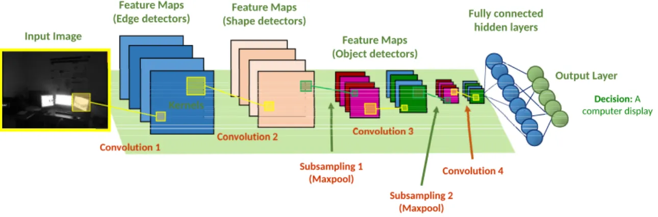
hidden layers Convolution 1 Convolution 2 Subsampling 1 (Maxpool) Convolution 3 Convolution 4 Subsampling 2 (Maxpool) Output Layer Input Image Kernels Decision: A computer display Feature Maps (Shape detectors) Feature Maps (Object detectors)
Figure 2.4: Structure of a CNN with multiple layers of convolutional and pooling layers before the fully connected hidden layers.
Convolutional neural networks (CNN) [65] are fundamentally different than regular DNNs in terms of architecture. It mitigates the issues posed by DNNs by exploiting the local 2D-correlations in input images, thus making it a very attractive model for working with image data. Unlike DNNs, neurons within a layer of CNN (called a receptive field) are only connected to a small region of the previous layer, as shown in Fig. 2.5. This ensures that the learned filters generates the strongest response according to a spatially local input pattern. By stacking multiple layers of filters together, the modeling capacity of the architecture becomes increasingly non-linear and captures more global features. Hence, at deeper levels the model can assemble lower-level features to form higher-level features.
The convolutional layer: Convolution is a sliding function (a filter) applied to the 2D input matrix. The convolutional layer is the most important building block of a CNN and consists of filters (or kernels) that can be learned. These filters have small receptive fields to extract local structures and uses shared weights (Fig. 2.5). With a set of different filters, the filters may specialize in detecting different features–the activations of different filters will depend on the specific type of feature at some spatial location in the input image. As the filters are convolved over the input, feature maps are generated (as illustrated in Fig.2.6). Stacking the feature maps along the depth dimension gives rise to the full output volume of the convolutional layer.
m m-1 Sparse connectivity Full connectivity m m-1
Figure 2.5: The use of shared weights reduces memory footprints, preserves local correlations, and reduces the number of learnable parameters to prevent overfitting. The colors of the sparse connections denote shared weights.
1 1 1 0 0 1 1 0 0 0 0 0 0 1 1 0 x1 x1 x0 x1 x0 x1 x0 x1 x0 3 1 1 1 0 0 1 1 0 0 0 0 0 0 1 1 0 x1 x1 x0 x1 x0 x1 x0 x1 x0 3 3 1 1 1 0 0 1 1 0 0 0 0 0 0 1 1 0 x1 x1 x0 x1 x0 x1 x0 x1 x0 3 3 1 1 1 1 0 0 1 1 0 0 0 0 0 0 1 1 0 x1 x1 x0 x1 x0 x1 x0 x1 x0 3 3 1 3
Figure 2.6: Convolving a filter (orange) over the input image (blue) to generate a convolved feature map (green). For each output, the values of the filters are multiplied element-wise with the overlapping region in the input image. The products are summed up as one output element in the convolved feature.
There are three most prominent hyperparameters that control the size of the output volume. With a deep layer, many neurons connect to a particular region in the input volume. The neurons will learn to activate different depending on the features in the input. For instance, neurons in the same layer may become active in the presence of edges in different orientations and lie in the same feature hierarchy. Large convolution strides will result in a smaller feature map due to less overlapping receptive fields, whereas small convolution strides (such as1×1) convolution will result in strongly overlapping receptive fields and, subsequently, larger feature maps. In all cases, the dimensions will be reduced depending on the size of the convolution strides. However, it is sometimes desirable to preserve the original spatial dimensions of the input volume. To achieve this, the borders of the input volume can be padded with zeros (termed as zero-padding) such that after the convolution operation, the reduced spatial dimensions are compensated to maintain original dimensions.
The pooling layer: Pooling is a form of nonlinear downsampling. Common practices employ the maxpooling scheme, where a2×2 matrix for example is downsampled into a1×1
1 3 1 0 2 5 0 0 1 2 2 3 0 1 1 0 5 1 3 2
Figure 2.7: The maxpooling scheme. The feature maps (blue) are divided into non-overlapping partitions (shaded blues) where the maximum value is selected from each partition to form a new matrix (green).
functions exist too; one may downsample by averaging the values or even computing the`2-norm.
Pooling is useful because it removes redundancies and helps reducing the dimensions of the data. The intuition is that once a feature is detected, the exact location of the feature may not be as important as the approximate location relative to other features. Doing so also reduces the number of learnable parameters to combat overfitting as well as reducing computation time. Note that using pooling layers is up to the discretion of the user; it is a common practice to periodically insert a pooling layer after several convolutional layers. An additional benefit that pooling offers is the translation invariance of features. However, most studies are gravitating towards using smaller filters [44] and discarding the pooling layer [133] in order to prevent an excessively aggressive reduction in dimension.
The fully connected layer: After several reductions in dimensions from convolution and pooling, the location information of the features become less important. Hence, we can connect the feature maps generated by the filters to the fully connected layers to increase modeling capacity. We can think of the feature maps being vectorized as an input to a single neural net layer. From this point onwards, the forward pass will be similar to the procedure outlined in Section2.1.2. In the context of classification, a softmax function can be applied on the sigmoid activations of each output neuron to obtain a probability distribution, where the class with the highest probability is selected as the class prediction. Similarly, one can choose to minimize the loss function (such as negative log-likelihood) and optimize the model parameters via gradient descent.
2.1.4 Stacked autoencoders
An autoencoder tries to learn the approximation to the identity function in an unsupervised manner, such that the reconstruction of the input is similar to the actual input. In unsupervised learning, only unlabeled data is used. At first glance, it seems to be trivial to learn the identity function. However, this problem becomes not so trivial anymore if we impose some constraints to the learning process such that the algorithm can discover interesting or meaningful underlying patterns in the input data (Fig.2.8).
i i i i h h h h o o o o
(a) Full representation
i i i i h h h o o o o (b) Compressed representation i i i i h h h o o o o h (c) Imposing sparsity constraints
Figure 2.8: Learning the identity function with an autoencoder (i-input, h-hidden unit, o-output). (a) The hidden layer is an identity function where the input can be fully reconstructed without
loss. (b) Reduced number of hidden units captures the most important features to effectively reconstruct the input. (c) Sparsity constraints suppress activations of the hidden units to help extracting low-dimensional features from the input.
As a concrete example, suppose we are given an image with10×10pixels for its dimensions. Flattening this 2D image results in a 100-dimensional vector which corresponds to 100 input units into the autoencoder. If the autoencoder only has 50 units for the hidden layer, we are now forced to learn a compressed representation of the input such that the 100-dimensional output can be reconstructed from only the activations from these 50 hidden units. Note that if the input data is i.i.d. random, then discovering the underlying structure would be tremendously difficult because the data is essentially a white-noise signal–there are no prominent structures associated with the data. In reality, the data that we frequently encounter have structures and the inputs are often correlated. To illustrate, two adjacent pixels in a natural 2D image are
often correlated in terms of color. Objects in the image will also have a series of ‘pixels’ that form the edges of the object. Autoencoders are algorithms that can automatically discover these correlations. Similar to principal component analysis (PCA), autoencoders can learn low-dimensional representation of the inputs by capturing the codes within the data; in fact, the optimal solution to an autoencoder is strongly related to one found with PCA if linear activations or only a single sigmoid hidden layer are used [21]. The added advantage of autoencoders is that they can be stacked to form stacked autoencoders (SAE), another deep architecture that has a superior nonlinear modeling capacity compared to a single layer of autoencoder or PCA [146].
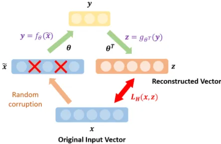
Figure 2.9: Training a single layer of denoising autoencoder. Input vectorxis corrupted to obtain
˜
x. The objective is to learn the parameter θ that is able to reconstructz from a compressed representation ofx˜ such that the error betweenz andx is minimized. The same parameterθ is used in both the encoding and the decoding phase.
Formally, an encoder is a deterministic mapping denoted by fθ (parameterized by model
parameterθ={W, b} where W andb are the weights and biases) transforms the input vector
x into a representation y. The decoder inversely maps the hidden representation y into the reconstructed input zwith the function gθT. The idea is to learn the model parameters θfor
both mappings such that the errorLH(x, z) between the reconstructed input and the original
input is minimized. Suitable loss functions could be cross-entropy loss with an affine-sigmoid decoder, or the mean squared error (MSE) loss with an affine decoder.
A denoising autoencoder performs an additional step on the input vector xby applying a salt-and-pepper noise to formx˜. In other words, some elements in the vectorxare randomly set to be zero. Therefore, in addition to learning a compressed representation of the input, a denoising autoencoder tries to further recover the clean input from the noisy input. It has been shown in [145] that applying a random corruption to the input will enable more robust extraction of features. x 1 1T x 1 2T 2 x 1 3T 2 3 x 1 2 3
(a) Training the first layer
(b) Training the second layer
(c) Training the third layer
(d) Trained SAE
Figure 2.10: Stacking multiple autoencoders to form a deep architecture. The layers are trained separately.
Autoencoders can be stacked on top of each other to form a deep architecture. After learning the encoding function of the first layer, the subsequent layers can be trained in a layer-wise manner while keeping the parameters of the previous layers fixed. This process is repeated for all layers in an unsupervised manner to extract robust features from the training set. When the procedure has been completed, supervised learning can take place by training the entire network by treating it as a regular DNN or adding an SVM classifier/logistic regression on top.
2.2 Regularization
In this subsection, we discuss some regularization techniques used in our research to combat the problem of overfitting. When a model overfits, the generalization power of the model to make inference based on unseen data is greatly reduced. An overfitted neural network is capable of reproducing even the finest details of noise in the input dataset. In other words, the bad model reproduces a non-smooth function corresponding to the non-smooth nature of the noise. As another method to combat overfitting, here we will also introduce the early stopping algorithm to the readers.
2.2.1 Weight decay x y x y x y x y x y x y (a) Perfect network (b) Overfitting, no regularization (c) Some regularization
(d) Optimal decay (e) Underfitting – regularization parameter too high
(f) Infinite regularization
parameter Estimate
Figure 2.11: Effects of varying regularization parameter. Panel (a) shows a perfect network being the ideal case. Panels (b) to (e) shows what happens when the regularization parameterλ
is increased. Panel (f) shows the situation whereλ=∞.
Weight decay is a form of regularization (Fig. 2.11). In essence, the weights within a neural network are constrained such that no one weight parameter dominates the other to ensure a smooth output function. When performing weight decay, we can modify the loss function that is minimized during the training procedure. LetL denote the original loss function. The modified loss function,L˜ is therefore:
˜
L=L+λS
where λis the regularization parameter (a constant that controls the level of smoothing) and
S is the value obtained after a chosen function is applied on the weights. For example, in`2
regularization, the weight vector is squared. With the modified loss function, the optimizer penalizes the loss function if the model weights become too large. On the other hand, `1
regularization may achieve the same effect while possibly attaining sparsity–a situation where some of the weights become zero. Neurons with`1 regularization end up using a subset of the
most important inputs and refrains from using noisy inputs.
2.2.2 Early stopping
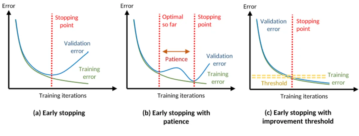
Early stopping is another form of regularization used to prevent overfitting when training a model using an iterative method such as stochastic gradient descent. This method is used in conjunction with cross-validation, where the training dataset is further split into a training set and a validation set. The model learns the parameters using the training set, and reevaluates
the model performance on the validation set after each update iteration. Generally, the training error will keep decreasing as the model is being trained. However, the plot of validation error will generally exhibit a U shape, meaning that at one point the validation error will keep increasing even though the training error continues to decrease (see Fig.2.12). When the errors diverge, the model is said to be overfitting. In early stopping, we select the saved model where validation error is at minimum. Training iterations Validation error Training error Error Stopping point Training iterations Validation error Training error Error Optimal so far Stopping point Patience
(a) Early stopping (b) Early stopping with patience Training iterations Validation error Training error Error
(c) Early stopping with improvement threshold
Stopping point
Threshold
Figure 2.12: The early stopping algorithm prevents overfitting by evaluating losses on both the training set and the validation set.
In some cases, the validation error may increase temporarily before decreasing again and signifies that the model has escaped bad local optima. Some algorithms include other user-defined parameters such as patience and improvement threshold that control how many iterations that the model should be trained. A large value for patience will allow the model to keep training for some extended time, even if the validation error continues to increase, with the hope that it will escape bad optima. On the contrary, it may be time-consuming to wait for the convergence of the validation error. The early stopping algorithm may stop training when the decrease in validation error is lower than the user-defined improvement threshold.
2.3 Feature visualization
One of the main claims of a hierarchical semantic feature extraction tool is that meaningful patterns in the data can signify the underlying characteristics of the process. Therefore,
visualizing the learned features is crucial to both understand and verify the performance of the feature extractor. Furthermore, intermediate feature visualization may lead domain experts to scientific discoveries that are not easy to figure out via manual exploration of large volume of data.
For the lowest layer in fully connected deep networks (e.g. DBN and DNN), plotting the weight matrix may be sufficient to visualize the features learned by the first hidden layer. Since the dimensionality of the input and the weights are in the same order, the vectors of weights for each input can be reshaped into the dimension equal to the resolution of the input image. Thus, the visualizations are usually intelligible. Complexity arises for visualizing features learnt at deeper layers because they lie in a different space from the visible data space. At the same time, the dimension of the weight matrix depends on the number of hidden units between the layer and the layer before. Thus, plotting the weight matrix will result in an incomprehensible visualization which typically resembles the appearance of white noise. To obtain filter-like representations of hidden units in the DBN, a recent technique known as Activation Maximization (AM) is used [38]. This technique seeks to find inputs that maximize the activation of a specific hidden unit in a particular layer and the technique is treated as an optimization problem. Letθ denote the parameters of the network (weights and biases) andhij(θ,x) be the value of the activation
function hij(·) (usually the logistic sigmoid function) of hidden unit i in layer j on input x.
Assuming the network has been trained,θremains constant. Therefore, the optimization process aims to find
x∗ = argmax
xs.t.||x||=ρ
hij(θ,x)
where x∗ denotes the inputs that maximizes the hidden unit activation. Although the problem is a non-convex optimization problem, it is still useful to find the local optimum by performing a simple gradient ascent along the gradient ofhij(θ,x) because in many cases, the solutions after
convergence are able to visualize the patterns of the inputs that are being learned by the hidden units.
In CNNs, learned features can be visualized by plotting the weight matrix of the feature maps in the same manner as obtaining filter-like representations from DNNs.
Summary. We have presented various deep learning architectures and regularization techniques that are used in our studies. The following chapters are dedicated to our pub-lished/submitted papers describing how we solve engineering problems with deep learning in detail along with additional results.