Modelling inclusion, testing and benchmarking of the impacts of ozone pollution on crop yields at regional level Module development and testing and benchmarking with the WOFOST generic crop model

(1)

EUR 28395 EN

Giovanni Cappelli Roberto Confalonieri Maurits Van Den Berg Frank Dentener

Modelling inclusion, testing and benchmarking of the

impacts of ozone pollution on crop yields at regional

level

Module development and testing and benchmarking with the WOFOST generic crop model

Report EUR XXXXX EN

(2)

This publication is a Technical report by the Joint Research Centre (JRC), the European Commission’s science and knowledge service. It aims to provide evidence-based scientific support to the European policy-making process. The scientific output expressed does not imply a policy position of the European Commission. Neither the European Commission nor any person acting on behalf of the Commission is responsible for the use which might be made of this publication.

Contact information

Name: Frank Dentener

Address: European Commission, Joint Research Centre, Directorate for Sustainable Resources, Via Enrico Fermi 2749, 21027 Ispra (VA), Italy

Email: [email protected] Tel.: +39 0332 78 6392 JRC Science Hub https://ec.europa.eu/jrc JRC103907 EUR 28395 EN

PDF ISBN 978-92-79-64945-5 ISSN 1831-9424 doi:10.2788/68501

Luxembourg: Publications Office of the European Union, 2016 © European Union, 2016

The reuse of the document is authorised, provided the source is acknowledged and the original meaning or message of the texts are not distorted. The European Commission shall not be held liable for any consequences stemming from the reuse.

How to cite this report: G. Cappelli, R. Confalonieri, M. Van Den Berg, F. Dentener; Modelling inclusion, testing and benchmarking of the impacts of ozone pollution on crop yields at regional level; EUR 28395 EN, Luxembourg: Publications Office of the European Union, 2016, doi:10.2788/68501

(3)

Abstract

The WOFOST crop model -as implemented in the BioMA modelling framework- was

extended with algorithms to account for the effects of ground-level ozone on crop growth and yield.

The additional algorithms implemented concern:

 Effect of water stress on stomatal conductance

 Reduction of carboxylation rate of Rubisco

 Ability of plants to partly recover from ozone damage

 Acceleration of leaf senesce due to O3 exposure

Meteorological datasets, with a consistent hourly-daily temporal resolution, were selected for two locations in Germany (Bremen) and Spain (Jerez), encompassing different climatic conditions. The sensitivity of two types of crops was assessed: wheat, which is relatively sensitive to O3 damage, and barley, which is less sensitive. These two crops were exposed to

a range of hypothetical O3 mixing ratios of 20, 40, and 60 ppb during the entire crop growth

cycle, as well as during specific months. Two agro-managements options were analysed: a potential yield case (i.e. no water stress by mimicking a full crop irrigation case), and a rain-fed case. Irrespective of ozone, rainrain-fed wheat and barley yields are lower by only 12 % in Bremen compared to fully irrigated crops, while strongly reduced by 55 % in Jerez. Additionally, wheat yield losses, up to 30 % are calculated for ozone concentrations of 60 ppb, and only half of these for barley. Yield losses are substantially smaller in Jerez for rain-fed crops, when stomatal closure is limiting gas exchange, and thus impeding photosynthesis, crop growth and yields, but also reducing ozone uptake.

General findings are:

 Crop damages due to O3 exposure increase with O3 concentration

 Effects of high O3 concentrations are very heterogeneous depending on month, site,

crop and the simulated variable considered

 The highest impact is obtained when the month with high O3 concentration coincides

with the anthesis/grain filling stage (June for Bremen, April for Jerez)

 Rain-fed crop damage is more marked in Bremen than Jerez and irrigation practice exacerbates O3 damages, especially in Jerez

 Barley is less affected by O3 impact according to the lower sensitivity of the crop.

The algorithms developed can easily be implemented in other (generic or crop-specific) models of similar complexity.

Compare model results against field data under diverse conditions will be the next phase of this work, and further model developments are needed to simulate so-called “stomatal

(5)

1. Introduction

Tropospheric ozone is a photochemically produced secondary pollutant whose precursors are nitrogen oxides (NOx), methane and other volatile organic compounds and carbon monoxide. There is a wealth of evidence that at ground level, ozone is phytotoxic to plants, and can cause substantial damage to crops [Mills et al., 2007; Ainsworth et al, 2012]. Empirical evidence and model-based assessments suggest a large impact on crop yields globally, yet with marked variations across regions and with intricate interactions with climate change impact, adaptation and mitigation actions [Van Dingenen, et al., 2009; Burney and

Ramanatan, 2014; Tai et al, 2014]. Ozone concentrations are already high in important crop-land areas in North America, Europe, and South and East Asia. Concentrations are increasing rapidly in developing countries and are projected to continue to increase in coming decades. However, the effects of ozone pollution are currently not considered in most crop models, including the WOFOST model, currently implemented in the BioMA framework, and used in the JRC MARS crop forecasting activity. Consequently, ozone effects are excluded from model predictions of regional crop growth and yield. A particular gap in our understanding is how ozone interacts with other stresses that effect crop growth, such as soil fertility,

CO2 fertilization, soil water stress, heat stress and even pests and diseases (e.g. ozone has been shown to make crops more vulnerable to attack by pests such as red spider mite). Nevertheless, there is sufficient information on the effect of ozone on crop physiology, particularly how it influences photosynthesis, C allocation and early senescence to warrant the development of ozone modules that could be embedded within existing crop models.

Based on the results of an expert contract with (Confalonieri, 2016) during the first semester of 2016, this report describes the work of experts from the University of Milano in

collaboration with JRC, to include ozone in the BioMA modelling framework, to integrate it with the WOFOST model and to provide detailed meteorological datasets for testing the models.

The report is structured as follows:

Section 2 describes which version of the WOFOST model was used for this study and for which reasons; and which interaction mechanisms between ozone and plant growth were included in the ozone module.

Section 3 describes the test conditions that were designed to evaluate the sensitivity of the extended model.

Section 4 describes the new ozone effect algorithms implement in the

Section 5 describes the results of the preliminary modelling experiments that were conducted for the test conditions described in section 3.

(6)

2. Selection of WOFOST version and interaction mechanisms to study

ozone effects on crops

Extensive experimental studies highlight the deleterious effects of chronic O3 exposure on

crop yields (Ainsworth et al., 2012). In such conditions, crop productivity is affected by a decreased CO2 assimilation at leaf level (Amax; e.g. Feng et al., 2008) and a decreased

synthesis of non-structural carbohydrates (i.e. sucrose, starch and pectins). These impacts on primary metabolism are partly responsible for the reduction of leaf area, a common response of field crops to O3 enriched air (e.g., Morgan et al., 2004; Pang et al., 2009). In

addition to lower carbon fixation, plants exposed to O3 often display i) higher respiration

rates (e.g., Amthor, 1988; Biswas et al., 2008), ii) altered biomass partitioning with decreased root biomass and redistribution of photosynthates from non-reproductive plant organs to grains and iii) a reduced leaf lifespan triggered by the acceleration of leaf senescence. All these responses contribute to the overall decrease in growth and yield. Interestingly, most of the processes affected are explicitly simulated by the WOFOST model (Diepen et al., 1989), which thus provides a suitable framework to integrate available models accounting for O3 limitations within a crop growth model. Currently,

two versions of WOFOST are implemented in BioMA (Stella et al., 2014; de Wit, 2014). They differ in the way by which they define the dependence of crop parameter values on air temperature and phenological development. The original WOFOST adopts so-called AFGEN tables to allow users to define arbitrary functions, which linearly interpolate between values of a dependent variable, Y, given a value of an independent variable, X, and a table of X and Y data pairs. In the new WOFOST-GT, such relations are described by simple mathematical equations, thus reducing model complexity and the number of parameters. Even though the second approach is deemed more elegant and sounder (since it reduces parameterization effort and the risk to fit unrealistic functions), we opted for using the original WOFOST which provides more flexibility and for which parameter sets are available which are widely used, including in the JRC MARS crop forecasting system. WOFOST is a generic crop simulator for annual field crops, based on a hierarchical distinction between potential and water-limited production. It performs its calculations with a one-day time step, using Euler integration to calculate the values of its state variables at the end of each day. Crop development rate is simulated as a simple function of temperature, photoperiod or both thermal and photoperiodic conditions. Photosynthesis (gross CO2 assimilation) is simulated on the basis of intercepted

photo-synthetically active radiation (PAR). Fluxes of direct and diffuse PAR are computed using Lambert-Beers law to estimate the light distribution in the canopy. The extinction

(7)

as a function of self-shading and senescence. A diagram showing the main processes accounted for by the WOFOST model and the possible coupling points to an idealised model reproducing the effects of O3 on plant growth is shown in Figure 1.

Figure 1. Flow chart of the processes implemented in the WOFOST model. Red stars indicate the processes that are subjected to ozone effects

Some adaptation to the model is required to enable consistent estimates of O3 damages. In the

BioMA framework, this is done within the so-called AbioticDamage component. An overview of adaptations considered is given in Table 1.

First, it is important to note that O3 damage largely depends on the flux of the gas into plant

tissues, which, in turn, is largely controlled by stomatal aperture. This means that either WOFOST or the O3 impact models that will be plugged into the modelling solution have to

calculate stomatal conductance (transpiration is using Penman- CO2 fluxes =H2O flux).

Although different models are available in literature (e.g. Leuning 1995; Medrano et al., 2002; Tuzet et al., 2003), the approach used by AquaCrop (Raes et al., 2009) seems to represent the best trade-off among the i) compatibility with the level of detail used by WOFOST to represent crop processes, ii) availability of input data usually stored in agrometeorological databases, iii) the availability of sets of proved parameters to differentiate crop-specific responses to water stress.

Moreover, even though WOFOST currently updates state variables with a daily time step, it could be important to estimate the O3 movement into the mesophyll (controlled by stomata)

at a shorter integration time step. The calculation of hourly fluxes could be a viable solution. The main reason for this is related to the diurnal variation of both O3 tropospheric

concentration – rising with high sunlight and temperature – and stomatal conductance, which are often coupled and sometimes decoupled (e.g., when excess light and temperature cause at the same time depression of photosynthesis and high O3 concentrations). This could be

managed by calculating, for all the groups of emitted GAI (green leave area index) units

Photosynthesis

Senescence

Leaf area index

Genotype coefficients Temperature

Radiation

Assimilates Conversion Partitio-ning Leaves Stems Repr. organs Roots Development rate Development stage (Daylength) Actual transpiration Potential transpiration Respiration _(repair of damage)

Model of crop growth and interaction with ozone

(Potential) Interaction with ozone.

(8)

having the same age, O3 fluxes at hourly time step in the range of the daylight hours and then

averaging the sum of hourly fluxes on the total number of contemporaneous age classes in the day. Daily averaged fluxes were then used to compute the O3-induced fractional reduction of

daily photosynthesis rates as simulated by WOFOST model. Another solution could be to convert WOFOST to hourly time step for all assimilation processes; which however was not yet possible with the time and resources allocated for this project. A case study comparing methods should be considered.

While O3 uptake depends on stomatal conductance, it is also known that O3 can affect

stomatal conductance. This can be a reducing effect (Morgan et al., 2003), probably because of the reduced photosynthesis and the related increase of CO2 concentration in the mesophyll,

or because of the formation of plant hormones in response to ozone, such as ethylene, which induces stomatal closure. Another key aspect in modulating stomatal conductance and O3

damages is water uptake: different experiments corroborate the hypothesis that drought mitigates the impact of O3 by causing stomatal closure, thus reducing O3 flux into leaves. On

the other hand, Wilkinson and Davies (2009) highlight an increasing effect, attributed to the loss of functionality of stomata in O3-stressed plants, which remain open despite drought

stress. This phenomenon, often referred to as ozone-induced stomatal sluggishness, has the potential to sensibly change the carbon and water balance of crops (Paoletti and Grulke 2005). Several approaches were inspected to understand their potential impact, were they to me implemented in the ozone model. The approach of Hoshika et al. (2015) (see table 1) appears to be promising but would require validation for its applicability to annual crops prior to its implementation.

Ozone is usually detoxified in plants at uptake rates below a critical threshold, above which the rate of photosynthesis decreases. The ability of crops to resist to low ozone concentrations via detoxification and repair is strictly dependent on leaf age (Alsher and Amthor 1988), with young leaves being able to tolerate higher O3 concentrations and completely repair from

damage in a relatively short time (from hours to days) depending on the cultivar and pedoclimatic conditions (Pell et al., 1997). Nevertheless, prolonged exposure to even low O3

concentrations is responsible for enhancing rates of leaf senescence, thus reducing the period during which plants can recover from ozone damage.

In any case, reliable estimates of drought stress and its impact on stomatal conductance requires the simple single-layer soil-water-plant-uptake approach of the WOFOST model to be replaced by a more elaborated soil water redistribution and uptake model; for example those implemented within the software component UNIMI.SoilW. For this study we decided to adopt:

 A multi-layer cascading approach (Ritchie, 1998) to simulate the downward movement of water through the soil profile: water fills up the layers until field capacity is reached, with the fraction exceeding this threshold moving to the deeper

(9)

Table 1. Inspected biophysical processes, model approaches and modifications needed to couple the original approaches to the BioMA AbioticDamage O3 model. I:

implemented; NI: not implemented.

Biophysical process Model approaches and modifications Action 1.2.1.1.1.1.1 Effect of

water stress on stomatal conductance

1.2.1.1.1.1.2 A water stress related factor that multiplies the stomatal conductance (0 =maximum reduction; 1 = no effect) is introduced in the algorithm computing O3 fluxes already implemented in the original O3 model available in the AbioticDamage component. following the approach used by AquaCrop (Raes et al., 2009).

1.2.1.1.1.1.3 I

Reduction of carboxylation rate of rubisco

According to Ewert and Porter (2000). Decreases in rubisco-limited rate, distinguish between i) immediate effects due to high ozone fluxes and ii) long terms effects driven by leaf senescence acceleration. Since decreases in daily rate of gross photosynthesis are implicitly induced by the reduction in GAIs associated to the faster ageing of each contemporaneous class of GAI units, the average long-term reducing factor will not be applied to further reduce the actual daily gross CH2O assimilation rate calculated by WOFOST. The rationale for this is to reduce the risk of markedly overestimating the effect of senescence on reducing photosynthesis rates, double counting its impact on plant growth. 1.2.1.1.1.1.4 I 1.2.1.1.1.1.5 Ability of plants to recover from ozone damage

According to Ewert and Porter (2000), the recovery from ozone-induced damage in a given day is used to modulate the ozone impact on rubisco-limited rate of photosynthesis at light saturated conditions of the following day, depending on leaf age. Since WOFOST considers LAI emitted units, instead of individual leaves, recovery factors are computed each day for all LAI units with the same age.

I

Metabolic cost (Increased respiration) to avoid or repair ozone damage

(10)

1.2.1.1.1.1.6 Acceleration

of leaf

senescence due to O3 exposure

1.2.1.1.1.1.7 Enhanced rates of senescence induced by prolonged exposure to O3 in a given day is computed daily for each GAI unit of the same age class using reducing factors (0 = maximum reduction; 1 = no effect; unit less) calculated as function of cumulative ozone uptake(Ewert and Porter, 2000). An average indicator targeting the shortening of leaves lifespan due to ozone exposure is computed by averaging the sum of all daily factors on the total number of contemporaneous GAI age classes.

1.2.1.1.1.1.8 I 1.2.1.1.1.1.9 Reduction of green leaf area index due to foliar chlorosis or necrosis induced by O3

1.2.1.1.1.1.10 An extensive literature search needs to be carried out to find out approaches that are i) coherent (neither too rough nor too refined) with the level of detail used by WOFOST and O3 models and ii) use standard input variables. As an alternative, if measured data are available from literature, one could derive generic response functions triggered by a crop–specific sensitivity parameter set to 0 (or to 1) in case of no impact.

1.2.1.1.1.1.11 N I

1.2.1.1.1.1.12 Stomatal sluggishness

1.2.1.1.1.1.13 The approach from Hoshika et al. (2015) accounts for the effect of chronic exposure to ozone on stomatal sluggishness by progressively increasing the minimum crop-specific stomatal conductance via a sigmoid function having the cumulative ozone uptake as independent variable. This model, as is, cannot be coupled directly with the AbioticDamage ozone model; but its implementation could be considered to modulate for instance the instantaneous O3 leaf uptake over a plant-specific threshold (UO>FO3crit)

1.2.1.1.1.1.16 N I

(11)

absence of O3; gminS (mol m−2 s−1) is the minimum stomatal conductance accounting for stomatal sluggishness as computed by Hoshika et al. (2015). 1.2.1.1.1.1.15 A strong limitation of Hoshika’s

approach is an empirical relationship developed for temperate deciduous forests and thus needs to be validated against measured data on herbaceous crops before being used outside the conditions for which it was calibrated.

(12)

3. Test conditions to evaluate the sensitivity of the modelling solution to

ozone exposure

A set of synthetic test conditions was generated to assess the crop model response in a range of environmental conditions for different crops, to verify model behaviour and to allow intercomparison with other models.

A first set of simulations was set up for two winter cereals with distinct tolerance to O3 and

environmental characteristics (such as different O3 atmospheric concentrations). The two

crops considered markedly differ in the sensitivity to ozone damage - i.e. winter wheat (susceptible) and winter barley (tolerant) – but share many phenological and productive traits1. This approach will greatly facilitate the analysis of results, allowing to separate the effects of O3 exposure on crops from any possible interference due to interspecific

differences in crop development and growth. Simulations were performed for two locations: 1) Bremen, in northwestern Germany, with a marine temperate humid climate and high yield potential, and 2) Jerez de la Frontera, Spain with Mediterranean climate with average-low yield potential. For each region, 20-years time series of meteorological data were selected [Table 4] to run simulations under rain-fed as well as under fully irrigated conditions. In this way, the potential interaction of ozone with drought conditions is explored (e.g., Morgan et al., 2003; Feng et al., 2008). Furthermore, such sample size is deemed large enough to capture the short-term random fluctuations – such as daily weather variations –, seasonal and interannual variability, as well as most part of the less frequent climate events that may occur in a given agro-ecosystem (Semenov and Barrow 2002). In this context simulations are performed by considering a sandy-loam soil, with a relatively low water holding capacity. Two reference levels of ozone concentrations are chosen: a sustained (without any daily or monthly variation) background ozone of 40 ppb and an elevated ozone of 60 ppb, respectively representative for background (inflow) O3 and elevated continental O3

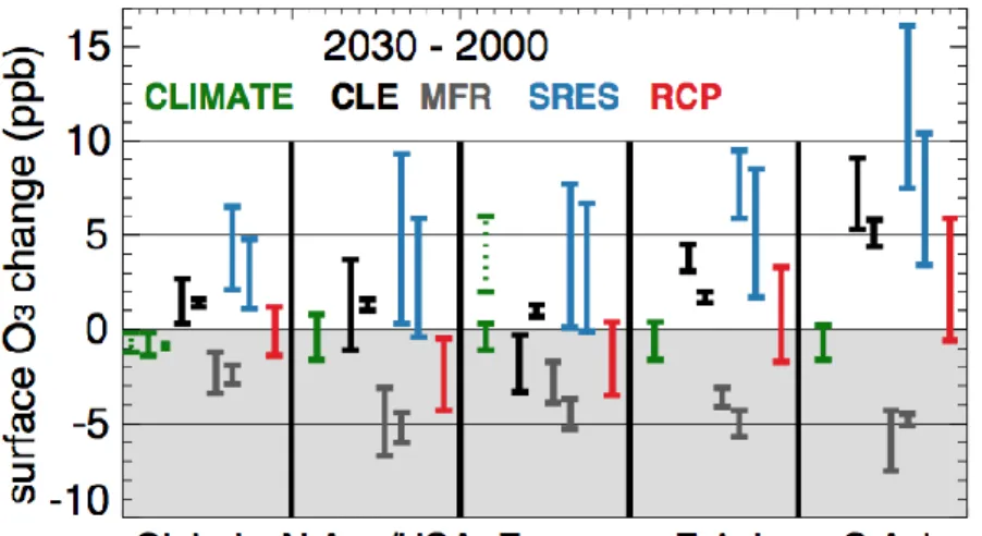
concentrations (Feng and Kobayashi, 2009). As current model calibrations may implicitly include some effect of ozone in the parameterization, simulations were also performed using a pre-industrial ozone concentration – i.e. 20 ppb – as reference control, to test the model in presence of negligible ozone damages. For this first analysis synoptic and diurnal variations of ozone are ignored, as they may complicate the analysis. We note that this range also encompasses future (2030) annual ozone levels under a variety of scenarios for 2000-2030- with projected regional changes ranging from ca. -8 to +15 ppb - depending on scenario and region considered (Figure 2; Fiore et al., 2012; Kirtman et al., 2013).

(13)

Figure 2. Changes in surface O3 (ppb) between year 2000 and 2030 driven by climate alone (CLIMATE, green) or driven by emissions alone, following current legislation (CLE, black), maximum feasible reductions (MFR, grey), SRES (blue) and RCP (red) emission scenarios. Results are reported globally. Where two vertical bars are shown (CLE, MFR, SRES ), they represent the multimodel standard deviation of the annual mean based on the Atmospheric Composition Change: a European Network (ACCENT)/Photocomp study (Dentener et al., 2006) and (right bar) the parametric HTAP ensemble (Wild et al., 2012; four SRES and RCP scenarios included). Under Global, the leftmost (dashed green) vertical bar denotes the spatial range in climate-only changes from one model (Stevenson et al., 2005) while the green square shows global annual mean climate-only changes in another model (Unger et al., 2006). Under Europe, the dashed green bar denotes the range of climate-only changes in summer daily maximum O3 in one model (Forkel and

Knoche 2006). Source Kirtman et al., 2013 in IPCC-AR5 report.

In addition to examining the effects on crop growth and yield of constant ozone concentration throughout the growing season, we also tested the model response to monthly variations in O3

concentration. For this purpose all months are set at the background ozone level (i.e. 40 ppb), except one, which is set at high ozone concentration (i.e. 60 ppb). Simulations are performed iteratively by changing each time the month displaying high O3 concentrations, in order to

identify the most critical phases of the crop cycle with regards to ozone exposure. The synopsis of the conditions explored is provided in Table 2; the total number of simulations (56) is determined by all the possible combinations of the factors and levels tested.

(14)

Table 2. Factors and levels tested in the first phase of the simulation experiment. Total number of simulation is 64.

Factor Levels

Crop Winter C3 (wheat, barley) O3 susceptibility Tolerant (winter barley)

Susceptible (winter wheat)

Climate Marine

Mediterranean

Precipitation Rainfed

Full irrigated Soil texture Medium/sandy-loam

20 whole cycle O3 concentration (ppb) 40 whole cycle

60 whole cycle 60 February 60 March 60 April 60 May 60 June

For each combination of conditions tested, selected model output is stored (Table 4) to gain insight into the modelled effect of ozone damage on crop growth and productivity. In particular, daily values of aboveground biomass, green leaf area index and storage organs biomass are used as key variables influenced by photosynthesis activity. Variables related to water use, such as daily and cumulative evapotranspiration and water stress index (i.e., the ratio between potential and actual transpiration), are used to distinguish the impacts of losses due to water stress and stomatal closure from the losses due to ozone exposure. Final yield, harvest index and total water use are chosen as the synthetic variables describing crop productivity. Furthermore daily and cumulative O3 fluxes to stomata and the percentage

reduction of daily assimilation rates are tracked to separately inspect the effects of short- and long-term exposure to O3. A summary of data needed as input for the modelling solution and

(15)

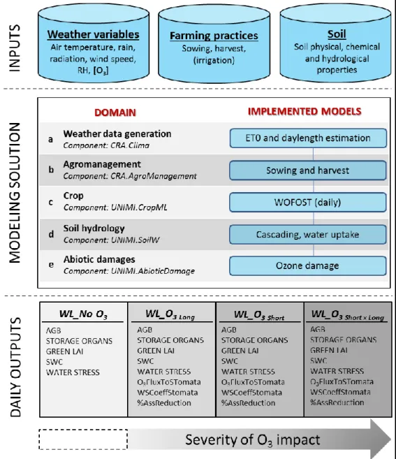
Table 3. List of inputs needed to run the modelling solution under the test conditions defined in Table 1. Inputs are grouped in three classes, related to i) daily meteorological data, ii) crop management data and iii) Soil properties initialization data.

Inputs Unit

Daily meteorological data

Maximum air temperature °C

Minimum air temperature °C

Cumulative precipitation mm

Average wind speed mm s-1

Minimum relative air humidity %

Maximum relative air humidity %

Global solar radiation MJ m-2 d-1

Reference evapotranspiration mm

Latitude °

Tropospheric Ozone concentration ppb

Crop management data

Sowing date doy

Irrigation starting date doy

Harvest date doy

Soil properties initialization data

Horizon thickness m

Volumetric water content at saturation m3 m-3

Volumetric wilting point m3 m-3

Volumetric field capacity m3 m-3 Saturated hydraulic conductivity mm h-1

Bulk density t m-3

Texture* %

Number of layers -

Layer thickness m

Skeleton %

(16)

Table 4. List of simulated outputs analyzed. Variables are grouped in three classes, related to i) water management, ii) crop productivity and iii) ozone damage to crop.

Simulated output Unit

Water management

Daily ET0 mm d-1

Cumulative ET0 mm

Water stress index -

Water stress effect on stomatal conductivity -

Crop productivity

Daily aboveground biomass kg ha-1

Daily green leaf area index m-2 m-2

Final yield kg ha-1

Harvest index -

Cumulative water uptake mm

Ozone damage

Instantaneous O3 fluxes to stomata nmol m-2 s-1

Cumulative O3 fluxes to stomata nmol m-2

Percentage Amax reduction %

ET0: reference evapotranspiration; Amax: maximum leaf

CO2 assimilation rate (Kg ha-1 h-1), WOFOST parameter.

In order to identify eligible test sites where to perform the first phase of simulation experiment, we crossed the information from the i) European climate classification according to the Köppen-Giger taxonomy (Figure 3; Peel et al., 2007), ii) maps of wheat and barley production area coverage and productivity by country (Figure 4; Bioma, 2016; FAOSTAT 2016), iii) the within country percentage cover occupied by selected species (USDA 2016), iv) the presence of reliable, consistent and accessible data sources, able to provide long time series of meteorological data, essential as input for the modelling solution.

(17)

Figure 3. Map of European climate and sites selected as representative for Marine and Mediterranean climates.

As result, data from meteorological stations located close to Bremen, in northwestern Germany, and to Jerez de la Frontera, in south-western Spain, were selected as representative for Marine and warm Mediterranean climate. By analyzing data on the average production quantities by country available in the FAOSTAT database in the period 1993-2013, both countries prove to be among the top wheat and barley producers in the EU-27 (Figure 4).

Figure 4. Crop area- production area for wheat and barley (http://bioma.jrc.ec.europa.eu). Red circles represent the sites selected to run the first set of simulations.

(18)

The economic importance of the two winter cereals in the target sites is confirmed by the high percentage of wheat and to a smaller extent barley harvested area in the region/state of belonging (Figure 4).

It can be noticed that the selected crops markedly differ in the average yields achieved, according to the crop suitability to pedo-climatic conditions in the target areas. While yields in Niersachsen, around Bremen, fluctuate around 7.5 t ha-1 (± 0.52 tha-1) for wheat and 6.0 ha

-1

(± 0.54 tha-1) for barley, in Andalucia (Jerez de la Frontera) both crops show average yields of about 2.9 t ha-1 with a standard deviation ranging from 0.49 t ha-1 to 0.57 tha-1.

For both sites, daily maximum and minimum air temperature (°C), precipitation (mm), average wind speed (m s-1) and relative air humidity (%) were extracted from the European Climate Assessment & Dataset (ECA&D; http://eca.knmi.nl/). Global solar radiation (MJ m-2 d-1) and reference evapotranspiration (ET0; mm) were generated according to Hargreaves

(Hargreaves and Samani 1982) and FAO (Allen et al., 1998) equations respectively. The monthly patterns of meteorological variables collected within the period 1996-2015 were then analyzed; some synthetic previews are shown in Appendix (Figure 1 and 2). In addition, the above listed daily data were used to generate hourly values of meteorological drivers, in order to produce an hourly meteorological dataset consistent with the daily one, to be used as input to the hourly time step O3 models for future intercomparisons. To generate synthetic

hourly data, the following approaches were adopted:

 hourly air temperature: Campbell (1985);

 hourly air relative humidity: Waichler and Wigmosta, 2003;

 hourly wind speed: Mitchell et al., 2000;

 hourly rainfall: Meteotest 2003;

 hourly radiation: Chen et al., 1999;

 hourly reference evapotranspiration: Allen et al., 1998.

An overview of weather variables patterns in both sites is given in Appendix A.

Options for future work:

Once results will be definitive, the reference simulation protocol could be reiterated on the same crops by changing soil texture and/or adopting more realistic patterns of monthly mean surface ozone concentrations (e.g., Avnery et al., 2011). As an alternative, the setup of simulation experiment could be applied to other C3 species or even to C4 summer crops (extending to September), which generally show a lower sensitivity of plant growth to O3

(19)

4. The modelling solution and modifications to the AbioticDamage

component

4.1.The modelling solution

The third phase of the workflow dealt with the realization of a customized modelling solution for the simulation, with daily time step, of ozone (O3) damages to crops The developed

modelling solution links (i) the original WOFOST version implemented in the software component UNIMI.CropML, (ii) soil water redistribution and uptake models collected by UNIMI.SoilW and (iii) the amended ozone impact model present in UNIMI.AbioticDamage (Figure 5).

Figure 5. Schematic representation of the models composing the modelling solution and the components they belong to.

The CropML_SoilW_AbioticDamage_solution project handles the interactions between the I/O data produced by models belonging to the software components, in order to simulate the

(20)

different biophysical processes shown in Figure 5. The entry point of the modelling solution is the RunnerAPI class, containing instances of Adapter classes (Gamma et al., 1994) and managing their call. Adapter classes, in turns, encapsulate the logic to perform dynamic simulations, by calling specific models selected among those provided by software components. The components implemented in the modelling solution communicate in each integration time step (daily), via the methods provided by ISimulationComponent interface. Information produced during the simulation is stored in dedicated classes i.e., DataTypes, containing the instances of the data structures of the components implemented in the modelling solution. DataTypes are also used to store input data from different sources (e.g., meteorological data, pedological information). All DataTypes are shared by all the Adapter classes of the MS, making possible the communication of models belonging to different domains, meant as the possibility of exchanging variables among software components. The Adapter class of the component CRA.AgroManagement is able to publish specific events (e.g., planting, harvest), which are listened by other Adapters via the HandleEvents method of the ISimulationComponent interface.

4.2.Input data layers

The data needed as inputs to the CropML_SoilW_AbioticDamage_solution are organized in information layers and integrate data from different sources, allowing an ease coupling with biophysical models.

 Weather layer contains .txt files collecting daily meteorological data covering the whole simulation period for the site to be tested. Weather variables included in the sample weather file used to test the modelling solution are the following: daily minimum and maximum air temperatures (°C), rainfall (mm), average wind speed (m s-1) global solar radiation (MJ m-2 d-1) minimum and maximum relative humidity (%) and Ozone concentration (parts per billion, ppb).

 Farming practices layer is represented by a single .xml file which currently includes the crop species grown, the sowing and harvest date and the planting depth for each combination site × year. This layer can be modified and/or extended by the user by specifying different sets of rules and impacts to simulate alternate management strategies.

 Soil layer is made up by an .xml file collecting the parameters to set the physical and hydrological properties along the soil profile at the beginning of simulation. Main soil properties concern: horizon thickness (m), volumetric water content at saturation (m3 m

-3

), volumetric wilting point (m3 m-3), volumetric field capacity (m3 m-3), saturated hydraulic conductivity (mm h-1), bulk density (t m-3), texture (i.e. relative percentage of clay, silt and sand; %), skeleton (%), number of layers (unit less) and layer thickness

(21)

angle and a correction parameter specific for each day of the year. Day length is estimated as function of latitude and solar declination.

b. CRA.AgroManagement triggers the occurrence of agricultural operations at run time according to (i) set of rules based on management decisions (e.g., scheduled events) and/or some states of the system. This components currently handles – within the solution – sowing and harvest operations, with the possibility of including dedicated rules to manage irrigation events according to the method (e.g. sprinkler, surface flow, drip or flood irrigation) and the scheduling time needed (i.e. turn or plant needs based irrigation). For instance, the fully irrigated treatment as defined in the test condition report (no stress due to water shortage), was reproduced here according to an automatic rule which triggers an irrigation event every time that the water stress index is lower than one, bringing the volumetric soil water content in the rooted soil back to field capacity.

c. UNIMI.CropML implements the model WOFOST. Crop development is simulated as a thermal-driven process. Instantaneous gross CO2 assimilation is estimated in three

moments during the day as a function of intercepted radiation and of a photosynthesis-light response curve of individual leaves. Light interception depends on total incoming radiation, on photosynthetic leaf area and on leaf angle distribution. Canopy architecture is divided into three horizontal layers with LAI split among them using Gaussian integration. Biomass partitioning is driven by partitioning factors and efficiencies of assimilates conversion into the different organs (i.e., growth respiration). Daily increase in total LAI is estimated as a function of temperature during early growth whereas it is derived from specific leaf area and development stage later on. Non-photosynthetically active (dead) LAI units are computed each day as a function of canopy self-shading and senescence. Potential evapotranspiration is estimated using the Penman approach (Frere and Popov, 1979), and water stress is derived by the actual to potential transpiration ratio. d. UNIMI.SoilW is used to simulate soil water redistribution among soil layers according to

a cascading (tipping bucket) approach. The changes of soil water content and fluxes among layers are provided as output; water percolating from the bottom layer is lost from the soil column. The component also estimates root water uptake based on evapotranspiration demand, soil water content and variable root depth. The component does not simulate water infiltration. Input water is assumed to be net rain able to infiltrate the soil. No attempt to compute runoff, plant and mulch interception is performed. The component also allows the simulation of effective plant transpiration, soil evaporation and the effects of soil tillage and subsequent settling of hydrological properties of the soil (field capacity, wilting point, retention functions, conductivity functions, bulk density). The latter are not taken into account in the current modelling solution.

e. UNIMI.AbioticDamage contains a complex model for the simulation of the crop damages due to ozone. It implements a model of leaf aerodynamic and boundary layer resistance (Spiker et al., 2007), the calculation of average leaf conductance proposed by Georgiadis et al. (2005), and the fractional reduction of plant production in function of the ozone flux through the stomata and the leaf conductance of water, according to the approach proposed by Sitch et al. (2005).

4.4.UNIMI.AbioticDamage modifications

As discussed in section 2 of this report (Selection of WOFOST version and interaction mechanisms to study ozone effects on crops), the O3 model implemented in the

UNIMI.AbioticDamage component has been modified to account for some O3 effects on crop

(22)

4.4.1. Effect of water stress on stomatal conductance

A water stress related factor modulating the stomatal conductance (Ks, 0 =maximum

reduction due to water stress-induced stomatal closure; 1 = no effect; unitless) was introduced in the algorithm computing the instantaneous O3 leaf uptake over a critical threshold

(UO>FO3crit; Equation 1, Sitch et al., 2005) to adjust O3 fluxes to stomata (FO3, nmol m-2 s-1).

[1]

Where: FO3crit , (nmol m-2 s-1) is a plant-specific critical threshold below which the damage to

tissues due to O3 leaf uptake is equal to 0. In other words, the lower the threshold, the higher

is the plant susceptibility to O3 damage.

Ks response function is computed according to the approach used in the model AquaCrop (Equation 2; Figure 5; Raes et al., 2009).

[2]

Where: Drel (%) is the fraction of water depleted in the root zone relative to the full amount

the soil can hold between an upper (pupper) and lower (plower) critical threshold of total

available soil water (TAW); fshape (unit less) is a crop specific parameter modulating the

shape of the response curve (e.g. 2.5 for wheat, 6 for maize and sorghum, 3, for rice, potato and soybean, 2 for sunflower).







,

0 

max

₃ ₃

3crit s crit

FO

K

FO

UO

_







UO

__FO₃_crit



max





FO

₃



K

_s



FO

₃_crit



,

0 





















1

0

1

1 Drel

if

Drel

if

Drel

if

sh a p e sh a p e rel f f D s

e

K

(23)

The critical thresholds are expressed as a fraction of TAW, with the lower one set to permanent wilting point (plower=1); Drel is computed according to equation 3.

[3] Where: FC (m3 m-3) is the volumetric soil water content at field capacity; WC (m3 m-3) is the actual volumetric soil water content in the rooted zone; WP (m3 m-3) is the volumetric soil water content at wilting point.

Tabular values for the upper threshold (p) are given for different crops at a reference evaporative demand of ET0 = 5 mm d-1; for different levels of ET0, pupper is adjusted at

runtime according to the equation 4 (Raes et al., 2009).

[4]

Where: fadj (unit less, default value = 1) is a model parameter set to increase (>1) or decrease

(<1) the pupper adjustment.

The log term in the equation 4 amplifies the adjustment when the soil is wet compared to when it is dry, based on the likely restriction of stomata and transpiration (and thus a lower effect of the evaporative demand) when the soil is dry.

4.4.2. Reduction of daily rate of gross photosynthesis

The library of O3 impact models on photosynthesis rates implemented in

UNIMI.AbioticDamage component (Sitch et al., 2005) was extended by including the approach developed by Ewert and Porter (2000), which models the decreases in the hourly rates of net photosynthesis distinguishing between (i) immediate effects due to high ozone fluxes and (ii) long term effects driven by leaf senescence acceleration. In order to allow the new ozone impact model based on thea SUCROS approach of photosynthesis (Van Ittersum et al., 2003), originally developed for Farquhar (Farquhar et al., 1980),) we applied the ozone damage factors to reduce the actual daily gross CH2O assimilation rate, as driven by the

maximum leaf CO2 assimilation rate (Amax, Kg ha-1 h-1 ) limited by temperature and solar

radiation absorbed by the shaded and sunlit leaves. Since the WOFOST model considers the Green Area Index (GAI) emitted units, instead of leaves surface, both short- and long-term effects are computed each day for all the groups of emitted GAI units having the same age and then averaging the sum on the total number of contemporaneous age classes.

4.4.2.1. Short-term response and ability of plant to recover from ozone damage

The short-term O3 effect on photosynthesis is computed daily for all GAI units of the same

age class using a short-term hourly damage factor (GAI_fO3,s(h), 0 = maximum reduction; 1 =

no effect; unit less) calculated, for each daylight hour, using a linear relationship between ozone uptake and the daily rate of gross photosynthesis (Equation 5; Figure 6; Ewert and Porter, 2000).). upper upper rel

p

WP

FC

WC

FC

D



















1

_upper upper rel p p WP FC WC FC D            1







0.04 5



log



10 9



1

(24)

[5]

Where: UO>FO3crit (nmol m-2 s-1) is the instantaneous O3 leaf uptake rate (Equation 1); γ1 (unit

less; default = 0.06) and γ2 ((nmol m-2 s-1)-1; default = 0.0045) represent short-term damage

coefficients empirically determined.

Figure 6. Relationship between factor accounting for short-term ozone effect on the daily rate of gross photosynthesis (GAI_fO3,s(h)) and ozone uptake.

Hourly damage factors (GAI_fO3,s(h)) computed for daylight hours are then aggregated in a

daily reduction factor (GAI_fO3,s(d)) for GAI units of the same age, considering both the

damage caused by ozone during the previous hour (GAI_fO3,s(h-1)) and recovery from ozone

injury of the previous day (GAI_rO3,s), as shown in Equation 6.

[6] Where: a (h) is the first sunshine hour in the day; n (h) is the total number of sunshine hours in the day.                       2 1 3 2 1 3 2 1 3 2 1 2 1 3 s(h) 3, 1 1 0 1 1 O _           crit FO crit FO crit FO crit FO UO if UO if UO if UO f GAI           1 1 ... 1 s 3, s(h) 3, 1) -s(h 3, s(h) 3, s(d) 3, O GAI_ O _ O _ O _ O _ h for n a h for r f GAI f GAI f GAI f GAI

(25)

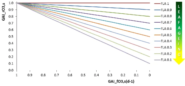
Figure 7. Recovery rates ozone injury factor (GAI_rO3,s,unitless) as function of the short-term daily

damage factors of the previous day (GAI_fO3,s(d), unitless) and leaf age (GAI_fLA, unitless).

While young leaves can fully repair from O3 damage, the recover capacity decreases linearly

with the ageing of the leaves up to zero when the leaf is dead (Equation 8; Figure 8). [8]

Where: GAI_PHYSDEL (d) represents the physiological age of a representative leaf belonging to a given GAI unit; GAI_SPAN (d) is the life span of a representative leaf belonging to a given GAI unit.

             SPAN GAI PHYSDEL GAI if SPAN GAI PHYSDEL GAI if SPAN GAI PHYSDEL GAI PHYSDEL GAI if f GAI _A _ _ 0 _ _ 0 _ _ 1 0 _ 1 _ _L

(26)

Figure 8. Relationship between factor used to simulate the recovery from ozone damage dependent on leaf age (GAI_fLA) and the thermal life-span of a representative leaf belonging to a given GAI unit.

An average short-term daily effect (Average_GAI_fO3,s(d)) is computed by averaging all daily

reduction factors (GAI_fO3,s(d), specific for each contemporaneous GAI unit) and is then

applied to reduce the gross photosynthesis rate calculated by WOFOST.

[9]

Where: DGAR (Kg ha-1 d-1) represents the actual daily gross CH2O assimilation rate.

4.4.2.2. Long-term response and acceleration of leaf senesce due to O3

exposure

Both the signal for the onset of senescence and the rate of senescence are computed daily for each contemporaneous GAI unit using reducing factors (GAI_fO3,l, 0 = maximum reduction;

1 = no effect; unit less) calculated as function of cumulative ozone uptake (Equation 10). [10]

Where: γ3 ((μmol m-2)-1; default = 0.5) is an ozone long-term damage coefficient, empirically

determined, describing the reduction in the lifetime of a mature leaf per unit of ozone accumulated uptake; UO>FO3crit (nmol m-2 s-1) is the instantaneous O3 leaf uptake rate

(Equation 1); hdaylight (h) are the sunshine hours in a given day.

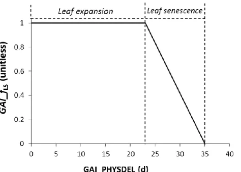
Then the factor accounting for the effect of leaf senescence on daily rate of gross photosynthesis (Figure 9) is calculated as,

[11]

Where: tl,ep = 0.33 GAI_SPAN (d) are the days during which a representative leaf belonging

to a given GAI unit is fully expanded.

s(d) 3, O I_ Average_GA f DGAR DGAR 



  _ 

 t GAI SPAN daylight crit FO l h UO fO GAI _ 0 3 3 , 3 1000 1 _                                            SPAN GAI PHYSDEL GAI if SPAN GAI PHYSDEL GAI t if t PHYSDEL GAI if ep l ep l l ep l ep l S t fO GAI SPAN GAI t PHYSDEL GAI f GAI _ _ _ _ _ 0 0 , _ _ _ 1 max 1 _ _, , , 3 , , L

(27)

Figure 9. Relationship between factor used to simulate the decline in the daily rate of gross photosynthesis in senescing leaves (GAI_fLS) and the thermal life-span of a representative leaf belonging to a given GAI unit

Finally, an average long-term daily effect (Average_GAI_fLS) is computed by averaging the

sum of all daily reduction factor (GAI_fLS) on the total number of contemporaneous age classes.

Since decreases in daily rate of gross photosynthesis are implicitly induced by the reduction in green leaf area indices (GAIs) daily associated to the faster ageing of each contemporaneous class of GAI units, the Average_GAI_fLS factor is not applied to further

reduce the actual daily gross CH2O assimilation rate calculated by WOFOST in the

modelling solution (Equation 9). The rationale for this is to reduce the risk of markedly overestimating the effect of senescence on reducing photosynthesis rates, double counting its impact on plant growth.

The effect of leaf senescence acceleration is computed daily in the ozone module by increasing the physiological age of all the contemporaneous GAI units (GAI_PHYSDEL) according to the Equation 12.

[12]

Where: GAI_SPANAdj(t) (d) is the life span of a given GAI unit modified by the ageing effect

of cumulative ozone; GAI_SPANAdj(t-1) (d) is the adjusted life span of the previous day.

Each day GAI_SPANAdj(t) is calculated via Equation 13 and then used to update the

WOFOST GAIage state variables of the following day.

[13]

The metacodes referring to the algorithms implemented for the short- and long-term effects are reported in Appendix B and C respectively.



_ _ ,0



max _

_PHYSDEL GAI PHYSDEL₍_t ₁₎ GAI SPAN_Adj₍_t ₁₎ GAI SPAN_Adj₍_t₎

GAI      l fO t Adj t

Adj GAI SPAN GAI

SPAN

(28)

4.5.Daily outputs

At the end of each simulation run, daily outputs of the CropML_SoilW_AbioticDamage_solution are stored in .xls files and can be displayed via the Graphic Data Display (GDD) user interface application ( http://agsys.cra-cin.it/tools/gdd/help/). Four different production levels are considered and results achieved for each of them are saved, separately in a dedicated sheet. This methodological choice allows to gain insight into the modeled effect of ozone damage on crop growth and productivity. The levels are:

1 WL_No O3: it takes into account just water stress limitations to crop growth without

considering any O3 influence on crop phenology and productivity. Main daily outputs

stored involve:

o above ground biomass (AGB; Kg ha-1);

o storage organs biomass (STO; Kg ha-1);

o green lai index (GAI; m-2 m-2);

o soil water content (SWC; m-3 m-3);

o water stress index (WSI; unit less);

o rooting depth (RD; m).

2 WL_O3 Long: it takes into account water stress limitations in conjunction with the O3

long-term effect on crop growth and leaf senescence. Short-term O3 effect is not

considered. Main daily outputs stored involve:

o AGB_Long (Kg ha-1);

o STO_Long (Kg ha-1);

o GAI_Long (m-2 m-2);

o SWC_Long (m-3 m-3);

o WSI_Long (unit less);

o RD_Long (m);

o O3 flux to stomata (O3FluxTOStomata_Long; nmol m-2 s-1);

o Effect of water stress on stomatal conductance (Ks_Long; unitless);

o Percentage reduction of daily CH2O assimilation rate (%AssReduction_Long;

%).

3 WL_O3 Short: it takes into account water stress limitations in conjunction with the O3

short-term effect on crop growth and leaf senescence. Long-term O3 effect is not

considered. Main daily outputs stored involve:

o AGB_Short (Kg ha-1);

(29)

o AGB_Short x Long (Kg ha-1);

o STO_Short x Long (Kg ha-1);

o GAI_Short x Long (m-2 m-2);

o SWC_Short x Long (m-3 m-3);

o WSI_Short x Long (unit less);

o RD_Short x Long (m);

o O3FluxTOStomata_Short x Long (nmol m-2 s-1);

o Ks_Short x Long (unitless);

o %AssReduction_Short x Long (%).

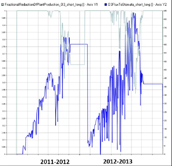
As an example, some results about the simulated impact of short- and long term O3 exposure

on wheat AGB and STO are presented in Figure 10, where two contrasting regimes of ozone concentration are compared.

Figure 5. Graphic Data Display (GDD) interface showing aboveground biomass (kg ha-1) and storage organs biomass (kg ha-1) of wheat (water limited, Long-term O3 limited, short term O3 limited and

with all limitations) simulated under two contrasting regimes of ozone concentration in a sample

site of Northern Italy (seasons 2011-2012 and 2012-2013) with the

CropML_SoilW_AbioticDamage_solution.

While crop productivity is slightly affected under the low-impact O3 concentration regardless

the production level considered, a decline in both AGB and STO up to -20:-25% is simulated under the enriched O3 scenario, with differences depending on the variable and production

level analyzed.

The percentage reduction of daily CH2O assimilation triggering the STO and AGB losses

under the highest O3 concentration are shown in Figure 11, where %AssReduction_Short x

(30)

Figure 6. Graphic Data Display (GDD) interface showing the percentage reduction of daily CH2O

assimilation rate (%, light blue) against O3 fluxes to stomata (nmol m-2 s-1; bue) simulated under

enriched O3 concentration (60 ppb) for the limited production level (seasons 2011-2012 and

2012-2013).

As it can be noticed, O3 fluxes to stomata frequently exceeded a threshold for damage in the

growing season 2012-2013 causing decreases in daily assimilation rate up to 60 %, whereas in 2011-2012 reductions in assimilation rates were mainly confined toward the end of the season. Daily fluctuations in O3 fluxes to stomata strictly depend on aerodynamic boundary

layer resistance and stomatal conductivity, as influenced by intercepted solar radiation, O3

effect and water stress.

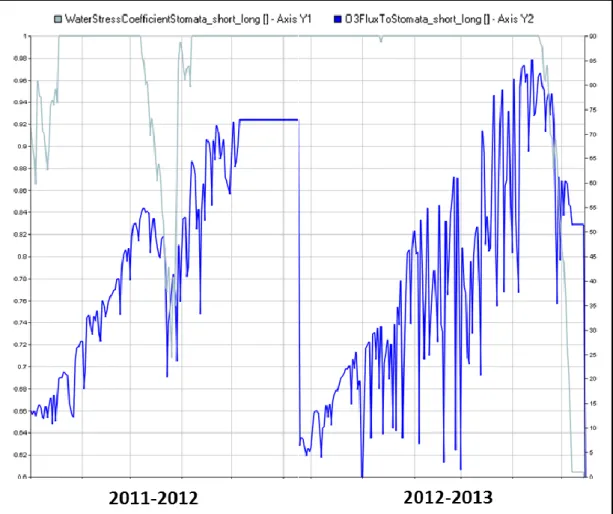
A picture of the effect of water stress on stomatal conductivity and its relationships with O3

(31)

Figure 7. Graphic Data Display (GDD) interface showing the effect of water stress on stomatal conductance (Ks_Long; unitless; light blue) O3 fluxes to stomata (nmol m-2 s-1; bue) simulated

under enriched O3 concentration (60 ppb) for the all limited production level (seasons 2011-2012

and 2012-2013).

The water stress-induced reduction of stomatal conductance simulated in the first part of the season largely contributed to protect the crop from O3 damage in 2011-2012, whereas in the

following season the crop had less benefit from this mechanism, due to the higher amount of rainfall and soil water content in the rooted zone (Figure 13).

(32)

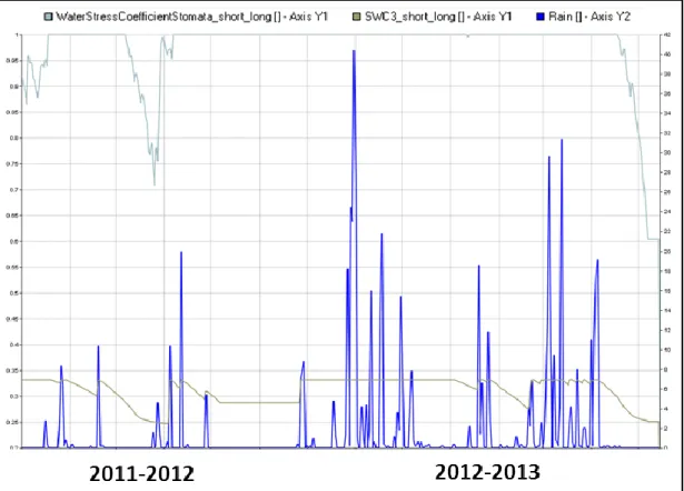
Figure 8. Graphic Data Display (GDD) interface showing the effect of water stress on stomatal conductance (Ks_Long; unitless; light blue), daily rainfall patterns (mm) and the soil water content in the rooted zone (mm) simulated under enriched O3 concentration (60 ppb) for the all limited

production level (seasons 2011-2012 and 2012-2013).

To conclude, a synthetic overview of possible fluctuations of O3 fluxes to stomata and of

percentage reduction of daily CH2O assimilation rate as function of the variation of ozone

short-term damage coefficients γ1 and γ2.(Equation 5) are shown in Figure 14; the flux of 90

(33)

Figure 9. Changes in the values of O3 flux to stomata (nmol m-2 s-1) and in the factor triggering the

reduction of daily CH2O assimilation rate (%) as function of different combinations of short-term

(34)

5. Preliminary results from the test conditions experiment

The preliminary results of the simulations to evaluate the sensitivity of the modelling solution to ozone exposure under the test conditions described in section 3 are reported below as:

 boxplots, to show the variability in the 20-years series of simulated outputs;

 daily dynamics, to highlight the differences in model behavior in contrasting growing seasons (e.g. high versus low impact years).

We note here, that the evaluation of the model results against observations, would need the evaluation of detailed chamber and field studies in a coherent way, which will be performed in different study.

While the seasonal outputs aim to highlight the differences among the short-, long- and short&long production levels (as explained in section 4.5) and the consecutive impacts of 03

damage on yield , the long-term simulations refer exclusively to the Short & Long production level and concern:

 final AGB (kg ha-1), final yield (kg ha-1) and maximum green leaf area index (m2 m-2) among the growth variables,

 number of days with O3 flux exceeding the critical crop-specific O3 concentration (d),

average fractional reduction of daily gross CH2O assimilation rate during the crop

cycle (%), the cumulative O3 fluxes during the growing season (nmol m-2) among the

variables triggering the O3 damages.

5.1.Long-term simulations under different tropospheric O3 concentrations

Figures 15-18, show yields for wheat and barley in Bremen and Jerez for different ozone conditions: 20 ppb (pre-industrial), 40 ppb (current background), and 60 ppb (polluted), the latter average over the growing season, or in specific months on top of the 40 ppb

background conditions. Irrespective of ozone, rainfed wheat and barley yields are lower by only 12 % in Bremen compared to fully irrigated crops, while strongly reduced by 55 % in Jerez. Additionally, wheat yield losses, up to 30 % are calculated for ozone concentrations of 60 ppb, and only half of these for barley. Yield losses are substantially smaller in Jerez for rain-fed crops, when stomatal closure is limiting gas exchange, and thus impeding

(35)

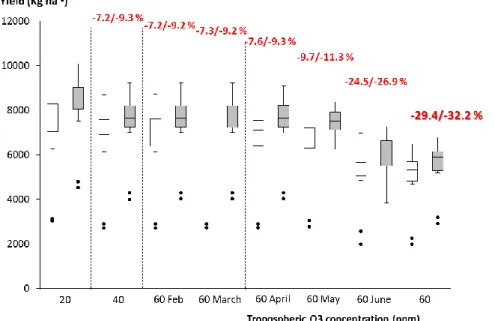
5.1.1. Final Yield

Figure 10. Boxplot of final yield values (kg ha-1) simulated for the pre-industrial, background and high ozone concentrations scenarios. Each box is derived from the 19 annual values simulated for wheat crop in Bremen, Germany. Open boxes refer to rainfed; grey boxes to fully irrigated conditions. Dots represent results for the two lowest extreme years. Red numbers represent the relative reduction due to ozone compared to the 20 ppb case.

Figure 11. Boxplot of final yield values (kg ha-1) simulated for the pre-industrial, back ground and high ozone concentrations scenarios. Each box is derived from the 19 values simulated for wheat crop in Jerez de la Frontera, Spain. Open boxes refer to rainfed conditions, grey boxes to fully irrigated conditions. Dots represent results for the two lowest extreme years. Red numbers represent the relative reduction due to ozone compared to the 20 ppb case.

(36)

Figure 17. Boxplot of final yield values (Kg ha-1) simulated for the pre-industrial, back ground and high Ozone concentrations scenarios. Each box is derived from the 19 values simulated for barley crop in Bremen, Germany. Open boxes refer to rainfed conditions, grey boxes to fully irrigated conditions. Dots represent results for the two lowest extreme years. Red numbers represent the relative reduction due to ozone compared to the 20 ppb case.

Figure 18. Boxplot of final yield values (kg ha-1) simulated for the pre-industrial (20 ppb), back ground (40 ppb) and high (60 ppb) Ozone concentrations scenarios. Each box is derived from the

(37)

Figure 19. Boxplot of absolute amounts of water (mm) applied to wheat/barley crops during the growing seasons under the fully irrigated conditions for the pre-industrial, back ground and high Ozone concentrations scenarios. Each box is derived from the 19 values simulated for barley crop in Jerez de la Frontera, Spain. Open boxes refer Bremen, grey boxes to Jerez de la Frontera.

(38)

5.1.2. Final above ground biomass (AGB)

Figure 20-23 demonstrate that in relative terms the amount of biomass at harvest was similar to yield decline, in relative terms. Absolute biomass loss was much higher in Jerez compared to Bremen, but the relative losses were smaller in Jerez due to stomatal closure under hot conditions. Biomass losses in Barley were less than in wheat.

Figure 12. Boxplot of final AGB (Kg ha-1) simulated for the pre-industrial, back ground and high Ozone concentrations scenarios. Each box is derived from the 19 values simulated for wheat crop in Bremen, Germany. Open boxes refer to rainfed conditions, grey boxes to fully irrigated conditions.

(39)

Figure 14. Boxplot of final AGB (kg ha-1) simulated for the pre-industrial, back ground and high Ozone concentrations scenarios. Each box is derived from the 19 values simulated for barley crop in Bremen, Germany. Open boxes refer to rainfed conditions, grey boxes to fully irrigated conditions.

Figure 15. Boxplot of AGB (kg ha-1) simulated for the pre-industrial, back ground and high Ozone concentrations scenarios. Each box is derived from the 19 values simulated for barley crop in Jerez de la Frontera, Spain. Open boxes refer to rainfed conditions, grey boxes to fully irrigated conditions.

(40)

5.1.3. Maximum green leaf area index (GLAImax)

The green leaf area (m2) divided by the ground area (m2) GLAI (Figure 24-27) is an indicator for crop growth, and is usually maximizing around flowering. GLAI values are in a realistic range for all ozone cases (wheat/barley), and show substantially lower declines than biomass, indicating to a substantial amount of assimilates used for respiration/repair.

Figure 16. Boxplot of maximum GLAI (m2 m-2) simulated for the pre-industrial, back ground and high ozone concentrations scenarios. Each box is derived from the 19 values simulated for wheat crop in Bremen, Germany. Open boxes refer to rainfed conditions, grey boxes to fully irrigated conditions.

(41)

Figure 18. Boxplot of maximum GLAI (m2 m-2) simulated for the pre-industrial, back ground and high Ozone concentrations scenarios. Each box is derived from the 19 values simulated for barley crop in Bremen, Germany. Open boxes refer to rainfed conditions, grey boxes to fully irrigated conditions.

Figure 27. Boxplot of maximum GLAI (m2 m-2) simulated for the pre-industrial, back ground and high Ozone concentrations scenarios. Each box is derived from the 19 values simulated for barley crop in Jerez de la Frontera, Spain. Open boxes refer to rainfed conditions, grey boxes to fully irrigated conditions.

(42)

5.1.4. Days with O3 flux exceeding the critical O3 concentration (O3 flux>O3crit)

Figure 28-31 show the number of days where the O3 flux is exceeding the critical thresholds, see section 4.4.2.1. Elevated (60 ppb) ozone adds approximately 5-10 additional days each month above the threshold flux, summing to 50 additional days at harvest in Bremen for wheat. At Jerez, under water limited conditions the number of days above critical ozone fluxes is quite limited, but more pronounced under irrigated conditions.

Figure 28. Boxplot of number of days with O3 flux > O3 crit. (days) simulated for the pre-industrial,

back ground and high Ozone concentrations scenarios. Each box is derived from the 19 values simulated for wheat crop in Bremen, Germany. Open boxes refer to rainfed conditions, grey boxes to fully irrigated conditions.

Modelling inclusion, testing and benchmarking of the impacts of ozone pollution on crop yields at regional level Module development and testing and benchmarking with the WOFOST generic crop model