Anthesis as a key moment for nitrogen uptake efficiency (NUpE) and to predict grain yield using remote sensing data under different nitrogen levels in wheat

(1)

Universidad Pública de Navarra Nafarroako Unibertsitate Publikoa

ESCUELA TECNICA SUPERIOR NEKAZARITZAKO INGENIARIEN

DE INGENIEROS AGRONOMOS GOI MAILAKO ESKOLA TEKNIKOA

ANTHESIS AS A KEY MOMENT FOR

NITROGEN UPTAKE EFFICIENCY (NUpE)

AND TO PREDICT GRAIN YIELD USING

REMOTE SENSING DATA UNDER

DIFFERENT NITROGEN LEVELS IN WHEAT

presentado por

DAVID SOBA HIDALGO

MASTER OFICIAL UNIVERSITARIO EN AGROBIOLOGÍA AMBIENTAL

(2)

(3)

Abstract David Soba Hidalgo

3 Abstract

Twenty-five elite varieties of wheat (Triticum aestivum L.) were grown, under four different nitrogen levels, at Rothamsted Research, southern England in 2013/14 and 2014/15 growing seasons. The two aims of this work were to investigate the variability of Nitrogen Uptake Efficiency (NUpE) and other agronomic traits and evaluate a broad range of Spectral Reflectance Indices (SRI) as potential screening tools to predict grain yield among a wide range of wheat genotypes and N levels.

The crop variables biomass, shoot N concentration, shoot N yield, NUpE, ears per m2, chlorophyll, height and Leaf Area Index (LAI) were affected by the experimental factor N-level (N), genotype (G) and year (Y). N N-level had the greatest effect on all traits studied. Year was the second factor in importance and had a special importance on NUpE and ears m-2. Genotype generally had the least effect of the three factors, but there were significant varietal differences in all crop variables except shoot N yield and NUpE. Only the 2-way interaction N x Y were statistically significant for all variables. The interaction G x N was significant only in the case of chlorophyll and height. Even with this lack of genetic variability interesting trends in NUpE could be seen and some varieties with high NUpE at low N input were identified.

Remote sensing measurements may be a useful tool for quantifying crop development and yield in wheat. Reflectance from the vegetation at different growth stages was measured and 21 SRI were calculated. Anthesis was the most appropriate stage for yield assessment. Normalized difference red edge (NDRE), related to the nitrogen status of the crop, modified spectral ratio (MSR), related to the chlorophyll concentration, and photochemical reflectance index (PRI), related to radiation use efficiency, were the best SRI to predict the grain yield , not only at anthesis but also before and after this point. A model using these three indices was made. Validation with the second year data showed that grain yield predicted by the model could account for 96% variation in the observed grain yield of wheat. The normalized mean square error (nRMSE) was less than 20%.

(4)

Abstract David Soba Hidalgo

4 Resumen

Se crecieron veinticinco variedades de trigo (Triticum aestivum L.) bajo cuatro niveles diferentes de nitrógeno en la estación experimental Rothamsted Research, en el sur-este de Inglaterra, durante las temporadas 2013/14 y 2014 /15. Los dos objetivos del trabajo fueron investigar la variabilidad en la eficiencia en la toma de nitrógeno (NUpE) así como otros aspectos agronómicos y evaluar un amplio rango de índices de reflectancia espectral (SRI) como herramienta potencial para predecir la cosecha entre un amplio rango de genotipos de trigo y niveles de nitrógeno.

los factores experimentales nitrógeno (N), genotipo (G) y año (Y) afectaron a las variables biomasa, concentración de nitrógeno en la planta, toma de nitrógeno por la planta, NUpE, nº de espigas m-2, clorofila, altura e índice de área foliar (LAI). La cantidad de nitrógeno aplicada como fertilizante tuvo el mayor efecto en todas las variables. La variable año fue la segunda en importancia, en especial en NUpE y el número de espigas m-2. El genotipo fue, de las tres, la variable con menos efecto. Solo la interacción G x Y fue estadísticamente significativa para todas las variable. La interacción G x N fue solo significativa en el caso de la clorofila y la altura. Incluso con esta escasa variabilidad genética se pudieron apreciar tendencias interesantes en NUpE y algunas variedades con alto NUpE en condiciones de bajo N fueron identificadas.

El control remoto puede ser una herramienta útil para cuantificar el desarrollo y la cosecha del trigo. La reflectancia de la vegetación fue medida durante varios estados vegetativos y 21 SRI fueron calculados. Antesis fue el momento más apropiado para la determinación de la cosecha. Normalized difference red edge (NDRE), relacionado con el estado nitrogenado del cultivo, modified spectral ratio (MSR), relacionado con la concentración de clorofila, y photochemical reflectance index (PRI), relacionado con el uso eficiente de la radiación, fueron los mejores índices para predecir la futura cosecha. Un modelo usando estos tres índices fue hecho. La validación con los datos del segundo año mostró que este modelo pudo explicar el 96% de la variación observada en la cosecha de grano.

(5)

Index David Soba Hidalgo

5 Index

Page

1. Introduction 7

1.1 Nitrogen Cycle and Agriculture 7

1.2 N fertilizer and Cereals 8

1.3 Nitrogen Use Efficiency (NUE) 8

1.4 Wheat nitrogen uptake and assimilation 10

1.5 Nitrogen movement in the wheat: Anthesis as key moment 12 1.6 Grain yield estimation using remote sensing methods 13

2. Objectives 15

3. Materials and Methods 16

3.1 Site 16

3.2 Weather conditions 16

3.3 Soil N-min measurements 16

3.4 Varieties 17 3.5 Nitrogen regimes 18 3.6 Experimental design 18 3.7 Husbandry 18 3.8 Crop measures 19 3.9 Statistical analysis 19

3.10 Grain Yield Prediction 19

3.10.1 Spectral reflectance measurements 19

3.10.2 Spectral Reflectance Indices 20

3.10.3 Model construction and validation 20

4. Results 22

4.1 Genetic differences for nitrogen uptake efficiency 22 4. 2 Spectral reflectance indices as tools for predicting wheat 27 grain yield

4.2.1 Spectral signatures 27

4.2.2 Spectral reflectance at anthesis as influence by nitrogen 27 4.2.3 Nitrogen effects on Normalized difference vegetation

index (NDVI) 28

4.2.4 Relations between Spectral reflectance indices at

different crop stages and grain yield 29

4.2.5 Grain yield prediction model 32

4.2.7 Validation of the model 35

(6)

Index David Soba Hidalgo

6

5. Discussion 38

5.1 Genetic differences for nitrogen uptake efficiency 38 5. 2 Spectral reflectance indices as tools for predicting wheat

grain yield 40

6. Conclusions 43

Acknowledgements 44

(7)

Introduction David Soba Hidalgo

7 1. Introduction

1.1 Nitrogen Cycle and Agriculture

Humans may have produced the largest impact on the nitrogen cycle since the major pathways of the modern cycle originated 2,5 billion years ago (Canfield et al., 2010). This change is owing mainly to the developing industrial processes to reduce N2 to NH4+ (N fixation), by implementing new agricultural practices that boost crop yields, and also because human activity mobilizes N from long term storage pools through fossil fuel combustion and land conversion (Vitousek et al., 1997). According to Canfield et al. (2010) anthropogenic sources provide around 45% of the total fixed nitrogen produced annually on Earth.

There is compelling evidence that human alteration of the N cycle is negatively affecting human and ecosystem health (increase of the potent greenhouse gas nitrous oxide, eutrophication of fresh water and coastal zones, acidification of soils and waters…). As demands for food and energy continue to increase, both the amount of reactive nitrogen (Nr)1 created and the magnitude of the consequences will also increase. The Nr creation increased from ~15 Tg N yr−1 in 1860 to 187 Tg N yr−1 in 2005 (Galloway et al., 2008).

Nevertheless, Galloway et al. (2008) reported that perhaps 40% of the world’s dietary protein now comes from synthetic fertilizers, and estimates suggest that at least 2 billion people would not be alive today without the modern manifestations of Haber-Bosch process.

To mitigate the problem of reactive nitrogen, Galloway et al. (2008) propose to decrease Nr creation by about 15 Tg N yr−1 increase nitrogen-uptake efficiency of crops. In addition, Canfield et al. (2010) among others suggest (i) optimizing the timing and amounts of fertilizer applied to increase the efficiency of their use by crops, (ii) breeding varieties for improved nitrogen use efficiency.

These three proposes are the main aid of the present work. So this work could be useful to seek ways to increase food production while minimizing nutrient in an important crop like wheat, which together with maize and rice provides more than 60% of human dietary calories either as cereals for direct human consumption or embodied in livestock products produced from animals fed with feed grains and their by-products (www.fao.org/statistics).

1

The term reactive nitrogen (Nr) includes all biologically active, photochemically reactive, and radiatively active N compounds in the atmosphere and biosphere of Earth. Thus, Nr includes inorganic reduced forms of N (e.g., NH3 and NH4+), inorganic oxidized forms (e.g., NOx, HNO3, N2O, and NO3–), and organic compounds (e.g., urea, amines, and proteins), by contrast to unreactive N2.

(8)

8 1.2 N fertilizer and Cereals

Intensive agriculture systems require large quantities of fixed N, as a fertilizer. N fertilizer is a relative inexpensive commodity, and a decision to apply N fertilizer is often the least expensive and most effective option to increase yield (Vitousek et al., 1997).

From 1960 to 2000, the use of nitrogen fertilizers increased by ~800% (Fixen and West, 2002), with cereals accounting for about 60% of current fertilizer use (Raun and Johnson, 1999). For these crops, the nitrogen use efficiency (NUE) is typically below 40%. Raun and Johnson (1999) estimated the global cereal grain NUE at 33%, meaning that most applied fertilizer either washes out of the root zone or is lost to the atmosphere by denitrification before it is assimilated into biomass (Canfield et al., 2010).

As a curiosity Raun and Johnson, (1999) noted that a 1% increase in the efficiency of N use for cereal production worldwide would lead to a $235 million savings in N fertilizer costs per year (data for 1999).

Smil (1999) estimates total N input to the world’s cropland at 169 Tg N yr–1, 187 Tg Nin 2005 (Galloway et al., 2008). Inorganic N fertilizer, biological N fixation from legumes and other N-fixing organisms, atmospheric deposition, animal manures, and crop residues account for 46%, 20%, 12%, 11%, and 7%, respectively, of this total (Cassman et al., 2002). In 2013, only inorganic N fertilizer accounted for 119.734.107 Mg (120 Tg) in the world (FAO, 2015). According with Raun and Johnson (1999) 71.840.464 Mg (60%) of them were used in cereal crops. The total amount of N fertilizer used in the world is increasing every year, not in developed countries where the maximum has been reached about 30 years ago, but in the developing countries. The growth of human population ensures that industrial N fixation will continue at high rates for decades.

Only wheat could account for more than 20% of the total inorganic N fertilizer used in the world (own estimate). In terms of energy (kcal) wheat harvested in 2013, 715.909.259 t (FAO, 2015), could feed the half of the world population and contain ~15.000.000 Mg of N, but a great part of this grain will feed livestock.

1.3 Nitrogen Use Efficiency (NUE)

As we said before, only 33% of the total N applied for cereal production in the world is removed in the grain. If we applied this to all crops, in 2013 the N fertilizer loss as N2 or reactive nitrogen (N2O, NOx, NH3, NO3-…) accounted 80.221.852 Mg, with their environmental cost, and in terms of money represented a $15,9 billion annual loss in N fertilizer in 1999 (Raun and Johnson, 1999), or more than $20 billion in 2002 (Raun et al., 2002).

(9)

9

During the second half of the 20th century the wheat yields have increased worldwide from 1 to 3 t/ha (Fig 1) in great part thanks to the ‘green revolution’ which was based on improving both genetic potential and in supplying the correct conditions, especially nutrients, in the correct amount and in the appropriate time (Lawlor, 2001). In the UK, like in other developed countries, increases were greatest during the 1970s and the first half of 1980s (Fig 1) due, as we say before, to the introduction of short straw cultivars and the increase of N fertilizer applications as well as the use of herbicides and fungicides. The maximum in N fertilizer doses was reached during the 1980s. So the recent yield increases with stable N fertilizer imply a higher NUE.

In wheat nitrogen is required for canopy production and the canopy determines the photosynthetic capacity for yield production so this result in increased yield as nitrogen is applied. But from a determinate amount of nitrogen, this amount depends of the cultivar and environment, the yield is constant. Hawkesford (2011) illustrated it using Broadbalk, the world´s oldest continually running agricultural experiment, at Rothamsted (UK). He showed as the yield increased with increase N fertilizer doses until a maximum was reached. In this phase some of the nitrogen is still be taken up and converted into protein.

Figure 1. Wheat area harvested, production and yield since 1961 in the world and United Kingdom. Data extracted from FAO (2015)

(10)

10

However the amount of nitrogen leached increased creating a serious source of pollutant. So the NUE (calculated as yield/N input) decreased with the increasing N input.

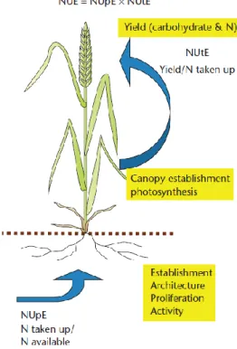
Now we can define Nitrogen Use Efficiency and their different parts. NUE is usually defined as the yield of grain relative to the amount of nitrogen available to the crop from all sources, including fertiliser, mineralisation in the soil and atmospheric deposition. NUE is the product of two main terms: nitrogen uptake efficiency (NUpE) and nitrogen utilisation efficiency (NUtE)(Moll et al., 1982) (Fig. 2 )

When N is limiting is necessary to optimize N-uptake from the dilute solution. Nitrogen uptake efficiency (NUpE) may be defined as the amount of N taken up by the crop as a fraction of the amount available to the crop from all sources. This is a root related trait and reflects the efficiency of root structure and function in capturing applied nutrients and nutrients within the soil.

When N-supply is such that the existing yield potential is reached, the only way of increasing production is to improve the efficiency with which N is used in metabolism (Lawlor, 2001). Nitrogen utilisation efficiency (NUtE) for grain is defined as grain yield divided by the amount of N taken up. Physiologically this is due to the photosynthetic efficiency of the canopy and the ability to produce grain yield as a function of the photosynthate fixed (Hawkesford, 2013). In this work we will work with NUpE and its variation in function of the N fertiliser applied and the cultivar. So we will speak more about this trait ahead.

1.4 Wheat nitrogen uptake and assimilation

To understand the parameters described before is essential to comprehend the crop N cycle better.

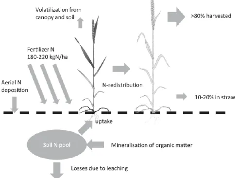
As in every ecosystem, in an intensive wheat system we have inputs and outputs of nitrogen connected by intermediate fluxes. The Figure 3 shows the major inputs, outputs and intermediate fluxes.

Figure 2. Illustration of nutrient use efficiency parameters exemplified by NUE in wheat. Key process contributing to the NUE trait: nitrogen uptake efficiency, NUpE; nitrogen utilisation efficiency, NUtE. Modified from Hawkesford (2011)

(11)

11

In a highly productive intensive wheat system the major input are from fertilizers, this account for 180-200 kg ha-1 as average in UK. Also is important the N provided by mineralization of organic matter, which is highly variable and mainly by factors like temperature, humidity, pH and aeration of the soil. Finally, additional N for the crop is provided by aerial deposition, wet or dry deposition. Goulding et al. (1998) showed in Broadbalk at Rothamsted, UK, that the wet deposition was 4 and 5 kg N ha-1 yr-1 of nitrate and ammonium respectively and a total deposition of all measured N species, wet and dry, to winter cereals of 45 kg N ha-1 yr-1, 79% as dry deposition. Of this total,5% is leached, 12% is denitrified, 30% immobilized in the soil organic matter and 53% taken off in the crop.

The first step is the uptake of this nitrogen in the soil by the roots. In wheat, most N is absorbed as nitrate (NO3-) but also as ammonium (NH4+) and organic-N in form of amino acids. The uptake of N depends on the concentration of N in the soil solution, on the volume of soil exploited by roots and on the efficiency of roots in absorbing this N (Lawlor, 2001). Therefore a high efficient N uptake requires a good root function both, in terms of architecture and activity. This will allow the uptake of N efficiently at a wide range of external concentrations (Hawkesford, 2011).

Transporters are involved within the plant to optimize translocation or storage of N, in roots, shoots and storage organs. They operate with high affinities for their substrates and are often under strong metabolic control to avoid imbalances of nutrient accumulation and to optimize uptake with growth rates (Hawkesford, 2011). Two families of NO3 -transporters have been characterized, the low affinity type and the high affinity type, the use of one or another depends of the NO3- concentration in the soil (Daniel-Vedele et al., 1998).

Figure 3. Idealized major fluxes of N in a high yielding wheat crop. Width of arrow is a qualitative indication of size of flux. From Hawkesford, (2013).

(12)

12

Once the NO3- is within the plant this has to be reduced to NH4+ by nitrate and nitrite reductase using electrons from photosynthetic electron transport or respiration, which in wheat occur more in leaves than in roots. This NH4+ reduced is converted by the GS/GOGAT enzyme reaction, and then incorporated in ‘carbon-skeletons’, to produce glutamine and asparagine, two compounds for N transport and storage. Once assimilated into glutamine and asparagine, N is incorporated into other amino acids via transamination reactions.

Assimilation of nitrogen in plants requires reducing power, ATP and C-skeletons. Reducing power and ATP can be delivered by photosynthesis or by glycolysis and respiration. C-skeletons for the GS/GOGAT reaction are generated also by photosynthesis (Azcón-Bieto y Talón, 2008). So, there is close interaction in the very earliest phases of N and C metabolism, both using the light energy, with some 10% of the electron flux in photosynthesizing leaves used in NO3- reduction (Lawlor, 2001).

NO3- reduction and the GS/GOGAT cycle are highly regulated by several signals, positively by NO3- concentration, light, C-skeletons, high C/N ratio…, and negatively mainly by high levels of N reduced (NH4+, amino acids…).

1.5 Nitrogen movement in wheat: Anthesis as key moment

In wheat, and in other plants, the plant life cycle can be roughly divided into two main phases with regard to N management.

During the pre-anthesis phase of growth, absorbed nitrate and ammonium are assimilated by the crop and used to build up the photosynthetic tissues containing large quantities of photosynthetic proteins, a prerequisite for yield generation, and the structural proteins in supporting tissues and vascular connections of the shoot system (Pask et al., 2012). Notably, the enzyme Rubisco (ribulose 1,5-bisphosphate carboxylase) alone can represent up to 50% of the total soluble leaf protein content in C3 species (Mae et al., 1983). This formation of leaves, photosynthetic tissue, and tillers, structural tissue, during the early growth will determine the later capacity for grain formation and assimilate production to fill them.

After anthesis and during grain filling, any further N taken up is likely to be allocated directly to the grain. However, much of the grain N will be from re-distribution from the canopy, thus ensuring an overall optimal usage of N taken up during the pre-anthesis phase (Hawkesford, 2013). So, pre-anthesis stored nitrogen in wheat is important because grain filling greatly depends on the remobilization of pre-anthesis nitrogen.

The contribution of leaf N remobilization to wheat grain N content is cultivar dependent, varying from 50 to 90 % (Masclaux et al., 2001). This remobilization of N depends on both environmental and genotypic factors. Environmental factors include N fertilization (delays onset of senescence and increases amount of N for remobilization), disease pressure, drought conditions (both enhancing senescence and decreasing NUE) (Barbottin et al.,

(13)

13

2005) and limited nitrate supplies (enhancing N remobilization in Arabidopsis) (Lemaître et al., 2008).

As conclusion of this part, we can state that nitrogen uptake is one of the most important factors in nitrogen nutrition. A high Nitrogen Uptake Efficiency implies that the plant can uptake N more efficiently from the soil and allocate most of it into the grain. Such plants would minimize loss of N from the soil and make more economic use of absorbed N. On the other hand, anthesis is a key moment in nitrogen nutrition, grain N content in wheat depends greatly on uptake of soil N prior to flowering. This N uptake prior to anthesis and stored in vegetative tissues is remobilized after anthesis in the grain.

1.6 Grain yield estimation using remote sensing methods

Estimation of cereal-crop yield is considered a priority in most research programs (Steinmetz et al., 1990) due to the relevance of food grain to world agricultural production. Non-destructive, real-time and accurate prediction of crop yield over large areas is critical for the formulation of national food policy, price control, and foreign grain trade (Jiang et al., 1999). Grain quality has received extensive interest from the government, enterprises, and consumers because of its increasing demand in recent years. Crop monitoring and yield forecasting can be done with models that range from statistical to mechanistic with a high number of input variables. However, under nonoptimal growing conditions, estimates of crop growth and yield using crop growth models often are inaccurate (Clevers, 1997). Remote sensing has been used for agricultural monitoring for more than three decades. Due to their timely and repetitive coverage, the remote sensing data have been recognized as a valuable tool for yield forecasting (Becker-Reshef et al. 2010). Inside remote sensing, Spectral reflectance provide information that may be used to determine a wide range of parameters, these may include an in-season estimation of grain yield (Aparicio et al,. 2000). As soon as 1980 Tucker et al. used ground-based spectral radiometers to identify the relationship between, the most used spectral reflectance index, normalized difference vegetation index (NDVI) and crop yield. Final grain yields were found to be highly correlated with NDVI.

Spectral reflectance of a crop canopy is obtained from measurements of reflected radiation. The ability to detect reflected radiation is derived from the fact that when a single light wave collides with a material it is restricted to three physical processes. It can be reflected from the surface, absorbed by the object, or transmitted through the object (Reynolds et al., 2012). Spectral reflectance from leaves at different wavelengths gives a unique spectral signature as it is influenced by the optical properties of the plant. Pigments in leaves absorb light strongly in the photosynthetically active radiation (PAR) region of the electromagnetic spectrum, but not in the NIR (750 nm–2500 nm) region (Knipling, 1970). This generates an absorption contrast between these two spectral regions, which can be

(14)

14

represented by various indices (Reynolds et al., 2012). This gap between the two regions can be affected if the plant is suffering a stress, such as N stress, and this response to stress can be measured using spectral reflectance indices.

Spectral reflectance indices are numerical indicators that use either specific wavelengths, or bands of the electromagnetic spectrum, to quantitatively relate changes in reflectance spectra to changes in physiological variables. Indices have the advantage of summarizing a large amount of information into a few numerical values, which may be evaluated simultaneously in each sample. In this context, the spectral reflectance indices have the potential to provide a non-destructive and fast in season estimate of grain yield.

(15)

Objectives David Soba Hidalgo

15 2.Objectives

This study had two main objectives. These objectives are:

a) To investigate the variability of Nitrogen Uptake Efficiency (NUpE) and other agronomic traits among a wide range of winter wheat genotypes and N levels.

b) Evaluate a broad range of spectral reflectance indices as potential screening tools to predict grain yield in winter wheat.

Specifics objectives of b) section are:

i) To evaluate the correlation of existing spectral reflectance indices with yield of winter wheat genotypes under different nitrogen levels.

ii) To determine the best growth stage to apply the spectral reflectance tools.

iii) To identify the most appropriate indices and make a model to predict wheat yield with them.

(16)

Materials and Methods David Soba Hidalgo

16 3. Materials and Methods

3.1 Site

A two year (2013-2014 and 2014-2015) field trail was conducted at Rothamsted Research (Harpenden, southern UK). The soil is a well-drained, flinty silt clay loam (25% clay) overlying clay with flints (50% clay). This soil is designate as “Aquic paleudalf” in the USDA system and “Chromic Luvisol” in the FAO system.

3.2 Weather conditions

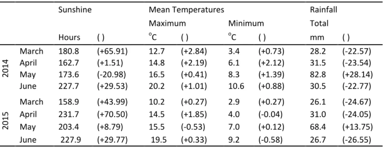
Weather data from tillering to anthesis in 2014 and 2015 in comparison with the 30 year mean values (1981-2010) are shown in Table 1. In 2014, sunshine and minimum and maximum temperatures were higher than normal, whereas precipitation was lower. So, this particular trend of the growing season (sunny and warm) was the principal cause of the advance in the anthesis data and the relative good yield. In 2015, sunshine was higher than normal, whereas precipitation was lower. Maximum and minimum temperatures were normal between tillering and anthesis.

Table 1. Monthly sunshine, temperatures and rainfall from tillering to anthesis at Rothamsted in 2014 and 2015. 30 year averages (1981-2010) are shown in brackets.

Sunshine Mean Temperatures Rainfall

Maximum Minimum Total

Hours ( ) oC ( ) oC ( ) mm ( ) 2014 March 180.8 (+65.91) 12.7 (+2.84) 3.4 (+0.73) 28.2 (-22.57) April 162.7 (+1.51) 14.8 (+2.19) 6.1 (+2.12) 31.5 (-23.54) May 173.6 (-20.98) 16.5 (+0.41) 8.3 (+1.39) 82.8 (+28.14) June 227.7 (+29.53) 20.2 (+1.01) 10.6 (+0.88) 30.5 (-22.77) 2015 March 158.9 (+43.99) 10.2 (+0.27) 2.9 (+0.27) 26.1 (-24.67) April 231.7 (+70.50) 14.5 (+1.85) 4.0 (-0.04) 31.0 (-24.05) May 203.4 (+8.79) 15.5 (-0.53) 7.0 (+0.12) 68.4 (+13.75) June 227.9 (+29.77) 19.5 (+0.33) 9.2 (-0.58) 26.7 (-26.55)

3.3 Soil N-min measurements

Soil cores were taken to 90 cm depth, before fertilizer was applied, for the analysis of mineral-N (NO3-N and NH4-N). The cores were taken with a ‘Hydro Soil Sampler’ fitted with a 3 cm diameter semi-cylindrical auger. Duplicate cores were taken from random positions across the field.

The cores were split into three depth sections, 0–30, 30–60 and 60–90cm and the mineral-N extracted by shaking 40 g of fresh soil with 100 ml of 2M KCl for 2 h. The slurry was allowed to settle for 30 min and then filtered. The solution was analysed for nitrate-N and ammonium-N with a ‘Skalar San Plus Analyser’. Concentrations in units of ppm in the

(17)

17

extracted solution were converted to field units of kg-N/ha by assuming a standard value of 1.5 g/cm3 for soil bulk density

Soils samples were found to have 24.65 kg ha-1 (2013) and 36.50 kg ha-1 (2014) mineral N (NO3-N + NH4-N) in the upper 90 cm profile (Table 2).

Table 2. Soil nitrate-N and ammonium-N contents (kg ha-1) at sowing within 0-30, 30-60, 60-90 cm soil depth in 2013-14 and 2014-15 growing seasons.

Year N Soil depth (cm) Total

0-30 30-60 60-90 NO3+NH4 2014 Nitrate-N 3.48 3.08 2.83 Amonium-N 8.39 4.82 2.05 24.65 2015 Nitrate-N 8.61 3.91 1.88 Amonium-N 11.98 7.64 3.48 36.50 3.4 Varieties

The experiment was conducted with 25 wheat varieties in 2013-2014 and with 25 wheat varieties in 2014-2015. Results presented here are from 23 varieties common to both years, two varieties were different each year.

Table 3. Wheat varieties common to both years, years of release, country (GBR-Great Britain, FRA-France, NDL-Nederland) and parents.

Variety Code Listed Country Parents

Avalon AV 1980 GBR Maris-Bilbo x Maris Plougham Bonham BO 2013 GBR Cordiale x postland

Cadenza CA 1992 GBR Tonic x Axona Claire CL 1999 GBR Flame x Wasp Cocoon CC 2010 GBR Wizard x Xi-19 Conqueror CN 2009 GBR Robigus x Equinox

Cordiale CO 2007 GBR (Reaper x Cadenza) x Malacca Crusoe CR 2011 GBR Cordiale x Gulliver

Evoke EV 2013 GBR Cordiale x Timaru

Gallant GA 2010 GBR (Malacca x Charger) x Xi-19 Hereford HF 2007 DNK Solist x Deben

Hereward HE 1989 GBR Normant x Disponent Istabraq IS 2004 GBR Consont x Claire

Malacca MA 1997 GBR (Riband x Rendezvous) x Apostle Maris Widgeon MW 1964 GBR Holfast x Capelle-Desprez Mercia ME 1984 GBR (Talent x Virtue) x Flanders Paragon PA 1998 GBR Csw-1724-19-5-68 x (Tonic x Axona) Riband RI 1987 GBR Norman x TW-275

Robigus RO 2005 GBR Z836 x 1366

Stigg ST 2010 GBR (Biscay x LW-96-2939) x Tanker Solstice SL 1987 FRA IENA x HN-35

Soissons SS 2002 NDL Vivant x Rialto

(18)

18

(Table 3). The varieties were representative cultivars in UK in recent years. The old variety Maris Widgeon were chosen to see how it would perform at low N level compared with modern cultivars. Maris Widgeon was registered in 1964 at the time when chemical fertilizers were not commonly used and it could be assumed that it would do well at low N level. There was also one spring variety (Paragon).

3.5 Nitrogen regimes

Nitrogen fertilizer, as ammonium nitrate prills, was applied at four rates of 0, 100, 200 and 350 kg-N ha-1, hereafter labelled as N1, N2, N3, and N4, respectively. The fertilizer was applied as a top-dressing in a 3-way split in March (nominally GS 24), April (GS 31) and May (GS 32) (Table 4).

Table 4. Nitrogen fertilizer rates and splits (kg-N/ha).

Treatment Total March (GS 24) April (GS 31) May (GS 32)

N1 0

N2 100 50 50

N3 200 50 100 50

N4 350 50 250 50

3.6 Experimental design

In 2014 and 2015, 25 varieties were grown at 4 N-rates. The experimental design was a randomised complete block design with three replications and a factorial combination of four N levels (300 plots). Plots were 9 m long and 3 m width, were sown at a density of 350 grains m-2. The experimental design layout can be found in the APPENDIX I.

3.7 Husbandry

The trials were conducted in different fields at Rothamsted over two seasons, 2014 (Great Harpenden field), 2015 (Bones close field) (harvest years are shown). All crops were first wheat to avoid effects from the root disease ‘take all’ which is prevalent in continuous wheat crops in the UK. The crop before were given modest amounts of N-fertilizer which ensured relatively low residual soil- N-min levels for the following wheat. All crops were autumn-sown (including the spring variety) on October 2nd in 2014 and on October 1st in 2015. Seeds were precision-drilled at a rate of 350 seeds m-2 in 12.5 cm rows in plots measuring 3 m by 9 m. Available soil P, K and Mg was Index 2 on all fields which is non-limiting to yield (MAFF, 2000). Crops were top-dressed with potassium sulphate in March supplying sulphur at a rate of 20 kg-S ha-1. Crops were given growth regulator and protected against weeds, pests and diseases as required.

(19)

19 3.8 Crop measures

Anthesis dates were recorded when stamens were visible on 50% of the spikes. In this moment 1 m2 representative, avoiding border effect, of each plot was manually cut at ground level, the number of ears m-2, and the chlorophyll, using a SPAD meter, were measured. Then the samples were oven-dried at 80 ºC to a constant weight and the biomass dry weight (DM) at anthesis measured. Samples were ground by a rotor mill and a small portion was taken. Then the % of N in the shoots was measured. The N uptake (Nt) at anthesis was measured as the total above-ground N (dry biomass multiplied by % N in the shoots). Nitrogen Uptake Efficiency (NUpE) was calculated as total above-ground N content at anthesis/soil N supply (Nt/Ns). N supply (Ns) was the sum of N applied as fertilizer plus N mineral in the upper 90 cm soil profile.

3.9 Statistical analysis

To determine the significance of main effect of year, N level and genotype and interaction ANOVA for all measurements was performed using SPSS (22.0 for Windows). To demonstrate relationship between NUpE and related trait, linear regression and correlation analysis were used.

3.10 Grain Yield Prediction

3.10.1 Spectral reflectance measurements

To measure spectral reflectance, a spectro-radiometer was used, with a spectral range of 360nm–1000 nm. This continuous range encompasses the visual and near-infrared regions of the electromagnetic spectrum and is sufficient for measuring the wavelengths used for most canopy related indices. Reflected radiation from the canopy is received by a foreoptic lens, and relayed to the spectro-radiometer via a fiber-optic cable.

A white reference panel is used to calibrate the equipment at start each day. It should be Lambertian surfaces; these reflect incident radiation of all wavelengths equally in all directions, and are required to provide a reference for the calculation of reflectance units. To make the model, measurements, were taken approximately weekly from the end of April to leaf senescence (end of July). Measurements were made around midday. One spectral reflectance measurement was taken at each plot, being the average of fifteen scans. The reflectance spectrum was calculated in real time as the ratio between the reflected and the incident spectra on the canopy. Radiometric indices were calculated from spectral reflectance measurements.

To use the model during the next season, 2014-15, three measures around anthesis (12, 15 and 18 of June) were taken following the same steps before commented.

(20)

20 3.10.2 Spectral Reflectance Indices

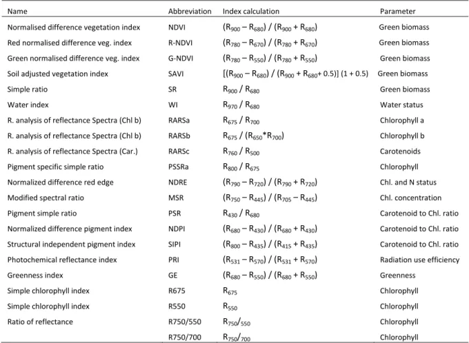
The spectral raw data were transformed into reflectance in each wavelength using a excel spreadsheet. With this data different spectral reflectance indices were calculated. In total, 21 spectral reflectance indices were used to assess the crop status. These indices were related, among others, with crop biomass, chlorophyll content, nitrogen status, ratio chlorophyll:carotenoids, water status, radiation use efficiency… (Table 5).

Spectral reflectance indices were calculated for each measurement along the vegetative cicle (12 times).

Table 5. Spectral reflectance indices used in this work.

Name Abbreviation Index calculation Parameter

Normalised difference vegetation index NDVI (R900 – R680) / (R900 + R680) Green biomass Red normalised difference veg. index R-NDVI (R780 – R670) / (R780 + R670) Green biomass Green normalised difference veg. index G-NDVI (R780 – R550) / (R780 + R550) Green biomass Soil adjusted vegetation index SAVI [(R900 – R680) / (R900 + R680+ 0.5)] (1 + 0.5) Green biomass

Simple ratio SR R900 / R680 Green biomass

Water index WI R970 / R680 Water status

R. analysis of reflectance Spectra (Chl b) RARSa R675 / R700 Chlorophyll a R. analysis of reflectance Spectra (Chl b) RARSb R675 / (R650*R700) Chlorophyll b R. analysis of reflectance Spectra (Car.) RARSc R760 / R500 Carotenoids Pigment specific simple ratio PSSRa R800 / R675 Chlorophyll Normalized difference red edge NDRE (R790 – R720) / (R790 + R720) Chl. and N status Modified spectral ratio MSR (R750 – R445) / (R705 – R445) Chl. concentration Pigment simple ratio PSR R430 / R680 Carotenoid to Chl. ratio Normalized difference pigment index NDPI (R680 – R430) / (R680 + R430) Carotenoid to Chl. ratio Structural independent pigment index SIPI (R800 – R435) / (R415 + R435) Carotenoid to Chl. ratio Photochemical reflectance index PRI (R531 – R570) / (R531 + R570) Radiation use efficiency Greenness index GE (R680 – R550) / (R680 + R550) Greenness

Simple chlorophyll index R675 R675 Chlorophyll

Simple chlorophyll index R550 R550 Chlorophyll

Ratio of reflectance R750/550 R750/550 Chlorophyll

R750/700 R750/700 Chlorophyll

3.10.3 Model construction and validation

Simple linear regressions were developed between grain yield as dependant variable and spectral reflectance indices as independent variable for the year 2013/14. However, due to the fact that the crop covers increase in a logarithm way with increasing N fertilizer, the reflectance of radiation by the crop is saturate with high inputs. This fact can be seen if we represent the most popular spectral reflectance index (NDVI) against Leaf Area Index (LAI). We can see, as is reported in other studies (Aparicio et al., 2000), that NDVI is saturated when the LAI is higher than 3. This fact is also observed in other indices like SAVI, PRI, GI,

(21)

21

SIPI, WI… and make impossible a linear relation between the four treatments. However is possible a linear relation if we exclude the no nitrogen treatment (N1) and we work with N2, N3 and N4. Therefore, to linear regressions, only the N-treatments N2, N3 and N4 were used.

These simple linear regression models allowed to see which indices and which crop stage were the better to predict grain yield. The five better related indices and the best related moment were chose to do a model. The weight of each spectral reflectance index was optimice to get the best coefficient of determination and RMSE.

Evaluation is an important step of model verification which determines how closely a model represents actual conditions. Following statistical indicators were employed to compare the estimate and observed data.

The coefficient of determination (r2) represents the percent of data that is the closest to the line of best fit. r2 equal to 1.0 indicates perfect fit and lesser values indicating less agreement of data.

Where RMSE is absolute root mean square error, nRMSE is normalized mean square error expressed in %, Pi is the predicted value, Oi is the observed value, N is the number of observations and M is the mean of observed value. RMSE close to zero indicates better model performance. nRMSE is a measure (%) of the relative difference of estimated versus observed data. The prediction is considered excellent with the nRMSE <10 %, good if 10–20 %, fair if 20–30 %, poor if >30 % (Jamieson et al. 1991).

(22)

Results David Soba Hidalgo

22 4. Results

4.1 Genetic differences for nitrogen uptake efficiency

Analysis of variance showed significant differences among genotypes for all traits, except for shoot N yield and N uptake efficiency (Table 6).

Although differences between both years were generally significant, results were consistent, as the year x genotype x N level interaction was never significant. Results will then be presented averaged over the 2 years (Table 7). Nevertheless, results of biomass, shoot N concentration, shoot N yield and NUpE were also presented for each year (Table 8). Differences between the N levels and the different traits were always significant. The G x N interaction was significant for height and chlorophyll. In all the traits the greatest source of variation was the amount of nitrogen fertilizer applied followed, generally, by year and genotype.

Only chlorophyll, height and the number of ears m-2 showed significant varietal differences at all N-rates.

Biomass

Biomass, above ground dry matter, was significantly higher in the 2015 than in 2014, except for the treatment N4 (Table 6, P<0.01). N was the greatest source of variation (F = 1032). The application of N fertilizer increased biomass of all genotypes, from 4.67 t ha-1 on average at lowest N fertilizer plots to 13.43 t ha-1 at highest N fertilizer plots (Table 7). Biomass was also significantly different between genotypes. For example, at lowest N1, biomass ranged between 3.9 and 5.3 t ha-1 and at N2 from 9.26 to 15.62 t ha-1. Only the interaction between nitrogen and year was significant.

Shoot N concentration

Significant variation was shown for shoot N concentration among nitrogen, genotype, year and nitrogen x year interaction. The application of N fertilizer increased %N of all genotypes. All the genotypes had the lower value at N1. Genotype and year was also significant, %N was 10% higher in 2014 than in 2015. The varieties Riband, Mercia, Malacca and Avalon had the highest mean concentrations (around 1.2 %) and Soissons the lowest (0.99%).

Shoot N yield

Shoot N yield has been defined as biomass x shoot %N, so was highly influenced by this two traits. The ANOVA revealed significant variation among N level, year and the interaction nitrogen and year. The relation between nitrogen and the shoot N yield was linear with the minimum at N1 (33 kgN ha-1) and the maximum at N4 (227 kgN ha-1). The varieties Crusoe, Cocoon and Stigg had the highest mean over all N levels (~135 kgN ha-1)

(23)

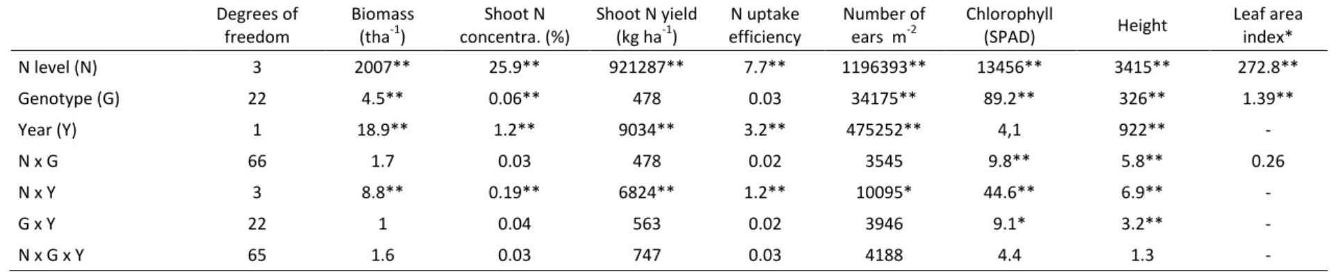
Table 6. Analysis of variance (mean squares) for biomass (t ha-1), Shoot N concentration (%), Shoot N yield (kg ha-1), Nitrogen Uptake Efficiency (NUpE), ears (nº m-2), chlorophyll (SPAD), plant height (cm) and Leaf Area Index (m2 m-2) at anthesis; mean values for N rates and years. *Only 2014.

*, significant at P<0.05; **significant at P<0.01 Degrees of freedom Biomass (tha-1) Shoot N concentra. (%) Shoot N yield (kg ha-1) N uptake efficiency Number of ears m-2 Chlorophyll (SPAD) Height Leaf area index* N level (N) 3 2007** 25.9** 921287** 7.7** 1196393** 13456** 3415** 272.8** Genotype (G) 22 4.5** 0.06** 478 0.03 34175** 89.2** 326** 1.39** Year (Y) 1 18.9** 1.2** 9034** 3.2** 475252** 4,1 922** - N x G 66 1.7 0.03 478 0.02 3545 9.8** 5.8** 0.26 N x Y 3 8.8** 0.19** 6824** 1.2** 10095* 44.6** 6.9** - G x Y 22 1 0.04 563 0.02 3946 9.1* 3.2** - N x G x Y 65 1.6 0.03 747 0.03 4188 4.4 1.3 -

(24)

24

and Soissons had the lowest mean (112 kgN ha-1). At N3 (200 kgN applied ha-1) which is the common amount of N fertilizer applied in developed countries, Paragon, Bonham and Conqueror had the highest amount of N uptake and Soissons the lowest. The varietal range of apparent fertilizer recoveries at N3 was 53-71%.

Nitrogen Uptake Efficiency

Nitrogen Uptake Efficiency (NUpE) was calculated as total nitrogen uptake above ground/N in the soil and applied. As for N Uptake significant variation was revealed for NUpE among N level, year and the interaction nitrogen and year. In this case although nitrogen is again the greatest source of variation, year is also very important (almost the same than nitrogen). NUpE was 25% higher in 2014 than in 2015 and the biggest difference can be saw at low N level (N1) where the effect of the soil-N-min is more important in NUpE (Table 8). In this case, in contrast to Shoot N yield, the relation between nitrogen and the NUpE was logarithmic with the maximum at N1 (1.12) and the minimum at N4 (0.60). As commented with the shoot N yield, at N3 Paragon, Bonham and Conqueror had the highest amount of N uptake efficiency and Soissons the lowest.

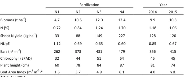
Table 7. Biomass (t ha-1), Shoot N concentration (N (%)), Shoot N yield (kg ha-1), Nitrogen Uptake Efficiency (NUpE), ears (nº m-2), chlorophyll (SPAD), plant height (cm) and Leaf Area Index (m2 m-2) at anthesis; mean values for N rates and years.

*Only for 2014 Chlorophyll

Significant variation was revealed for chlorophyll among nitrogen, genotype, and the interaction between nitrogen and genotype and between nitrogen and year. Nitrogen was the greatest source of variation. The mean value of chlorophyll, measure using Chlorophyll meter, at N1 was 58% of the value at N4. The highest values of chlorophyll were reached by Cadenza, Maris Widgeon showed the lowest values. Computing the ecovalence showed that three genotypes, Mercia, Riband and Istabraq, were responsible for about one-third of the G x N interaction. In this case the differences between the two years were not significant. Fertilization Year N1 N2 N3 N4 2014 2015 Biomass (t ha-1) 4.7 10.5 12.0 13.4 9.9 10.3 N (%) 0.72 0.84 1.24 1.70 1.18 1.06 Shoot N yield (kg ha-1) 33 88 149 227 128 120 NUpE 1.12 0.69 0.65 0.60 0.85 0.67 Ears (nº m-2) 262 373 431 479 356 415 Chlorophyll (SPAD) 32 44 51 54 45 45 Plant height (cm) 60 78 84 87 81 74

(25)

25 Ears m-2

The ANOVA for Ears m-2 revealed significant variation among N level, genotype, year and the interaction nitrogen and year. Again nitrogen was the greatest source of variation (F = 330) but year was also greater (F = 131). The relation between nitrogen and the number of ears m-2 was logarithmic with the minimum number at N1 (262 ears m-2) and the maximum at N4 (479 ears m-2). The number of ears was 17% higher in the 2014/15 than in 2013/14 growing season.

Leaf Area Index (LAI)

LAI was measured, at anthesis, only in the 2013/14 growing season. Significant variation was revealed for LAI among nitrogen and genotype. The relation between nitrogen and LAI was linear with the minimum value at N1 (1.5 m2m-2) and the maximum at N4 (6.1 m2m-2) for all genotypes. G x N interaction was not significant.

Height

Significant variation was shown for height among genotype, nitrogen, year and all their interactions. Nitrogen was the greatest source of variation but year and genotype were also important. The mean value of height at N1 was 60 cm and 87 cm at N4. Plant height was significantly higher in the 2014 than in 2015 growing season in all the treatments. The difference between the tallest variety (Maris Widgeon) and the shortest (Cordiale) were 42 cm. The tallest variety Maris Widgeon was responsible for most of the G x N interaction (38%), additionally; Paragon represented 10% of the G x N interaction.

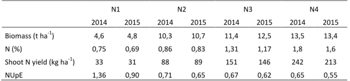
Table 8. Biomass (t ha-1), Shoot N concentration (N (%)), Shoot N yield (kg ha-1) and Nitrogen Uptake Efficiency (NUpE) at anthesis; mean values for N levels for 2014 and 2015 years.

N1 N2 N3 N4 2014 2015 2014 2015 2014 2015 2014 2015 Biomass (t ha-1) 4,6 4,8 10,3 10,7 11,4 12,5 13,5 13,4 N (%) 0,75 0,69 0,86 0,83 1,31 1,17 1,8 1,6 Shoot N yield (kg ha-1) 33 31 88 89 151 146 242 213 NUpE 1,36 0,90 0,71 0,65 0,67 0,62 0,65 0,55

(26)

26

Figure 4. Boxplots for Biomass (t ha-1), Shoot N concentration (N (%)), Shoot N yield (kg ha-1), Nitrogen Uptake Efficiency (NUpE), chlorophyll (SPAD), plant height (cm) depending on the N treatment.

(27)

27

4. 2 Spectral reflectance indices as tools for predicting wheat grain yield 4.2.1 Spectral signatures

Using all the lectures from the spectro-radiometer is possible to make a complete reflectance spectrum in the visible and part of the NIR region. The overall mean of spectral reflectance of wheat crop (treatment 200 kg N ha-1) at different stages is plotted in figure 5. It may be seen that the spectral reflectance characteristics are different at different stages. Changes in canopy structure and pigments throughout the development stages were translated into changes in the spectral signature. During jointing stage the canopy was not fully developed and soil contribution to the canopy reflectance was large, although the spectral signature showed characteristic features of green vegetation (lower reflectance in the red region and bigger in the NIR region). As the canopy developed, reflectance in the NIR region increased reaching the maximum at anthesis. As the crop growth progressed further, during the grain filling, the remobilization of the N content in the photosynthetic pigments in the leaves to the grain affected the canopy reflectance and the reflectance contrast between red and NIR regions started to reduce. At maturity, vegetation was senescence and the spectral signature showed a steady linear increase across the red region.

Figure 5. Spectral reflectance characteristics of the wheat canopy (treatment N3) at different phonological stages (n=75)

4.2.2 Spectral reflectance at anthesis as influence by nitrogen

The reflectance spectra at anthesis for the four N treatments are shown in the figure 6. The difference between the four treatments is visible. As we will see later with the spectral

0,0 0,1 0,2 0,3 0,4 0,5 0,6 360 440 520 600 680 760 840 920 1000 Re fl ec tan ce Wavelength (nm) Jointing Booting Anthesis Grain filling Maturity

(28)

28

reflectance indices, there are a big different between the no nitrogen treatment and the other 3 treatments.

Different reflectance was measured in each region between treatments. Plant stress (or leaf senescence) typically results in lower chlorophyll concentrations that allow expression of accessory leaf pigments such as carotenes and xanthophylls. This has the effect of broadening the green reflectance peak (normally located near 550 nm) towards longer wavelengths, increasing visible reflectance, and causing the tissues to appear chlorotic (Pinter et al., 2003), as we can see in N1 treatment in figure 6. At the same time, with N stress, NIR reflectance decreases. With no nitrogen the crop surface reflects more radiation in the visible region than in the others treatment but less in the NIR region. This means that the leap between the visible and the NIR regions is higher with increasing nitrogen fertilization. However this increase is not linear, since, as the nitrogen fertilizer increased the difference is less marked getting an asymptote. This abrupt transition or “red edge”, in the case of senescent vegetation, may disappear entirely (Figure 5).

Figure 6. Reflectance spectra, at anthesis, of the four N treatments. (n = 75) 4.2.3 Nitrogen effects on Normalized difference vegetation index (NDVI)

The NDVI, as indicator of crop vigour status, as influenced by nitrogen is shown in figure 7. NDVI values varied from 0.20 to 0.95. NDVI increased to its maximum values at booting (225 days after sowing (DAS)) maintaining its values until anthesis (252 DAS), before in N1. After anthesis the NDVI value decreased abruptly, reaching its minimum at maturity when the leaves were completely senescence. However, in the treatment N1, the maximum value of NDVI was reached at heading (240 DAS) and from this moment the NDVI value decreased slowly until maturity. Among all the N treatments, NDVI was maximum in the treatment N4 and minimum in the treatment N1. The differences between the treatments N2, N3 and N4 were small, and bigger between these three treatments and treatment N1.

0,0 0,1 0,2 0,3 0,4 0,5 0,6 400 500 600 700 800 900 1000 R e fl e ctan ce Wavelength (nm) N1 N2 N3 N4

(29)

29

Figure 7. Temporal variation of NDVI under different nitrogen treatments. (n = 75)

4.2.4 Relations between Spectral reflectance indices at different crop stages and grain yield The correlation coefficients of the linear regressions between the grain yield measured at harvest and the 21 spectral reflectance indices used in this work are shown in table 9. This table include different data from the end of April to leaf senescence (end of July) and the treatment N1 (no nitrogen) was not included in the simple linear regressions.

Figure 8. Relationships between spectral reflectance indices measured at anthesis and grain yield. Each point represent each plot of the experiment (variety Maris Widgeon is not take into account) (n = 288). See table 5

for index definitions.

0 0,1 0,2 0,3 0,4 0,5 0,6 0,7 0,8 0,9 1 200 210 220 230 240 250 260 270 280 290 300 310 N D VI

Days after sowing (DAS)

N1 N2 N3 N4

(30)

30

N1 treatment was no taken into account because, as we can see in figure 8, a curvilinear response between spectral reflectance indices and grain yield made difficult comparisons between the different indices and the grain yield using the four treatments. However if the no nitrogen treatment was excluded a linear relation could be obtained.

NDRE, related with the nitrogen status of the crop, and MSR, related with the chlorophyll concentration, were the best indices to predict the grain yield, not only at anthesis but also before and after this moment. G-NDVI, used to measure the chlorophyll and biomass, and PRI, related with radiation use efficiency, were also other indices well related with the grain prediction at anthesis. The WI, related with the water status of the crop, is well related with grain yield but mainly after anthesis. Chlorophyll b (RARSa) content is also well related with grain yield. As we can see in figure 9 and in table 9, around anthesis was the moment with higher correlations between the five selected spectral indices and grain yield so this moment was chose to make the model.

Figure 9. Coefficients of determination (r2) of the relationship between wheat grain yield at maturity and the spectral reflectance indices and the days from the first spectral reflectance measure.

(31)

Table 9. Coefficients of determination (r2) of the relationship across genotypes between wheat grain yield at maturity and the spectral reflectance indices at different growth stages in treatments N2, N3 and N4 in WW1416 experiment at Rothamsted, UK (n = 216).

NDVI R-NDVI

G-NDVI SAVI SR WI RARSa RARSb RARSc PSSRa NDRE MSR PSR SIPI NDPI PRI GI R675 R550 R750/R550 R750/R700 28/04/2014 0.19 0.19 0.44 0.13 0.25 0.23 0.01 0.42 0.28 0.26 0.57 0.53 0.18 0.13 0.18 0.21 0.02 0.35 0.13 0.24 0.02 06/05/2014 0.25 0.26 0.58 0.06 0.36 0.29 0.00 0.72 0.26 0.38 0.73 0.56 0.36 0.02 0.36 0.49 0.02 0.54 0.15 0.44 0.03 14/05/2014 0.28 0.28 0.54 0.10 0.37 0.27 0.00 0.56 0.23 0.37 0.68 0.73 0.44 0.26 0.42 0.53 0.03 0.41 0.10 0.49 0.03 29/05/2014 0.65 0.65 0.76 0.03 0.62 0.33 0.01 0.64 0.41 0.62 0.81 0.81 0.55 0.46 0.53 0.70 0.07 0.54 0.10 0.55 0.05 06/06/2014 0.57 0.56 0.72 0.46 0.49 0.45 0.04 0.50 0.30 0.48 0.81 0.80 0.58 0.55 0.58 0.73 0.01 0.38 0.04 0.63 0.00 Anthesis 0.63 0.63 0.77 0.55 0.62 0.60 0.00 0.64 0.40 0.62 0.85 0.85 0.65 0.61 0.63 0.76 0.14 0.51 0.51 0.71 0.77 13/06/2014 0.60 0.60 0.74 0.46 0.56 0.71 0.07 0.59 0.30 0.56 0.82 0.80 0.61 0.63 0.60 0.68 0.04 0.59 0.09 0.61 0.01 19/06/2014 0.56 0.56 0.69 0.42 0.56 0.79 0.02 0.68 0.39 0.56 0.74 0.69 0.47 0.51 0.47 0.52 0.10 0.65 0.16 0.49 0.07 24/06/2014 0.55 0.54 0.64 0.50 0.52 0.74 0.00 0.60 0.36 0.52 0.70 0.67 0.46 0.51 0.48 0.54 0.23 0.57 0.14 0.49 0.19 03/07/2014 0.58 0.58 0.63 0.56 0.51 0.62 0.27 0.49 0.45 0.51 0.67 0.57 0.47 0.52 0.50 0.57 0.45 0.50 0.18 0.54 0.45 16/07/2014 0.46 0.43 0.41 0.50 0.34 0.29 0.25 0.06 0.26 0.31 0.46 0.36 0.24 0.49 0.26 0.28 0.31 0.42 0.07 0.53 0.00 29/07/2014 0.06 0.00 0.01 0.35 0.05 0.02 0.01 0.07 0.00 0.00 0.02 0.00 0.05 0.00 0.06 0.02 0.02 0.10 0.10 0.05 0.03

NDVI. Normalised difference vegetation index; R-NDVI. Red normalised difference vegetation index; G-NDVI. Green normalised difference vegetation index; SAVI. Soil adjusted vegetation index; SR. Simple ratio; WI. Water index; RARSa. Ratio analysis of reflectance spectra (Chla); RARSb. Ratio analysis of reflectance spectra (Chlb); RARSc. Ratio analysis of reflectance spectra (Carotenoids); PSSRa. Pigment specific simple ratio; NDRE. Normalised difference red edge; MSR. Modified spectral ratio; PSR. Pigment simple ratio; SIPI. Structural independent pigment index; PRI. Photochemical reflectance index; GE. Greenness index; R675. Simple chlorophyll index (high sensitivity); R550. Simple chlorophyll index (low sensitivity); R750/R550 and R750/R700. Ratio of reflectance.

(32)

32

So we can state that wheat grain yield, at maturity, is well related to N status of the crop, amount of chlorophyll and with canopy and radiation use efficiency (RUE) at anthesis. 4.2.5 Grain yield prediction model

In the light of the prior table, I have tried to make a model to predict the grain yield at maturity, with information obtained between two and three months in advance.

To do this, I have chosen five spectral reflectance indices well related, at anthesis, with grain yield at maturity. These are: Green normalised difference vegetation index (G-NDVI), Water index (WI), Normalised difference red edge (NDRE), Modified spectral ratio (MSR), Photochemical reflectance index (PRI). These indices are related with: crop N status (NDRE), chlorophyll content (MSR), chlorophyll and biomass (G-NDVI), Radiation use efficiency (PRI) and water status (WI). Table 10 shows the most important statatistic obtained from the models which, using these five spectral reflectance indices, predict grain yield.

Table 10. The most important statistics obtained from the simple regression models to estimate yields based in five spectral reflectance indices.

Model n Equation r2 RMSE (t ha-1) nRMSE (%)

G-NDVI 216 GY = 39.982*G-NDVI-20.966 0.77 0.928 8.0

WI 216 GY = 59.909*WI+60.088 0.60 1.213 10.4

NDRE 216 GY = 24.525*NDRE-2.0082 0.85 0.743 6.4

MSR 216 GY = 0.8224*MSR+4.7434 0.85 0.740 6.3

PRI 216 GY = 115.59*PRI+13.459 0.77 0.938 8.0

n: number of samples; r2: model coefficient of determination; RMSE: root mean square error; nRMSE: ratio between RMSE and yield. Data correspond to treatments N2, N3 and N4 at anthesis. Data from spectral measures taken on 10th of June.

Regression models developed between the grain yield of wheat and the spectral reflectance indices of the year 2013–14 showed that G-NDVI, WI, NDRE, MSR and PRI could account for 77, 60, 85, 85 and 77 % variation in the grain yield of wheat respectively (Table 10). Out of the five SRI based regression models, NDRE and MSR based models resulted in lowest RMSE (0.74 t ha-1) and lowest nRMSE (±6 %) compared to PRI and G-NDVI (RMSE=0.94 t/ha and nRMSE, 8 %) and WI (RMSE=1.21 t ha-1 and nRMSE, 10.4 %) based models.

To make a model, the number of data is very relevant. Therefore, I have chosen the three days near to anthesis. These days are: 6, 10 and 13 of June, in total 864 data (the variety Maris Widgeon has been deleted because this variety has high spectral reflectance indices (high LAI) but low grain yield, so can make the model inconsistent). Three days have been choosen instead one to try to eliminate exogenous factors that can affect remote observations such as view angle, row orientation, meteorological phenomena… The model was made with the linear equations between the five spectral reflectance indices before said and the grain harvested at maturity in these three days of June (Figure 10).

(33)

33

But, once the model was make both water status (WI) and biomass of the crop (G-NDVI) has a bad effect in the proposed model, thereafter the next model was proposed (Figure 11). It was calibrated to get the maximum coefficient of determination between the grain yield at maturity and the predicted grain at anthesis. The weight of each factor in the model is: N status (40%). chlorophyll (40%) and RUE (20%) (Table 11).

In this model the two main factors which have influenced in the model are the N status and the chlorophyll content in the canopy. These two factors are much related between them, approximately 75% of the plant´s N is contained in the chloroplasts (Lawlor, 1995). In a second place, the radiation use efficiency (RUE) with the 20% of the model weight. RUE is very closely linked with the chlorophyll concentration in the leave. So, the N status of the crop is a key factor in future grain yield.

Figure 10. Proposed model to predict grain yield at anthesis

(34)

34

Table 11. Predictive model of grain yield of wheat at anthesis (developed from 2013-14 data).

Parameter Stage Index Predictive equation r2 Weight Grain yield

(GY in t/ha) Anthesis

NDRE GY=24.454*NDRE - 2.0725 r2 = 0.96 (n=864) 40% MSR GY=0.8186*MSR + 4.6592 r2 = 0.94 (n=864) 40% PRI GY=111.16*PRI + 13.239 r2 = 0.94 (n=864) 20%

With these changes the graphic representation between the grain yield measure at maturity and the predicted grain by the model is shown in the figure 12 and table 11.

Figure 12. Relationship between in-season estimated grain yield (EY) and measured grain yield in WW1416 experiment at Rothamsted. UK (n=288)

Table 12. The most important statistics obtained from the predictive model of grain yield of wheat at anthesis (developed from 2013-14 data).

Treatment n Equation r2 RMSE (t ha-1) nRMSE (%)

N1 72 GY=1.0182x-0.7545 0,452 0,790 20,08 N2 72 GY=0.8021x+1.6965 0,424 0,660 7,01 N3 72 GY=0.6795x+3.8873 0,500 0,631 5,25 N4 72 GY=0.7995x+3.1029 0,463 0,915 6,75 N2, N3 & N4 216 GY=1.0844x-0.8703 0,858 0,746 6,40 All 288 GY=1.05x-0.46 0,969 0,758 7,80

n: number of samples; r2: model coefficient of determination; RMSE: root mean square error; nRMSE: ratio between RMSE and yield. Data from spectral measures taken on 10th of June.

y = 1.05x - 0.46 R² = 0,97 RMSE (t/ha) = 0.758 nRMSE (%) = 7.8 0 2 4 6 8 10 12 14 16 0 2 4 6 8 10 12 14 16 M e asu re d g rai n yi e ld , tn h a -1

(35)

35

As we can see in the prior table, the best correlation coefficient was obtained if the four treatments were taken into account. All the treatments (except N1) shown a normalized mean square error (nRMSE) <10% which can be considered an excellent prediction.

4.2.6 Prediction with the model

The grain yield prediction model was make using three different indices around anthesis and the harvest yields from 2013/14 data. To predict the 2014/15 grain yield at harvest, another three spectral reflectance measures were collected around anthesis (12, 15 and 18 of June) and the three indices (NDRE, MSR and PRI) were calculated and introduced in the model.

Table 13. Predicted grain yield at anthesis (3 different days) under different nitrogen treatments. N-treatment Predicted Grain Yield (t ha

-1

)

12/06/2015 15/06/2015 18/06/2015 Mean

N1 4.34a 4.49a 4.56a 4.47a

N2 8.54b 8.63b 8.72b 8.63b

N3 11.51c 11.80c 11.52c 11.61c

N4 12.85de 13.10e 12.72d 12.89de

Numbers followed by same letter are not significantly different at P=0.05.

The predictions for the three days are shown in table 13 and, graphically, in figure 13. As we can see the measurements in the three days were very similar and, except for the treatment N4, the data were not significantly different. The minimum yield predicted were in the treatment N1 (4.5 t ha-1) and reached its maximum in N4 (almost 13 t ha-1). The relation between predicted grain yield and N fertilizer applied was logarithmic with a high increase between N1 and N2 (figure 14).

(36)

36

Figure 14. Relationship between predicted grain yield and N fertilizer applied.

The predictions for each variety can be seen in table 14. As we can see in treatment N3 (200 kgN ha-1), which is the average N-application in UK and many developed countries, the highest values were coincidet with the high yielding varieties (Cocoon, Evoke, Hereford and Istabraq) while the lowest values predicted agree with low yielding varieties (Avalon, Mercia, Malacca, Soissons).

Table 14. Average predicted grain yield for the different varieties at different N-levels. Variety Predicted Grain Yield (t ha

-1 ) N1 N2 N3 N4 Avalon 3.96 8.21 11.31 12.44 Bonham 4.16 8.42 11.69 12.57 Cadenza 4.28 8.66 11.42 12.87 Cocoon 4.60 9.10 12.66 13.24 Claire 4.92 8.72 11.93 12.66 Conqueror 4.55 8.39 11.80 13.19 Cordiale 4.38 8.69 11.96 13.05 Crusoe 4.24 8.20 11.70 13.26 Evoke 4.54 8.87 12.09 14.13 Gallant 4.41 8.49 11.73 13.52 Hereward 4.83 8.76 11.68 12.89 Hereford 4.17 8.80 12.06 13.35 Istabraq 4.28 9.11 12.07 13.77 Malacca 4.32 8.18 10.62 12.34 Mercia 4.41 8.48 10.60 11.87 Paragon 4.36 8.50 11.28 11.86 Riband 4.11 8.56 11.17 12.88 Robigus 4.53 9.02 11.55 12.86 Solstice 4.97 8.80 11.96 13.31 Soissons 3.98 8.19 10.62 11.82 Stigg 4.85 9.04 11.68 13.10 Xi19 4.63 8.60 11.93 13.02 0 2 4 6 8 10 12 14 0 100 200 300 400 Pr e d ic te d Gr ai n Yi e ld (t /h a)

N fertilizer applied (kg/ha)

Mean Day 1 Day 2 Day 3

(37)

37 4.2.7 Validation of the model

As we can see in figure 15, where the relation between the grain yield predicted at anthesis and the observed grain yield at harvest is shown, the model can explain about the 96% of the variation in grain yield. The absolute root mean square error is about 1.5 and the normalized mean square error is less than 20%.

Figure 15. Relationship between in-season estimated grain yield (EY) and measured grain yield in WW1501 experiment at Rothamsted. UK (n=288)

The most important statistics obtained from the model are shown in table 15. The model applied for each N level can explain between 12 and 62 % of the variation in grain yield for each treatment. The nRMSE was in all cases between 10 and 20% which according with Jamieson et al. (1991) can be considered as good prediction.

Table 15. The most important statistics obtained from the calibration of the predictive model of grain yield of wheat at anthesis (developed from 2014-15 data).

Treatment n Equation r2 RMSE (t ha-1) nRMSE (%)

N1 72 GY=0.5918x+1.395 0.306 0.580 14.44

N2 72 GY=0.4465x+3.865 0.123 1.045 13.56

N3 72 GY=0.5868x+3.109 0.346 1.783 17.96

N4 72 GY=1.0896x+3.230 0.618 2.155 19.87

All 288 GY=0.8043x+0.567 0.962 1.523 18.75

n: number of samples; r2: model coefficient of determination; RMSE: root mean square error; nRMSE: ratio between RMSE and yield.

y = 0,8043x + 0,567 R² = 0,962 RMSE (t/ha) = 1.523 nRMSE (%) = 18.75 R² = 0,3055 R² = 0,1229 R² = 0,3456 R² = 0,6195 0 2 4 6 8 10 12 14 0 2 4 6 8 10 12 14 16 M e asu re d Gr ai n Yi e ld , tn h a -1

Estimated Yield, tn ha-1

N1 N2 N3 N4