ApproxIoT: Approximate Analytics for Edge Computing

Edinburgh Research Explorer

ApproxIoT: Approximate Analytics for Edge Computing

Wen, Z, Quoc, DL, Bhatotia, P, Chen, R & Lee, M 2018, ApproxIoT: Approximate Analytics for Edge Computing. in 2018 IEEE 38th International Conference on Distributed Computing Systems (ICDCS). Institute of Electrical and Electronics Engineers (IEEE), Vienna, Austria, pp. 411-421, 38th IEEE International Conference on Distributed Computing Systems, Vienna, Austria, 2/07/18.

https://doi.org/10.1109/ICDCS.2018.00048 Digital Object Identifier (DOI):

10.1109/ICDCS.2018.00048

Link:

Link to publication record in Edinburgh Research Explorer

Document Version: Peer reviewed version

Published In:

2018 IEEE 38th International Conference on Distributed Computing Systems (ICDCS)

General rights

Copyright for the publications made accessible via the Edinburgh Research Explorer is retained by the author(s) and / or other copyright owners and it is a condition of accessing these publications that users recognise and abide by the legal requirements associated with these rights.

Take down policy

The University of Edinburgh has made every reasonable effort to ensure that Edinburgh Research Explorer content complies with UK legislation. If you believe that the public display of this file breaches copyright please contact [email protected] providing details, and we will remove access to the work immediately and investigate your claim.

ApproxIoT: Approximate Analytics for Edge Computing

Zhenyu Wen

, Do Le Quoc

, Pramod Bhatotia

, Ruichuan Chen

, Myungjin Lee

Abstract—IoT-enabled devices continue to generate a massive amount of data. Transforming this continuously arriving raw data into timely insights is critical for many modern online services. For such settings, the traditional form of data analytics over the entire dataset would be prohibitively limiting and expensive for supporting real-time stream analytics.

In this work, we make a case for approximate computing for data analytics in IoT settings. Approximate computing aims for efficient execution of workflows where an approximate output is sufficient instead of the exact output. The idea behind approxi-mate computing is to compute over a representative sample in-stead of the entire input dataset. Thus, approximate computing — based on the chosen sample size — can make a systematic trade-off between the output accuracy and computation efficiency.

This motivated the design of APPROXIOT— a data analytics system for approximate computing in IoT. To realize this idea, we designed an online hierarchical stratified reservoir sampling algorithm that uses edge computing resources to produce ap-proximate output with rigorous error bounds. To showcase the effectiveness of our algorithm, we implemented APPROXIOT based on Apache Kafka and evaluated its effectiveness using a set of microbenchmarks and real-world case studies. Our results show that APPROXIOT achieves a speedup 1.3×—9.9× with varying sampling fraction of 80% to 10% compared to simple random sampling.

I. INTRODUCTION

Most modern online services rely on timely data-driven insights for greater productivity, intelligent features, and higher revenues. In this context, the Internet of Things (IoT) — all of the people and things connected to the Internet — would provide important benefits for modern online services. IoT is expected to generate 508 zettabytes of data by 2019 with billions of new smart sensors and devices [1]. Large-scale data management and analytics on such “Big Data” will be a massive challenge for organizations.

In the current deployments, most of this data management and analysis is performed in the cloud or enterprise datacen-ters [2]. In particular, most organizations continuously collect the data in a centralized datacenter, and employ a stream pro-cessing system to transform the continuously arriving raw data stream into useful insights. These systems target low-latency execution environments with strict service-level agreements (SLAs) for processing the input data stream.

Traditionally, the low-latency requirement is usually achieved by employing more computing resources and paral-lelizing the application logic over the datacenter infrastructure. Since most stream processing systems adopt a data-parallel programming model such as MapReduce, almost linear scala-bility can be achieved with increased computing resources. However, this scalability comes at the cost of ineffective utilization of computing resources and reduced throughput of the system. Moreover, in some cases, processing the entire input data stream would require more than the available

computing resources to meet the desired latency/throughput guarantees. In the context of IoT, transferring, managing, and analyzing large amounts of data in a centralized enterprise datacenter would be prohibitively expensive [3].

In this paper, we aim to build a stream analytics system to strike a balance between the two desirable but contradictory design requirements, i.e., achieving low latency for real-time analytics, and efficient utilization of computing resources. To achieve our goal, we propose a system design based on approx-imate computingparadigm that explores a novel design point to resolve this tension. In particular, approximate computing is based on the observation that many data analytics jobs are amenable to an approximate rather than the exact output [4], [5]. For such workflows, it is possible to trade the output accuracy by computing over a subset instead of the entire data stream. Since computing over a subset of input requires less time and computing resources, approximate computing can achieve desirable latency and computing resource utilization.

Furthermore, the heterogeneous edge computing resources have limited computational power, network bandwidth, stor-age capacity, and energy constraints [3]. To overcome these limitations, the approximate computing can be adapted to the available resources through trading off the accuracy and performance, while building a “truly” distributed data analytics system over IoT infrastructures such as mobile phones, PCs, sensors, network gateways/middleboxes, CDNs, and edge dat-acenters at ISPs.

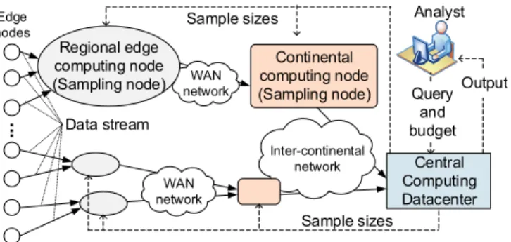
We design and implement APPROXIOT to realize our vision for a low-latency and resource-efficient stream analytics sys-tem based on the above key observations. APPROXIOT recruits the aforementioned edge computing nodes and creates a stream processing pipeline as a logical tree (Figure 1). A data stream traverses over the logical tree towards a centralized cloud or datacenter where the data analysis queries are executed. Along the route to the central location, each node independently selects data items from the input stream while preserving statistical characteristics. The core of APPROXIOT’s design is a novel online sampling algorithm that updates the significance (weight) of those selected data items on each node without any cross-node synchronization. The system can tune the degree of sampling systematically, depending on resource availability and analytics requirements.

Overall, this paper makes the following key contributions. • Approximate computing for IoT-driven stream

ana-lytics. We make a case for approximate computing in IoT, whereby the real-time analysis over the entire data stream is becoming unsustainable due to the gap between the required computing resources and the data volume. • Design and implementation of APPROXIOT (§III and

... Sample sizes Edge nodes Inter-continental network WAN network WAN network Continental computing node (Sampling node) Central Computing Datacenter Analyst Data stream Regional edge computing node (Sampling node) Sample sizes Output Query and budget

Fig. 1. System overview.

weighted hierarchical sampling — based on theoreti-cal foundations. The algorithm needs no coordination across nodes in the system, thereby making APPROXIOT easily parallelizable and hence scalable. Moreover, our algorithm is suitable to process different types of input streams such as long-tailed streams and uniform-speed streams. We prototype APPROXIOT using Apache Kafka. • Comprehensive evaluation of APPROXIOT (§V and

§VI). We evaluate APPROXIOT with synthetic and real-world datasets. Our evaluation results demonstrate that APPROXIOT outperforms the existing approaches. It achieves 1.3×—9.9× higher throughput than the native stream analytics execution, and 3.3×—8.8× higher ac-curacy compared to a simple random sampling scheme.

II. OVERVIEW ANDBACKGROUND A. System Overview

APPROXIOT builds on two design concepts: hierarchical processing and approximate computing. In APPROXIOT, a wide variety of devices or sensors (so-called IoT devices) generate and send data streams to regional edge computing nodes geographically close to themselves. The edge computing clusters managed by local ISPs or content providers sample only a subset of the input data streams and forward them to larger computing facilities such as datacenters. The data streams, again sampled at the datacenters, can be further forwarded to a central location, where a user-specified query is executed and the query results are produced for global-level analysis. These computing clusters spread across the globe form a logical stream processing pipeline as a tree, which is collectively called APPROXIOT. Figure 1 presents the high-level structure of the system.

The design choice of APPROXIOT, i.e., combining ap-proximate computing and hierarchical processing, naturally enables the processing of the input data stream within a specified resource budget. On top of this feature, APPROXIOT produces an approximate query result with rigorous error bounds. In particular, APPROXIOT designs a parallelizable online sampling technique to select and process a subset of data items, where the sample size can be determined based on the resource constraints at each node (i.e., computing cluster), without any cross-node coordination.

Altogether, APPROXIOT achieves three goals.

• Resource efficiency.APPROXIOT utilizes computing and bandwidth resources efficiently by sampling data items at each individual node in the logical tree. If we were to sample data items only at a node where the query is executed, all the computing and bandwidth resources used to process and forward the unused data items would have been wasted.

• Adaptability. The system can adjust the degree of sam-pling based on resource constraints of the nodes. While the core design is agnostic to the ways of choosing the sample size, i.e., whether it is centralized or distributed, this adaptability ensures better resource utilization. • Transparency. For an analyst, the system enables

com-putation over the distributed data in a completely trans-parent fashion. The analyst does not have to manage computational resources; neither does she require any code changes to existing data analytics application/query. B. Technical Building Blocks

APPROXIOT relies on two sampling techniques as the build-ing blocks: stratified samplbuild-ing [6] and reservoir samplbuild-ing [7] because the properties of the two allow APPROXIOT to meet its needs.

1) Stratified Sampling: A sub-stream is the data items from a source. In reality, sub-streams from different data sources may follow different distributions. Stratified sampling was proposed to sample such sub-streams fairly. Here, each sub-stream forms a stratum; if multiple sub-streams follow the same data distribution, they can be combined to form a stratum. For clarity and coherence, hereafter, we still use sub-stream to refer to a stratum.

Stratified sampling receives sub-streams from diverse data sources, and performs the sampling (e.g., simple random sampling [8] or other types of sampling) over each sub-stream independently. In doing so, the data items from each sub-stream can be fairly selected into the sample. Stratified sampling reduces sampling error and improves the precision of the sample. It, however, works only in a situation where it can assume the knowledge of the statistics of all sub-streams (e.g., each sub-stream’s length). This assumption on prior knowledge is unrealistic in practice.

2) Reservoir Sampling: Reservoir sampling is often used to address the unrealistic assumption aforementioned in stratified sampling. It works without the prior knowledge of all the sub-streams. Suppose a system receives a stream consisting of an unknown number of data items. Reservoir sampling maintains a reservoir of size R, and wants to select a sample of (at most)Ritems uniformly at random from the unbounded data stream. Specifically, reservoir sampling keeps the first-received R items in the reservoir. Afterwards, whenever the i-th item arrives (i > R), reservoir sampling keeps this item with probability of N/i and then randomly replaces one existing item in the reservoir. In doing so, each data item in the unbounded stream is selected into the reservoir with equal probability. Reservoir sampling is resource-efficient; however, it could mutilate the statistical quality of the sampled data

Sub-stream, S1

1 2

4 2 3

Reservoir sampling with size, N = 3 Wout 1 = Win1 * 4 / 3 = 4 Wout1 = Win1 = 2 S2 1 2 3 4 Win 1 = 3 1 2 3 4 Win 1 = 3 WWinin22 = 2 = 2 11 22 Node

Upper-node or query execution module Fig. 2. Basic operation at a node.

items in the reservoir especially when the input data stream combines multiple sub-streams with different distributions. For example, the data items received from an infrequent sub-stream could easily get overlooked in reservoir sampling.

III. DESIGN

In this section, we describe the design of APPROXIOT. We first present the basic operation conducted at individual nodes (§III-A). We then discuss how the APPROXIOT system is put together with those nodes (§III-B). We also detail the statistics computation method (§III-C) and the error estimation mechanism (§III-D). Finally, we discuss a design extension to enhance the proposed system (§III-E).

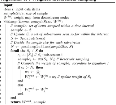
A. Basic Operation: Weighted Hierarchical Sampling The crux of APPROXIOT is the weighted hierarchical sampling algorithm that runs independently on each node and selects a portion from all sub-streams for the sample, without neglecting any single sub-stream. These properties make the algorithm simple and allow it to capture the statistical significance of all sub-streams regardless of their sizes, for which we extend the existing stratified reservoir sampling [9]. Algorithm 1 outlines the weighted hierarchical sampling on a node. The node first stratifies the input stream into sub-streams according to their sources (line 5). It then determines the reservoir size for each sub-stream (line 7), where N denotes a map for the reservoir sizes of all sub-streams. Given Ni for sub-stream Si, the node selects items at random from

Si through the traditional reservoir sampling (line 10). The

reservoir sampling ensures that the number of selected items, ci, fromSi does not exceed its sample sizeNi. Then, a local

weight (wi) for the items selected from Si is:

wi =

(

ci/Ni ifci> Ni

1 ifci≤Ni

(1) Given the input weight (Win

i ) for Si, the node finally

computes an output weight (lines 12-18) as follows: W_iout=

(

Wiin∗wi ifci> Ni

Wiin ifci≤Ni

(2) This process repeats across all sub-streams. Finally, we return the final weight and sample maps (line 20). Figure 2 illustrates how a node applies the reservoir sampling and updates the weight for each sub-stream.

Algorithm 1: : Weighted hierarchical sampling Input:

items: input data items sampleSize: size of sample

Win_{: weight map from downstream nodes} 1 WHSamp(items,sampleSize,Win₎

2 //sample: set of items sampled within a time interval

3 sample← ∅

4 //UpdateS, a set of sub-streams seen so far within the interval

5 S←Update(items)

6 //Decide the sample size for each sub-stream

7 N←getSampleSize(sampleSize,S) 8 forall theSi∈Sdo

9 ci← |Si|//Si: sub-stream i

10 samplei←RS(Si,Ni) //Reservoir sampling

11 //Compute the weight ofsampleiaccording to Equation 1 12 ifci> Nithen

13 wi← Ncii

14 W_iout←W_iin∗wi//update weight ofSi

15 end

16 else

17 Wiout←Wiin

18 end

19 end

20 returnWout,sample

B. Putting It Together

Algorithm 2 presents the overall workflow of APPROXIOT. The algorithm running at each node takes the resourcebudget and parent as input, while that of a root node additionally accepts a user-specified streamingquery. A number of sources generate data items and continuously push them in a streaming fashion through a pre-configured logical tree. Each node in the tree samples data items on a sub-stream basis, based on a specified resource budget. We currently assume there exists a cost function which translates a given query budget (such as the user-specified latency/throughput/accuracy guarantees) into the appropriate sample size for a node in the logical tree. Thereafter, each node (denoted as sampling node in Figure 1) forwards those sampled sub-streams associated with a small amount of metadata to an upper node towards a root node. For sub-streams arriving at the root, the root conducts the sampling of sub-streams, executes the query on the data items, and outputs the query results alongside rigorous error bounds. As shown in Algorithm 2, for each time interval, a node conducts the following steps.

It first derives the sample size (size) based on the given resource budget (line 3). It then extractsΨ, a store that keeps pairs of the metadata (i.e., weight map) and data items for sub-streams that arrive within the interval (line 4). The weight map maintains an up-to-date weight value for each sub-stream. After obtaining a pair of weight map (Win_{) and data items in}

Ψ(line 7), the node runs our weighted hierarchical sampling

(WHSamp), and returns the output weight map,Wout_{, and the}

sampled sub-streams (line 10). If the node is a sampling node (i.e., it has a parent node), then the node sends the sample andWout to its parent node (line 13). Otherwise, it stores the pair of weight map and sampled items in a temporary data structure,Θ(line 16).

Algorithm 2: : APPROXIOT’s algorithm overview Input:

query: streaming query (only for root) budget: resource budget to execute the query parent: successor node

1 begin

2 foreachintervaldo

3 size←costFunction(budget) 4 Ψ←getDataStream(interval) 5 whileΨis not emptydo

6 //Win: Input weight map for sub-streams

7 {Win, items} ←getDataSet(Ψ) 8 //Weighted Hierachical Sampling (§III-A) 9 //Wout: a map of weights of thesample 10 {Wout,sample} ←WHSamp(items,size,Win₎

11 ifparentis not emptythen

12 //(weight, sample) to upstream node

13 Send(parent,Wout_,sample)

14 end 15 else 16 Θ←Θ∪{(Wout_,sample)} 17 end 18 Ψ←Ψ\{(Win, items)} 19 end

20 ifparentis emptythen

21 //Run query as a data-parallel job

22 result←runJob(query,Θ)

23 //Estimate error bounds (§III-D)

24 error←estimateError(result)

25 writeresult±error

26 end

27 end 28 end

processes the query on the data items in Θ. A typical query asks for some statistics such as sum and average of the data streams, whose computation is discussed in §III-C. Finally, it runs an error estimation mechanism (see §III-D) to compute the error bounds for the approximate query result in the form of output±error (lines 21-25).

The entire process repeats for each time interval as the computation window slides [10], [11]. Note that the resource budget may change across time intervals to adapt to user’s requirements.

C. Statistics Computation

The root node conducts the sampling over the incoming items on a time interval basis and computes statistics (such as sum and average) as a query over those sampled items. For any given sub-stream, the node may see multiple pairs of the weight map and sampled items because all nodes in the APPROXIOT sample items and update weights independently with no coordination across them. As denoted in Algorithm 2, Θ contains a series of such pairs across all sub-streams. The root node can then compute an estimate of a sum for the sub-stream as follows: SU Mi= X (Wout i ,Ii)∈Θ ( |Ii| X k=1 Ii,k)·Wiout (3) where Wout

i is a weight value and Ii is a set of items

associated with that weight value for sub-stream Si.

1 2 3 4 w = 1 5 6 2 3 4 w = 1.5 5 2 w = 1.5 5 w = 3 5 Interval u 3 w = 3 3 w = 3 Interval u+1 Time A B C A B C Network Network Reservoir size, n = 4 Reservoir size, n = 1 Reservoir sampling Interval v Interval v w = 3 Interval x 5 3 4 n = 1

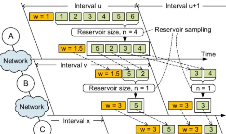
Fig. 3. NodesAandBare sampling nodes that conduct sampling, and node Cis the root node that executes a query. Each node independently maintains intervals. A node (e.g.,A) receives sub-streams (only one sub-stream is shown for brevity) and an interval of a sub-stream contains a series of items and possibly a weight (w). After the reservoir sampling is applied,wis updated based on Algorithm 1. For example, nodeBsamples one out of the two items when the inputwis1.5; thus, the updatedwis1.5×2 = 3. When items arrive within an interval which is different from the interval the input weight arrives, the prior input weight for that sub-stream is used; nodeBsees no weight value associated with items 3 and 4 in the intervalv+ 1. Thus, the node usesw= 1.5and updates the output weight value (w= 1.5×2 = 3).

Suppose there are in total X sub-streams {Si}Xi=1, the approximate total sum of all items received from all sub-streams (denoted asSU M∗) is:

SU M∗=

X

X

i=1

SU Mi (4)

Example.Figure 3 shows how each node individually samples items from a sub-stream and updates its weight value. In the figure, 6 items arrive within an interval at nodeAwhich has a reservoir size of 4. After reservoir sampling, the node updates the weight for the items based on the equation at line 14 in Algorithm 1; thus,w= 1.5. NodeAthen forwards the weight and sampled items to node B.

A weight and its associated items may arrive at different intervals. For instance, in Figure 3, items 3 and 4 arrive at nodeBwithin the intervalv+1while the weight value arrives within the intervalv. For the items 5 and 2, we simply apply Algorithm 1. For the items 3 and 4, we take the weight value (w= 1.5in the figure) used within intervalvfor the same sub-stream and apply the algorithm because the weight value is the up-to-date weight for the sub-stream (as stated previously in

§III-B). Since the reservoir size is half of the number of items in interval v+ 1, the updated weight becomes 1.5×2 = 3; the weight value and the sampled item (in this case, item 3) are then forwarded to nodeC.

Lastly, Θat root node C has two pairs: (3, {item 5}) and (3,{item 3}). Suppose that the index of the item is its value. Then, the estimated sum of the sub-stream is3∗5+3∗3 = 24. Statistical recreation of the original items. We consider two cases: (i) single node and (ii) multiple nodes, in order to discuss how to statistically recreate the original items from the sample and weight map.

(i) Single node case. There is only one node which works as root. All sources send their data streams to the root node. Because the root node solely defines the interval in this setting, there is only one element for each sub-stream in Θ. Thus, Equation (3) is reduced to:

SU Mi= (

|Ii|

X

k=1

Ii,k)·Wiout (5)

whereIi,k denotes the value of thek-th item in setIi.

Initially, when a source generates data items, there is no weight map given to the root node; therefore, the weight of each sub-stream is assumed to be 1 (i.e., Win

i = 1). From

Equation (2) and W_iin = 1, we essentially have W_iout =wi

orW_iout = 1. As a result, Equation (5) represents an unbiased estimate of sub-streamSias it implements the basic reservoir

sampling which is known to obtain a set of unbiased samples from an input stream [12]. Note that, Algorithm 1 works exactly the same way as the one in [9] in this case.

(ii) Multiple nodes case.We extend our notations for further discussion.SU Mi,jis an estimated sum of items in sub-stream

Si at node j. We redefine ci,j, wi,j, Ni,j,Wi,jout and Ii,j in

a similar fashion. We define an upstream pathfor sub-stream Si as a path that items ofSi are forwarded from the original

source to the root node. Letπ(i, j)be a predecessor node (i.e., an immediate lower-level node) of nodejon an upstream path for sub-stream Si.

We consider a set of items of a sub-stream arriving at a bottom/leaf node (i.e., the node contacted by data sources) within an interval as the original data set (i.e., ground truth). For instance, in Figure 3, node A is the bottom node and items 1-6 form an original set. An original set can be split into a number of (Wout

i , Ii) pairs as items in the original

set arrive in different time intervals when they traverse nodes in a logical tree. To facilitate our analysis only, we assume that those (Wout

i , Ii) pairs arrive at the root node within the

same interval. This assumption allows us to trace back the original set represented by the (W_iout, Ii) pairs seen at the

root node. In practice, the APPROXIOT system works without this assumption since the ground truth is unknown.

LetGTi,bbe the sum of the original set seen at bottom node

b, andSU Mi,r be the estimate at root noder. We now show

GTi,b'SU Mi,r. GTi,b= |Ii,b| X k=1 Ii,b,k (6)

where Ii,b,k is the k-th item from the original set at bottom

node bfor sub-stream Si.

From Equation (3), SU Mi,r can be simply rewritten as:

SU Mi,r= X (Wout i,r ,Ii,r)∈Θ ( |Ii,r| X k=1

Ii,r,k)·Wi,rout

(7)

The reservoir sampling executed at each node creates suffi-cient randomness for the selected items. However, there is one

invariant — the estimate on the total number of items in the original set should be correct. Suppose that the value of all items is 1, i.e.,Ii,b,k = 1for allk. Then,GTi,b=|Ii,b|=ci,b

and SU Mi,r = P(Wout

i,r ,Ii,r)∈Θ|Ii,r| ·W out

i,r . Therefore, we

need to show that the following holds: X

(Wout i,r ,Ii,r)∈Θ

|Ii,r| ·Wi,rout=ci,b. (8)

For this, it is necessary to show thatWout

i,j ·cfi,j=W

in i,j·ci,j

on nodej wherec_fi,j is the number of sampled items after the

reservoir sampling.

Proof:According to Algorithm 1,

W_i,jout = (

Wi,jin·ci,j/Ni,j if ci,j > Ni,j

W_i,jin if ci,j ≤Ni,j

(9)

If ci,j > Ni,j, c_fi,j = Ni,j. Then, Wi,jout ·cfi,j = W

in i,j ·

ci,j/Ni,j·Ni,j =Wi,jin·ci,j. If ci,j ≤Ni,j,c_fi,j=ci,j. Thus,

Wout

i,j ·cfi,j=W

in

i,j·ci,j.

If there is no split of the sampled items as they traverse nodes,P

(Wout

i,r ,Ii,r)∈Θ|Ii,r|·W out

i,r is equivalent to|Ii,r|·Wi,rout.

Since|Ii,r|=cfi,j,W

out

i,r ·cfi,j=W

in

i,j·ci,j. We also know that

Win

i,j·ci,j =W_i,πout_(i,j)·c^i,π(i,j). After we recursively rewrite the previous quantity, we obtainW_i,bin·ci,b, becauseWi,bin= 1,

W_i,rout·c_fi,j=ci,b.

If the items of Si from node π(i, j) are split across

m intervals at node j starting from interval u, c_^i,π(i,j) = Pu+m−1

t=u ci,j,t where ci,j,t is the number of items of Si

arriving at node j at interval t. Since W_i,jin = W_i,πout_(i,j), Wout

i,π(i,j)·c^i,π(i,j)=Wi,jin·

Pm+u−1

t=u ci,j,t. Hence, the previous

recursion method can be applied here, too. As a result, Equation (8) holds true even when the items of a sub-stream are split across intervals at nodes.

D. Error Estimation

We now describe a method to estimate the accuracy of our approximate results with rigorous error bounds. Suppose there are X sub-streams {Si}Xi=1 composing the input stream. We compute, at root node r, the approximate sum of all items received from all sub-streams. As each sub-stream is sampled independently, the variance of the approximate sum is:

V ar(SU M∗,r) = X

X

i=1

V ar(SU Mi,r) (10)

Further, as items are randomly selected across nodes for a sample within each sub-stream, we can apply the random sampling theory (central limit theorem) [13]. Hence, the variance of the approximate sum is estimated as:

d V ar(SU M∗,r) = X X i=1 ci,b·(ci,b−ζ)· s2 i,r ζ (11)

where ζ =P (Wout

i,r ,Ii,r)∈Θ|Ii,r|. From Equation (8), we can

obtain ci,b. In addition, si,r denotes the standard deviation of

the sub-stream Si’s sampled items at root noder:

s2i,r = 1 ζ−1 · ζ X k=1 (Ii,r,k−I¯i,r)2 (12) whereI¯i,r= 1_ζ ·P ζ k=1Ii,r,k.

Next, we show how we can similarly estimate the variance of the approximate mean of all items received from all theX sub-streams. The approximate mean can be computed as:

M EAN∗,r= SU M∗,r PX i=1ci,b = PX

i=1ci,b·M EANi,r

PX i=1ci,b = X X i=1 (ϕi·M EANi,r) (13) Here,ϕi= ci,b PX

i=1ci,b. Then, as each sub-stream is sampled

independently, according to the random sampling theory [13], the variance of the approximate mean can be estimated as:

d

V ar(M EAN∗,r) = X

X

i=1

V ar(ϕi·M EANi,r)

=

X

X

i=1

ϕ2_i ·V ar(M EANi,r)

= X X i=1 ϕ2_i · s 2 i,r ζ · ci,b−ζ ci,b (14)

Error bound. We compute the error bound for the approx-imate result based on the “68-95-99.7” rule [14]. According to this rule, the approximate result is within one, two, and three standard deviations away from the exact result with probabilities of 68%, 95%, and 99.7%, respectively. The standard deviation is computed by taking the square root of the variance in Equation (11) and Equation (14), respectively, for computing approximate sum and mean.

E. Distributed Execution

Our proposed algorithm naturally extends for distributed execution as it does not require synchronization. Our straight-forward design extension for parallelization is as follows: we handle each sub-stream by a set of w worker nodes. Each worker node samples an equal portion of items from this sub-stream and generates a local reservoir of size no larger than Ni/w, whereNi is the total reservoir size allocated for

sub-stream Si. In addition, each worker node maintains a local

counter to measure the number of its received items within a concerned time interval for weight calculation. The rest of the design remains the same.

IV. IMPLEMENTATION

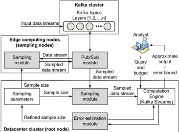
We implemented APPROXIOT using Apache Kafka [15] and its library Kafka Streams [16]. Figure 4 illustrates the high-level architecture of our prototype, where the shaded boxes represent the implemented modules. In this section, we first

Computation Engine (Kafka Streams) Sampling module Error estimation module Sampling parameters Pub/Sub module Sampling module Analyst Sample size Sampled data stream Data stream

...

...

...

Kafka cluster Kafka topics Layers n]

Edge computing nodes (sampling nodes)

Datacenter cluster (root node) Sample size

Refined sample size

Sampled data stream Sampled data stream Query and budget Approximate output + error bound

Fig. 4. APPROXIOT architecture.

give a necessary background about Apache Kafka, and we next present the implementation details.

A. Background

Apache Kafka [15] is a widely used scalable fault-tolerant distributed pub/sub messaging platform. Kafka offers the re-liable distributed queues called topics to receive input data streams. Stream analytics systems can subscribe these topics to retrieve and process data streams. We used Kafka to model the layers in the edge computing topology, where the input streams are pipelined across layers via pre-defined topics.

Recently, Kafka Streams [16] has been developed as a library on top of Kafka to offer a high-level dataflow API for stream processing. The key idea behind Kafka Streams is that it considers an input stream as an append-only data table (a log). Each arriving data item is considered as a row appended to the table. This design enables Kafka Streams to be a real-time stream processing engine, as opposed to the batched based stream processing systems (e.g., Spark Streaming [2]) that treat the input data stream as a sequence of micro-batches. Furthermore, since Kafka Streams is built on top of Kafka, it requires no additional cluster setup for a stream processing system (e.g., Apache Flink [17], Storm [18]). For these advantages, Kafka Streams is an excellent choice for our prototype implementation.

The Kafka Streams library supports two sets of APIs [16]: (i)High-Level Streams DSL (Domain Specific Language) API to build a processing topology (i.e., DAG dataflow) and (ii) Low-Level Processor API to create user-defined processors (a processor is an operator in the processing topology).

B. APPROXIOT Implementation Details

At a high level (see Figure 4), the input data streams are ingested to a Kafka cluster.

Edge computing nodes (sampling nodes).A sampling node consumes an input stream from the Kafka cluster via the Pub/Sub module by subscribing to a pre-defined topic. There-after, the sampling module samples the input stream in an

online manner using the proposed sampling algorithm (§III). Next, a producer is used to push the sampled data items to the next layer in the edge computing network topology using the Kafka topic of the next layer.

Datacenter cluster (root node). The root node receives the sampled data streams from the final layer of sampling nodes. First, it also makes use of the sampling module to take a sample of the input. Thereafter, the computation engine of Kafka Streams (High-Level Streams DSL processors) executes the input query over the sampled data stream to produce an approximate output. Finally, the error estimation module per-forms the error estimation mechanism (see §III-D) to provide a rigorous error bound for the approximate query result. In addition, in the case the error bound of the approximate result exceeds the desired budget of the user, an adaptive feedback mechanism is activated to refine the sampling parameters at all layers to improve the accuracy in subsequent runs. We next describe in detail the implemented modules.

I: Pub/Sub module. The Pub/Sub module ensures the com-munication between the edge computing layers. For that, we made use of the High-Level Streams DSL API to create the producer and consumer processors to send and retrieve data streams through a pre-defined topic corresponding to the layer. II: Sampling module.The sampling module implements the algorithm described in §III. In particular, we implemented the algorithm in a user-defined processor (i.e., sampling processor) using the Low-Level API supported by Kafka. The sampling processor works as a normal processor in the Kafka computing topology to select input data items from the topics.

In addition, for the baseline comparison, we also imple-mented a simple random sampling (SRS) algorithm into a user-defined processor using the coin flip sampling algorithm [19]. III: Error estimation module. The error estimation module computes the error bounds for the approximate output, which is necessary for the user to interpret the accuracy of result. We used the Apache Common Math library [20] to implement the error estimation mechanism as described in §III-D.

V. EVALUATION: MICROBENCHMARKS

In this section, we present the evaluation results of APPROX -IOT using microbenchmarks. In the next section, we describe the evaluation results based on real-world datasets.

A. Experimental Setup

Cluster setup.We deployed the APPROXIOT system using a cluster of25nodes. We used15nodes for the IoT deployment, each equipped with two dual-core Intel Xeon E3-1220 v3 processors and 4GB of RAM, running Ubuntu 14.04. In the deployment, we emulated a four-layer tree topology of an IoT infrastructure which contains 8 source nodes producing the input data stream,4nodes for the first edge computing layer,2 nodes for the second edge computing layer, and one datacenter node (the root node). For the communication between the edge computing layers, we used a Kafka cluster using the

0 0.1 0.2 0.3 0.4 0.5 0.6 10 20 40 60 80 90 A c c u ra c y l o s s ( % ) Sampling fraction (%) ApproxIoT SRS

(a) Gaussian distribution

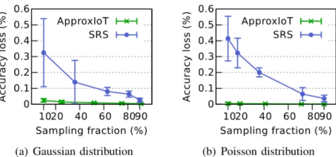
0 0.1 0.2 0.3 0.4 0.5 0.6 10 20 40 60 80 90 A c c u ra c y l o s s ( % ) Sampling fraction (%) ApproxIoT SRS (b) Poisson distribution Fig. 5. Accuracy loss vs sampling fraction. The accuracy loss of ApproxIoT is at most0.035%in (a) and0.013%in (b), both of which are smaller than the counterpart of SRS.

10remaining nodes, each of which has3-core Intel Xeon E5-2603 v3 processors and8GB of RAM, running Ubuntu14.04. To emulate a WAN environment, we used the tc (traffic control) tool [21]. Based on the real measurements [22], the round-trip delay times between two adjacent layers are set to 20ms (between the source node and the first edge computing layer),40ms (between the first layer and the second layer) and 80ms (between the second layer and the datacenter node). In the network, each link’s capacity is1Gbps. This WAN setting remains the same across all the experiments we conducted unless otherwise stated.

Synthetic data stream. We evaluated the performance of APPROXIOT using synthetic input data streams with two data distributions: Gaussian and Poisson. For the Gaussian distribution, we generated four types of input sub-streams:

A (µ = 10, σ = 5), B (µ = 1000, σ = 50), C (µ = 10000, σ = 500) and D (µ = 100000, σ = 5000). For the Poisson distribution, we used four types of input sub-streams:

A(λ= 10),B(λ= 100),C (λ= 1000) andD(λ= 10000). Metrics.We evaluated the performance of APPROXIOT with the following three metrics: (i) Throughput defined as the number of data items processed per second; (ii) Accuracy loss defined as |approx−exact|/exact, where approx and exact denote the results produced by APPROXIOT and a native execution without sampling, respectively; and lastly, (iii) Latencydefined as the end-to-end latency taken by a data item from the source until it is processed in the datacenter. Methodology.We used the source nodes to produce and tune the rate of the input data streams such that the datacenter node in APPROXIOT was saturated. This input rate was used for three approaches: (i) APPROXIOT, (ii) SRS-based system employing Simple Random Sampling (in short, SRS), and(iii) Native execution. In the native execution approach, the input data streams are transferred from the source nodes all the way to the datacenter without any sampling at the edge nodes. B. Effect of Varying Sampling Fractions

Accuracy.We first evaluate the accuracy loss of APPROXIOT and the SRS-based system. We use both Gaussian and Poisson distributions while we vary the sampling fractions.

Figure 5 shows that APPROXIOT achieves much higher accuracy than the SRS-based system for both datasets. In

0 50 100 150 10 20 40 60 80 100 T h ro u g h p u t( K )# it e m s /s Sampling fraction (%) ApproxIoT SRS Native

Fig. 6. Throughput vs sampling frac-tion. 0 20 40 60 80 100 10 20 40 60 80 100 B W s a v in g r a te ( % ) Sampling fraction (%) ApproxIoT SRS

Fig. 7. Bandwidth saving vs sampling fraction.

particular, when the sampling fraction is 10%, the accuracy of APPROXIOT is 10×and 30×higher than SRS’s accuracy for Gaussian and Poisson datasets, respectively. This higher accuracy of APPROXIOT is because APPROXIOT ensures data items from each sub-stream are selected fairly by leveraging stratified sampling. Here, the absolute accuracy loss in SRS may look insignificant, but the estimation of SRS can be completely useless in the presence of a skewed distribution of arrival rates of the input streams, which we show in§V-E. Throughput.We next evaluate the throughput of APPROXIOT in comparison with the SRS-based system.

Figure 6 depicts the throughput comparison between AP -PROXIOT and SRS. APPROXIOT achieves a similar throughput as SRS due to the fact that the proposed sampling mechanism, just like SRS, requires no synchronization between workers (CPU cores) to take samples from the input data stream. For instance, with the sampling fraction of 89%, the throughput of APPROXIOT is 12429 items/s, and that of SRS is 12547 items/s with the sampling fraction of 90%. Note that, as we perform sampling across different layers, we cannot ensure that two algorithms have the same sampling fraction.

Figure 6 also shows that both APPROXIOT and SRS have a similar throughput compared to the native execution even when the sampling fraction is 100%. APPROXIOT, SRS and the native execution achieve 11003 items/s, 11046 items/s and 11134 items/s, respectively. This demonstrates the low overhead of our sampling mechanism.

Network bandwidth. In addition, sampling ensures that AP -PROXIOT (and SRS, too) significantly saves the network bandwidth between the computing layers as shown in Figure 7; the network resource is fully utilized in this case, so the sampling fraction of 10% means that our system only requires 10% of the total capacity (e.g., 100 Mbps out of 1 Gbps). Thus, even when the network resource is limited, APPROXIOT can function effectively.

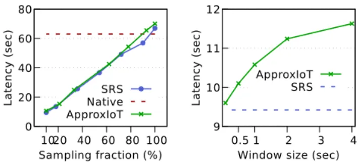
Latency. We set the window size of APPROXIOT to one second. Figure 8 shows that APPROXIOT incurs a similar latency compared to the SRS-based system. In addition, when the sampling fraction of APPROXIOT is 10%, APPROXIOT achieves a6×speedup with respect to the native execution.

0 20 40 60 80 10 20 40 60 80 100 L a te n c y ( s e c ) Sampling fraction (%) SRS Native ApproxIoT

Fig. 8. Latency vs sampling fraction.

APPROXIOT uses1second window.

9 10 11 12 0.5 1 2 3 4 L a te n c y ( s e c )

Window size (sec) ApproxIoT

SRS

Fig. 9. Latency vs window size. Sam-pling fraction is set to 10%. C. Effect of Varying Window Sizes

The previous window size of one second may look arbitrary. Thus, we evaluate the impact of varying window sizes on the latency of APPROXIOT. We set a fixed sampling fraction of 10% and measure the latency of the evaluated systems while we vary window sizes. Figure 9 shows the latency compar-ison between APPROXIOT and the SRS-based system. The latency of APPROXIOT increases as the window size increases whereas the latency of the SRS-based system remains the same. This is because the SRS-based system does not require a window for sampling the input streams in any of the edge computing layers. Therefore, like in any other window-based streaming systems [2], [17], the operators have to set small window sizes to meet the low latency requirement.

D. Effect of Fluctuating Input Rates of Sub-streams

We next evaluate the impact of fluctuating rates of sub-streams on the accuracy of APPROXIOT. We keep the sam-pling fraction of 60% and measure the accuracy loss of AP -PROXIOT and the SRS-based system. Figures 10(a) and 10(b) present the accuracy loss of APPROXIOT and SRS with Gaussian distribution and Poisson distribution datasets. For these experiments, we create three different settings, in each of which four sub-streamsA,B,CandDhave different arrival rates. A setting is expressed as (A:B:C:D). For example, (50k : 25k : 12.5k : 625) means that the input rates of sub-streams A, B, C andD are 50k items/s, 25k items/s, 12.5k items/s, and625 items/s, respectively.

Both figures show that the accuracy of these approaches improves proportionally to the input rate of the sub-stream

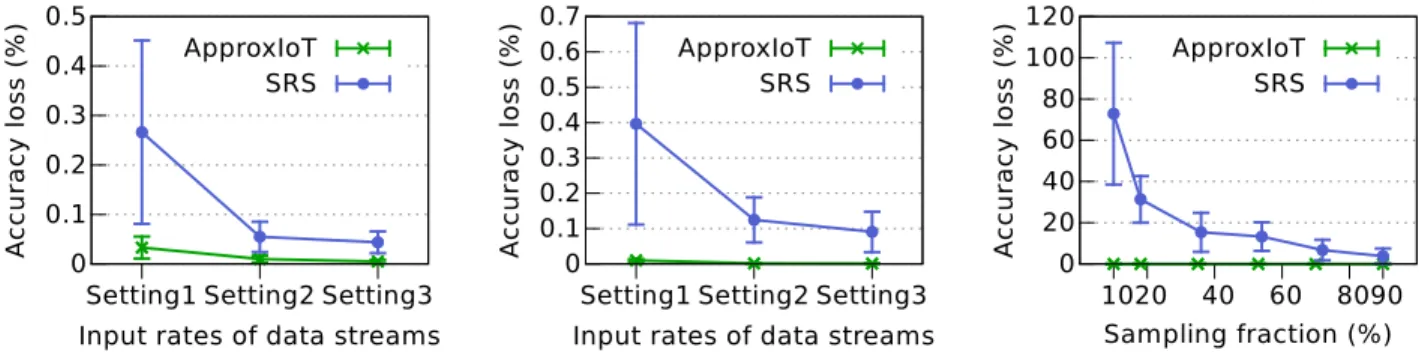
Dsince data items of this sub-stream have significant values compared to other sub-streams. Across all settings, APPROX -IOT achieves higher accuracy than the SRS-based system. For instance, under Setting1 in Figure 10(a), the accuracy loss of SRS-based system is 5.5×higher than that of APPROXIOT; while under the same setting in Figure 10(b), the accuracy of APPROXIOT is 74×higher than that of the SRS-based system. The higher accuracy of APPROXIOT against SRS is due to the similar reason that we already explained: the SRS-based system may overlook the sub-stream D in which there are only a few data items but their values are significant, whereas APPROXIOT is based on stratified sampling, and therefore, it captures all of the sub-streams well.

0 0.1 0.2 0.3 0.4 0.5

Setting1 Setting2 Setting3

A c c u ra c y l o s s ( % )

Input rates of data streams ApproxIoT

SRS

(a) Gaussian distribution

0 0.1 0.2 0.3 0.4 0.5 0.6 0.7

Setting1 Setting2 Setting3

A c c u ra c y l o s s ( % )

Input rates of data streams ApproxIoT SRS (b) Poisson distribution 0 20 40 60 80 100 120 10 20 40 60 80 90 A c c u ra c y l o s s ( % ) Sampling fraction (%) ApproxIoT SRS

(c) Extremely skewed input data stream Fig. 10. The accuracy comparison between APPROXIOT and the SRS-based system with different arrival rates of sub-streams. For (a) and (b), the arrival rates (items/sec) of the four input sub-streamsA,B,C, andDare the following: Setting1: (50k: 25k: 12.5k: 625), Setting2: (25k: 25k: 25k: 25k) and Setting3: (625 : 12.5k: 25k: 50k). For (c), Poisson distribution is used;A,B,CandDhaveλ= 10,100,1000and10000000, respectively; the sub-streamAaccounts for80%of all data items while the sub-streamsB,CandDaccount for only19.89%,0.1%, and0.01%, respectively. The average accuracy loss of APPROXIOT is at most0.056%in (a),0.014%in (b) and0.035%in (c).

E. Effect of Skew in Input Data Stream

In this experiment, we analyze the effect of skew in the input data stream. We create a sub-stream that dominates the other sub-streams in terms of the number of data items. In particular, we generate an input data stream that consists of four sub-streams following a Poisson distribution, namely A

(λ= 10),B(λ= 100),C(λ= 1000), andD(λ= 10000000). In this input data stream, the sub-stream Aaccounts for80% of all data items, whereas the sub-streamsB,CandDrepresent only19.89%,0.1%, and0.01%, respectively.

Figure 10(c) shows that APPROXIOT achieves a signifi-cantly higher accuracy than the SRS-based system. With the sampling fraction of 10%, the accuracy of APPROXIOT is 2600× higher than the accuracy of SRS-based system. The reason for this is that APPROXIOT considers each sub-stream fairly — none of them is ignored when samples are taken. Meanwhile, the SRS-based system may not yield sufficient numbers of data items for each sub-stream. Interestingly, as highlighted in Figure 10(c), the SRS-based system may overestimate the sum of the input data stream since it by chance mainly considers sub-streamDand ignores others (see evaluation results with the sampling fraction of 10%).

VI. EVALUATION: REAL-WORLDDATASETS In this section, we evaluate APPROXIOT using two real-world datasets:(i)New York taxi ride and(ii)Brasov pollution dataset. We used the same cluster setup as described in §V-A. A. New York Taxi Ride Dataset

Dataset.The NYC taxi ride dataset has been published at the DEBS 2015 Grand Challenge [23]. This dataset consists of the ride information of10,000taxies in New York City in 2013. We used the dataset from January 2013.

Query. We performed the following query: What is the total payment for taxi fares in NYC at each time window?

Results.Figure 11(a) shows that the accuracy of APPROXIOT improves with the increase of sampling fraction. With the sampling fraction of10%, the accuracy loss of APPROXIOT is 0.1%, whereas with the sampling fraction of47%, the accuracy

0 0.04 0.08 0.12 0.16 10 20 40 60 80 90 A c c u ra c y l o s s ( % ) Sampling fraction (%) Brasov Pollution NYC Taxi

(a) Accuracy loss vs sampling frac-tion 0 50 100 150 10 20 40 60 80 100 Native throughput for two datasets

T h ro u g h p u t( K )# it e m s /s Sampling fraction (%) Brasov Pollution NYC Taxi

(b) Throughput vs sampling fraction

Fig. 11. The accuracy loss and throughput of APPROXIOT in processing the two real-world datasets. The flat line in (b) shows the throughput of the native approach for processing the two datasets; only one line is presented because there is a marginal difference between processing the two datasets.

loss is only 0.04%. In addition, we measure the throughput of APPROXIOT with varying sampling fractions. Figure 11(b) depicts that the throughput of APPROXIOT reduces when the sampling fraction increases. With the sampling fraction of 10%, the throughput of APPROXIOT is 122,199 items/sec, which is roughly 10%higher than the native execution. B. Brasov Pollution Dataset

Dataset. The Brasov pollution dataset [24] consists of the pollution measurements (e.g., air quality index) in Brasov, Romania from August 2014 to October 2014. Each sensor provides a measurement result every5 minutes.

Query. We performed the following query:What is the total pollution values of particulate matter, carbon monoxide, sulfur dioxide and nitrogen dioxide in every time window?

Results.Figure 11(a) depicts the accuracy loss of APPROXIOT in processing the pollution dataset with varying sampling fractions. With the sampling fractions of 10% and 40%, the accuracy loss of APPROXIOT are 0.07% and 0.02%, respectively. The accuracy loss in processing this dataset has a similar but lower curve as for the NYC taxi ride dataset. The reason is that the values of data items in Brasov pollution dataset are more stable than in NYC tax ride dataset.

Figure 11(b) presents the throughput of APPROXIOT with different sampling fractions. With the sampling fraction of 10%, APPROXIOT achieves a9×higher throughput than the native execution. The throughputs of processing both the NYC taxi ride dataset and the pollution dataset are similar.

VII. RELATEDWORK

With the ability to enable a systematic trade-off between accuracy and efficiency, approximate computing has been explored in the context of distibuted data analytics [25], [26], [27], [28], [29], [9]. In this context, sampling-based techniques are properly the most widely used for approximate data analytics [25], [26], [27]. These systems show that it is possible to leverage the benefits of approximate computing in the distributed big data analytics settings. Unfortunately, these systems are mainly targeted towards batch processing, where the input data remains unchanged during the course of sampling. Therefore, these systems cannot cater to stream analytics, which requires real-time processing of data streams. To overcome this limitation, IncApprox [28], and StreamApprox [9], [30] have been proposed for approximate stream analytics. IncApprox introduces an online “biased sam-pling” algorithm that uses self-adjusting computation [31] to produce incrementally updated approximate results [32], [33], [34], [35]. Meanwhile, StreamApprox handles the fluctuation of input streams by using an online adaptive stratified sampling algorithm. These systems demonstrate that it’s also possible to trade the output quality for efficiency in stream process-ing. Unfortunately, these systems target processing input data streams within a centralized datacenter, where the online sampling is carried out at a centralized stream aggregator. In APPROXIOT, we designed a distributed online sampling algorithm for the IoT setting, where the sampling is carried out in a truly distributed fashion at multiple levels using the edge computing resources.

Recently, in the context of IoT,edge computinghas emerged as a promising solution to reduce latency in data analytics systems [36], [37]. In edge computing, a part of computation and storage are performed at the Internet’s edge closer to IoT devices or sensors. By moving either whole or partial computation to the edge, edge computing allows to achieve not only low latency but also significant reduction in bandwidth consumption [37]. Several works deploy sampling and filtering mechanisms at sources (sensor nodes) to further optimize communication costs [38], [39]. However, the proposed sam-pling mechanisms in these works are “snapshot samsam-pling” techniques which are used to take input data stream every certain time interval. PrivApprox [29], [40] proposed a mar-riage of approximate computing based on sampling with the randomized response for improved performance and users’ privacy. As opposed, in APPROXIOT, we leverage sampling-based techniques at the edge to further reduce the latency and bandwidth consumption in processing large-scale IoT data. In detail, we design an online adaptive random sampling algorithm, and perform it not only at the root node, but also at all layers of the computing topology.

Finally, it is worth to mention that there has been a surge of research in geo-distributed data analytics in multi-datacenters [41], [42], [43]. However, these system focus on improving the performance for batch processing in the context of data centers, and are not designed for edge computing. In APPROXIOT, we design an approximation technique for real-time stream analytics in a geo-distributed edge computing.

VIII. CONCLUSION

The unprecedentedly huge volume of data in the IoT era presents both opportunities and challenges for building data-driven intelligent services. The current centralized computing model cannot cope with low-latency requirement in many online services, and it is also a wasteful computing medium in terms of networking, computing, and storage infrastruc-ture for handling IoT-driven data streams across the globe. In this paper, we explored a radically different approach that exploits approximate computing paradigm for a globally distributed IoT environment. We designed and implemented APPROXIOT, a stream analytics system for IoT that achieves efficient resource utilization, and also adapts to the varying requirements of analytics applications and constraints in the underlying computing/networking infrastructure. The nodes in the system run a weighted hierarchical sampling algorithm independently without any cross-node coordination, which facilitates parallelization, thereby making APPROXIOT scal-able. Our evaluation with synthetic and real-world datasets demonstrates that APPROXIOT achieves 1.3×—9.9× higher throughput than the native stream analytics execution and 3.3×—8.8×higher accuracy than a simple random sampling scheme under the varying sampling fractions of80%to10%. Limitations and future work.While APPROXIOT approach is quite useful to achieve desired properties, our current system implementation has the following limitations.

First, APPROXIOT currently supports only approximate linear queries. We plan to extend the system to support more complex queries [44], [27] such as joins, top-k, etc., as part of the future work.

Second, our current implementation relies on manual ad-justment of user’s query budget to the required sampling parameters. As part of the future work, we plan to implement an automated cost function to tune the sampling parameters for the required system performance and resource utilization. Lastly, we have evaluated APPROXIOT using a small testbed. As part of the future work, we plan to extend our system evaluation via deploying APPROXIOT over Azure Stream Analytics [45] to further evaluate the performance of our system in a real IoT infrastructure.

The source code of APPROXIOT is publicly available: https: //ApproxIoT.github.io/ApproxIoT/

ACKNOWLEDGMENT

We thank our shepherd Grace Lewis for her comments and suggestions. This work was in part supported by EPSRC grants EP/L02277X/1, EP/N033981/1, Alan Turing Institute, and Amazon AWS Research Grant.

REFERENCES

[1] Cisco, “Cisco Global Cloud Index: Forecast and Methodology,” inCisco White Paper, 2016.

[2] “Apache Spark Streaming,” http://spark.apache.org/streaming, accessed: April, 2018.

[3] Garcia Lopezet al., “Edge-centric computing: Vision and challenges,” inProceedings of SIGCOMM CCR, 2015.

[4] A. Doucet, S. Godsill, and C. Andrieu, “On sequential monte carlo sampling methods for bayesian filtering,” Statistics and Computing, 2000.

[5] S. Natarajan,Imprecise and Approximate Computation. Kluwer Aca-demic Publishers, 1995.

[6] M. Al-Kateb and B. S. Lee, “Stratified reservoir sampling over hetero-geneous data streams,” inProceedings of the 22nd International Con-ference on Scientific and Statistical Database Management (SSDBM), 2010.

[7] J. S. Vitter, “Random sampling with a reservoir,”ACM Transactions on Mathematical Software (TOMS), 1985.

[8] S. Lohr,Sampling: design and analysis, 2nd Edition. Cengage Learning, 2009.

[9] D. L. Quoc, R. Chen, P. Bhatotia, C. Fetzer, V. Hilt, and T. Strufe, “StreamApprox: Approximate Computing for Stream Analytics,” in

Proceedings of the International Middleware Conference (Middleware), 2017.

[10] P. Bhatotia, U. A. Acar, F. P. Junqueira, and R. Rodrigues, “Slider: Incremental Sliding Window Analytics,” in Proceedings of the 15th International Middleware Conference (Middleware), 2014.

[11] P. Bhatotia, M. Dischinger, R. Rodrigues, and U. A. Acar, “Slider: Incre-mental Sliding-Window Computations for Large-Scale Data Analysis,” MPI-SWS, Tech. Rep. MPI-SWS-2012-004, 2012, http://www.mpi-sws. org/tr/2012-004.pdf.

[12] C. C. Aggarwal, “On biased reservoir sampling in the presence of stream evolution,” inProceedings of the 32nd International Conference on Very Large Data Bases, 2006.

[13] S. K. Thompson,Sampling. Wiley Series in Probability and Statistics, 2012.

[14] F. Pukelsheim, “The three sigma rule,” in The American Statistician, 1994.

[15] “Kafka - A high-throughput distributed messaging system,” http://kafka. apache.org, accessed: April, 2018.

[16] “Kafka Streams API,” https://kafka.apache.org/documentation/streams/, accessed: April, 2018.

[17] “Apache Flink,” https://flink.apache.org/, accessed: April, 2018. [18] “Apache Storm,” http://storm-project.net/, accessed: May, 2017. [19] C. Jermaine, S. Arumugam, A. Pol, and A. Dobra, “Scalable

Approx-imate Query Processing with the DBO Engine,”ACM Transactions of Database Systems (TODS), 2008.

[20] C. Math, “The Apache Commons Mathematics Library,” http:// commons.apache.org/proper/commons-math, accessed: May, 2017. [21] B. Hubert et al., “Linux advanced routing & traffic control howto,”

setembro de, 2002.

[22] “IP Latency Statistics,” http://www.verizonenterprise.com/about/ network/latency/, accessed: April, 2018.

[23] Z. Jerzak and H. Ziekow, “The debs 2015 grand challenge,” in Proceed-ings of the 9th ACM International Conference on Distributed Event-Based Systems (DEBS), 2015.

[24] M. I. Ali, F. Gao, and A. Mileo, “Citybench: A configurable benchmark to evaluate rsp engines using smart city datasets,” inIn proceedings of 14th International Semantic Web Conference (ISWC), 2015.

[25] S. Agarwal, B. Mozafari, A. Panda, H. Milner, S. Madden, and I. Stoica, “BlinkDB: Queries with Bounded Errors and Bounded Response Times on Very Large Data,” inProceedings of the ACM European Conference on Computer Systems (EuroSys), 2013.

[26] I. Goiri, R. Bianchini, S. Nagarakatte, and T. D. Nguyen, “Approx-Hadoop: Bringing Approximations to MapReduce Frameworks,” in

Proceedings of the Twentieth International Conference on Architectural

Support for Programming Languages and Operating Systems (ASPLOS), 2015.

[27] S. Kandula, A. Shanbhag, A. Vitorovic, M. Olma, R. Grandl, S. Chaud-huri, and B. Ding, “Quickr: Lazily Approximating Complex Ad-Hoc Queries in Big Data Clusters,” inProceedings of the ACM SIGMOD International Conference on Management of Data (SIGMOD), 2016. [28] D. R. Krishnan, D. L. Quoc, P. Bhatotia, C. Fetzer, and R. Rodrigues,

“IncApprox: A Data Analytics System for Incremental Approximate Computing,” in Proceedings of the 25th International Conference on World Wide Web (WWW), 2016.

[29] D. L. Quoc, M. Beck, P. Bhatotia, R. Chen, C. Fetzer, and T. Strufe, “PrivApprox: Privacy-Preserving Stream Analytics,” inProceedings of the 2017 USENIX Annual Technical Conference (USENIX ATC), 2017. [30] D. L. Quoc, R. Chen, P. Bhatotia, C. Fetze, V. Hilt, and T. Strufe, “Approximate Stream Analytics in Apache Flink and Apache Spark Streaming,”CoRR, vol. abs/1709.02946, 2017.

[31] P. Bhatotia, “Incremental parallel and distributed systems,” Ph.D. disser-tation, Max Planck Institute for Software Systems (MPI-SWS), 2015. [32] P. Bhatotia, R. Rodrigues, and A. Verma, “Shredder: GPU-Accelerated

Incremental Storage and Computation,” in Proceedings of USENIX Conference on File and Storage Technologies (FAST), 2012.

[33] P. Bhatotia, A. Wieder, R. Rodrigues, U. A. Acar, and R. Pasquini, “Incoop: MapReduce for Incremental Computations,” inProceedings of the ACM Symposium on Cloud Computing (SoCC), 2011.

[34] P. Bhatotia, A. Wieder, I. E. Akkus, R. Rodrigues, and U. A. Acar, “Large-scale incremental data processing with change propagation,” in

Proceedings of the Conference on Hot Topics in Cloud Computing (HotCloud), 2011.

[35] P. Bhatotia, P. Fonseca, U. A. Acar, B. Brandenburg, and R. Rodrigues, “iThreads: A Threading Library for Parallel Incremental Computation,” in proceedings of the 20th International Conference on Architectural Support for Programming Languages and Operating Systems (ASPLOS), 2015.

[36] M. Satyanarayanan, “The emergence of edge computing,” Computer, 2017.

[37] H. Chang, A. Hari, S. Mukherjee, and T. V. Lakshman, “Bringing the cloud to the edge,” inProceedings of the IEEE Conference on Computer Communications Workshops (INFOCOM WKSHPS), 2014.

[38] J. Traub, S. Breß, T. Rabl, A. Katsifodimos, and V. Markl, “Optimized on-demand data streaming from sensor nodes,” in Proceedings of the 2017 Symposium on Cloud Computing (SoCC), 2017.

[39] D. Trihinas, G. Pallis, and M. D. Dikaiakos, “AdaM: An adaptive monitoring framework for sampling and filtering on IoT devices,” in

2015 IEEE International Conference on Big Data (Big Data), 2015. [40] D. L. Quoc, M. Beck, P. Bhatotia, R. Chen, C. Fetzer, and T. Strufe,

“Privacy preserving stream analytics: The marriage of randomized response and approximate computing,” https://arxiv.org/abs/1701.05403, 2017. [Online]. Available: https://arxiv.org/abs/1701.05403

[41] R. Viswanathan, G. Ananthanarayanan, and A. Akella, “CLARINET: Wan-aware optimization for analytics queries,” inProceedings of the 12th USENIX Symposium on Operating Systems Design and Implemen-tation (OSDI), 2016.

[42] K. Kloudas, M. Mamede, N. Preguic¸a, and R. Rodrigues, “Pixida: Opti-mizing Data Parallel Jobs in Wide-area Data Analytics,” inProceedings of the International Conference on Very Large Data Bases (VLDB), 2015.

[43] K. Hsieh, A. Harlap, N. Vijaykumar, D. Konomis, G. R. Ganger, P. B. Gibbons, and O. Mutlu, “Gaia: Geo-Distributed Machine Learning Ap-proaching LAN Speeds,” inProceedings of the 14th USENIX Symposium on Networked Systems Design and Implementation (NSDI), 2017. [44] A. Dobra, M. Garofalakis, J. Gehrke, and R. Rastogi, “Processing

com-plex aggregate queries over data streams,” inProceedings of the ACM SIGMOD International Conference on Management of Data (SIGMOD), 2002.

[45] “Azure Stream Analytics,” https://docs.microsoft.com/en-us/azure/stream-analytics/stream-analytics-edge, accessed: April, 2018.