2015
Mining dense substructures from large
deterministic and probabilistic graphs
Arko Provo Mukherjee
Iowa State University
Follow this and additional works at:
https://lib.dr.iastate.edu/etd
Part of the
Computer Engineering Commons
This Dissertation is brought to you for free and open access by the Iowa State University Capstones, Theses and Dissertations at Iowa State University Digital Repository. It has been accepted for inclusion in Graduate Theses and Dissertations by an authorized administrator of Iowa State University Digital Repository. For more information, please [email protected].
Recommended Citation
Mukherjee, Arko Provo, "Mining dense substructures from large deterministic and probabilistic graphs" (2015).Graduate Theses and Dissertations. 14611.
by
Arko Provo Mukherjee
A dissertation submitted to the graduate faculty in partial fulfillment of the requirements for the degree of
DOCTOR OF PHILOSOPHY
Major: Computer Engineering
Program of Study Committee: Srikanta Tirthapura, Major Professor
Suraj C Kothari David Fernandez-Baca
Soma Chaudhuri Doug W Jacobson
Iowa State University Ames, Iowa
2015
DEDICATION
I would like to dedicate this thesis to my parents who have always supported me in all my decisions and encouraged me to follow my heart. Without their love, support and unfailing belief in me, I could not have been able to pursue my interests. I would also like to dedicate this thesis to my fianc´ee Sneha Aman Singh, who inspired me to take on this journey. It would have been hard to keep focus on work so far away from home without her constant help and encouragement.
TABLE OF CONTENTS LIST OF TABLES . . . v LIST OF FIGURES . . . vi ACKNOWLEDGEMENTS . . . viii ABSTRACT . . . ix DECLARATION . . . x CHAPTER 1. INTRODUCTION . . . 1 1.1 Motivation . . . 1
1.1.1 Big Data Software Tools . . . 3
1.1.2 Uncertain Graph Model . . . 5
1.2 Literature review . . . 5 1.2.1 Maximal Cliques . . . 5 1.2.2 Maximal Bicliques . . . 7 1.2.3 Uncertain Graphs . . . 8 1.3 Contributions . . . 9 CHAPTER 2. PRELIMINARIES . . . 11
CHAPTER 3. MINING ALL MAXIMAL BICLIQUES . . . 13
3.1 Sequential Algorithms . . . 13
3.2 Parallel Algorithms for MBE . . . 15
3.2.1 Basic Clustering Approach . . . 15
3.2.2 Algorithm CDFS – Suppressing Duplicates . . . 16
3.2.4 Algorithms CD1 and CD2 – Improving Load Balance . . . 21
3.2.5 Communication Complexity . . . 25
3.2.6 Parallel Consensus . . . 26
3.3 Experimental Results . . . 28
3.3.1 Impact of the Pruning Optimization . . . 30
3.3.2 Impact of Load Balancing . . . 31
3.3.3 Scaling with Number of Reducers . . . 32
3.3.4 Relationship to Output Size . . . 32
3.3.5 Large Maximal Bicliques . . . 32
3.3.6 Consensus versus Depth First Search . . . 33
CHAPTER 4. MINING ALL MAXIMAL CLIQUES . . . 37
4.1 Algorithm . . . 37
4.1.1 Intuition . . . 38
4.1.2 Tomitaet al.Sequential MCE Algorithm . . . 40
4.1.3 PECO: Parallel Enumeration of Cliques using Ordering . . . 42
4.2 Experiments . . . 45
4.2.1 Comparison of Ordering Strategies . . . 45
4.2.2 Load balancing . . . 48
4.2.3 Scalability with Number of Processors . . . 50
4.2.4 Comparison with Prior Work . . . 52
CHAPTER 5. MINING MAXIMAL CLIQUES FROM UNCERTAIN GRAPHS . . . 55
5.1 Number of Maximal Cliques . . . 55
5.2 Enumeration Algorithm . . . 59
5.2.1 Proof of Correctness . . . 60
5.2.2 Runtime Complexity . . . 65
5.2.3 Enumerating Only Large Maximal Cliques . . . 67
5.3 Experimental Results . . . 69
LIST OF TABLES
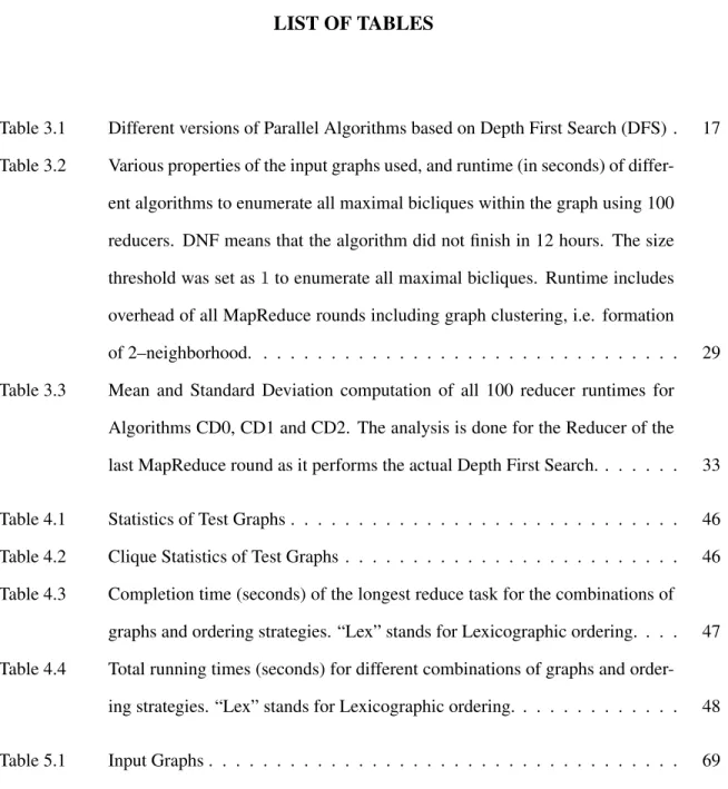
Table 3.1 Different versions of Parallel Algorithms based on Depth First Search (DFS) . 17 Table 3.2 Various properties of the input graphs used, and runtime (in seconds) of
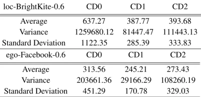
differ-ent algorithms to enumerate all maximal bicliques within the graph using 100 reducers. DNF means that the algorithm did not finish in 12 hours. The size threshold was set as1to enumerate all maximal bicliques. Runtime includes overhead of all MapReduce rounds including graph clustering, i.e. formation of 2–neighborhood. . . 29 Table 3.3 Mean and Standard Deviation computation of all 100 reducer runtimes for
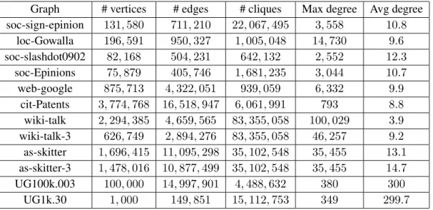
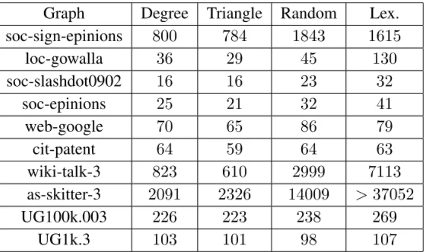
Algorithms CD0, CD1 and CD2. The analysis is done for the Reducer of the last MapReduce round as it performs the actual Depth First Search. . . 33 Table 4.1 Statistics of Test Graphs . . . 46 Table 4.2 Clique Statistics of Test Graphs . . . 46 Table 4.3 Completion time (seconds) of the longest reduce task for the combinations of
graphs and ordering strategies. “Lex” stands for Lexicographic ordering. . . . 47 Table 4.4 Total running times (seconds) for different combinations of graphs and
order-ing strategies. “Lex” stands for Lexicographic orderorder-ing. . . 48
LIST OF FIGURES
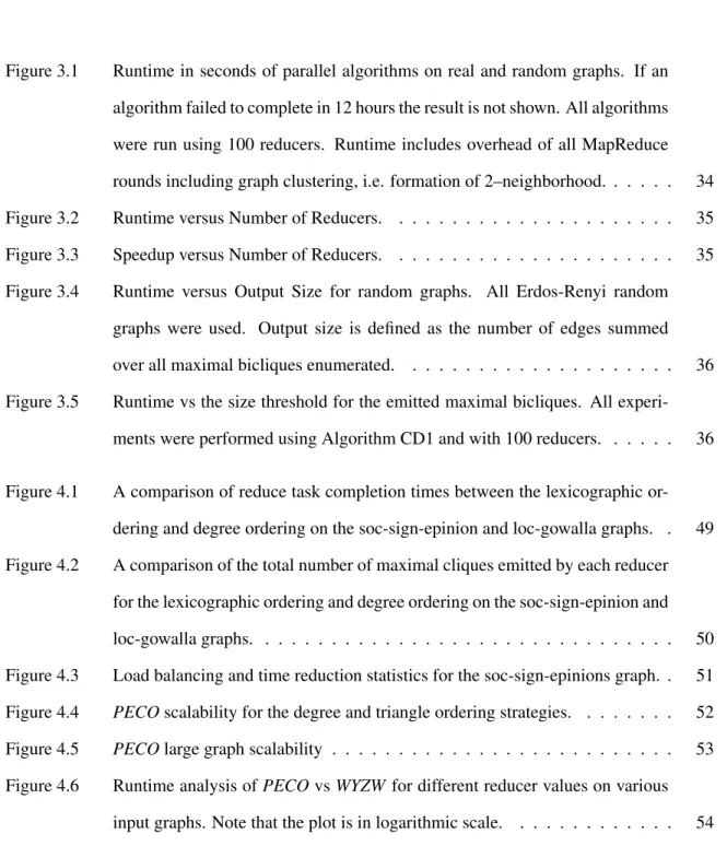
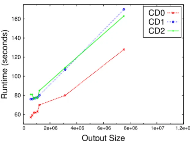
Figure 3.1 Runtime in seconds of parallel algorithms on real and random graphs. If an algorithm failed to complete in 12 hours the result is not shown. All algorithms were run using 100 reducers. Runtime includes overhead of all MapReduce rounds including graph clustering, i.e. formation of 2–neighborhood. . . 34 Figure 3.2 Runtime versus Number of Reducers. . . 35 Figure 3.3 Speedup versus Number of Reducers. . . 35 Figure 3.4 Runtime versus Output Size for random graphs. All Erdos-Renyi random
graphs were used. Output size is defined as the number of edges summed over all maximal bicliques enumerated. . . 36 Figure 3.5 Runtime vs the size threshold for the emitted maximal bicliques. All
experi-ments were performed using Algorithm CD1 and with 100 reducers. . . 36
Figure 4.1 A comparison of reduce task completion times between the lexicographic or-dering and degree oror-dering on the soc-sign-epinion and loc-gowalla graphs. . 49 Figure 4.2 A comparison of the total number of maximal cliques emitted by each reducer
for the lexicographic ordering and degree ordering on the soc-sign-epinion and loc-gowalla graphs. . . 50 Figure 4.3 Load balancing and time reduction statistics for the soc-sign-epinions graph. . 51 Figure 4.4 PECOscalability for the degree and triangle ordering strategies. . . 52 Figure 4.5 PECOlarge graph scalability . . . 53 Figure 4.6 Runtime analysis ofPECOvsWYZW for different reducer values on various
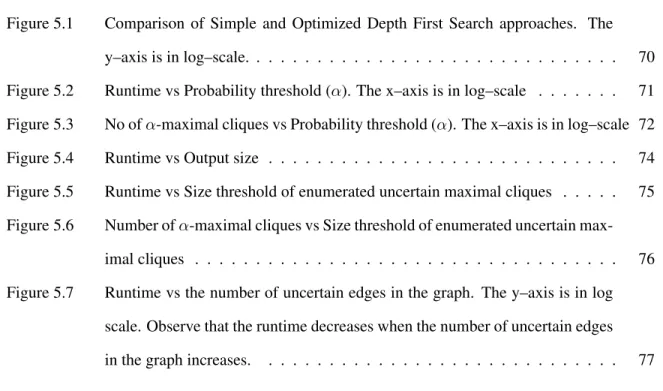
Figure 5.1 Comparison of Simple and Optimized Depth First Search approaches. The y–axis is in log–scale. . . 70 Figure 5.2 Runtime vs Probability threshold (α). The x–axis is in log–scale . . . 71 Figure 5.3 No ofα-maximal cliques vs Probability threshold (α). The x–axis is in log–scale 72 Figure 5.4 Runtime vs Output size . . . 74 Figure 5.5 Runtime vs Size threshold of enumerated uncertain maximal cliques . . . 75 Figure 5.6 Number ofα-maximal cliques vs Size threshold of enumerated uncertain
max-imal cliques . . . 76 Figure 5.7 Runtime vs the number of uncertain edges in the graph. The y–axis is in log
scale. Observe that the runtime decreases when the number of uncertain edges in the graph increases. . . 77
ACKNOWLEDGEMENTS
I would like to take a moment and thank all those whose help and support made this thesis possi-ble. First, I would like to sincerely thank Prof. Srikanta Tirthapura for his guidance and mentorship throughout my tenure as a graduate student. I have learnt a lot from him in many ways. I am much thankful to him for all his patience in all these years as I learnt my way through all my mistakes. I would also like to thank all my committee members for their help and support. I would like to thank Prof. Suraj Kothari for many helpful discussions and feedback regarding my work. I would like to thank Prof. David Fernandez-Baca with whom I had several discussions on MapReduce and also for developing my interests in algorithm design through his course. I would like to thank Prof. Chaudhuri for her support and igniting my interest in distributed systems through her course that I took. I thank Prof. Jacobson for helping me to explore Computer Security and helping me through the classes that I have taken with him. I would like to thank all Professors whose classes I have enjoyed. I would also like to thank my collaborators, Michael Svendsen and Pan Xu. I have enjoyed many fruitful discussions with both of them.
Next, I would like to thank all the good people in Iowa State University for their help and support. I must thank all the staff members in the Department of Electrical and Computer Engineering as well as in Graduate College for always answering my queries and clearing all my doubts. Special thanks goes to Vicky Thorland-Oster for giving a patient hearing all the time.
I would like to thank all my friends and neighbors in Ames, IA. Without their company, life would have been hard away from home. I can easily predict that the last five years would contribute to many of my most memorable memories.
Last, but certainly not the least, I would like to thank all my teachers from South Point High School who shaped me in my formative years and helped me to develop my interest in science. I will be indebted to them all my life for teaching me to always think logically, keep an open mind and helping me to grow my “Courage to Know”!
ABSTRACT
Graphs represent relationships. Some relationships can be represented as a deterministic graph while others can only be represented by using probabilities. Mining dense structures from graphs help us to find useful patterns in these relationships having applications in wide areas like social network analysis, bioinformatics etc. Arguably the two most fundamental dense substructures are Maximal Cliques and Maximal Bicliques. The enumeration of both these structures are central to many data mining problems. With the advent of “big data”, real world graphs have become massive. Recently systems like MapReduce have evolved to process such large data. However using these systems to mine dense substrucures in massive graphs is an open question. In this thesis, we present novel parallel algorithms using MapReduce for the enumeration of Maximal Cliques / Bicliques in large graphs. We show that our algorithms are work optimal and load balanced. Further, we present a detailed evaluation which shows that the algorithm scales to large graphs with millions of edges and tens of millions of output structures. Finally we consider the problem of Maximal Clique Enumeration in an Uncertain Graph, which is a probability distribution on a set of deterministic graphs. We define the notion of a maximal clique for an uncertain graph, give matching upper and lower bounds on the number of such structures and present a near optimal algorithm to mine all maximal cliques.
DECLARATION
Publications The work presented in this thesis has been published in the following conference proceedings and journals:
• The content of Chapter 3 has been published in Arko Provo Mukherjee and Srikanta Tirthapura, Enumerating maximal bicliques from a large graph using mapreduce, In Proceedings IEEE 3rd International Congress on Big Data (2014). For details see Mukherjee and Tirthapura (2014).
• The content of Chapter 4 has been published in Michael Svendsen, Arko Provo Mukherjee and Srikanta Tirthapura, Mining maximal cliques from a large graph using mapreduce: Tackling highly uneven subproblem sizes, Journal of Parallel and Distributed Computing, Special Issue: Scalable Systems for Big Data Management and Analytics (2014). For details see Svendsen et al. (2014).
• The content of Chapter 5 has been published in Arko Provo Mukherjee, Pan Xu and Srikanta Tirthapura, Mining maximal cliques from an uncertain graph, In Proceedings IEEE 31st Inter-national Conference on Data Engineering (2015). For details see Mukherjee et al. (2015).
My contributions This thesis is a result of work done in collaboration with my advisor Prof. Srikanta Tirthapura as well as Michael Svendsen and Dr. Pan Xu. My contributions are as follows:
• Parallel Algorithm design to enumerate all maximal bicliques from a large graph. This was done using Hadoop. We show that the algorithms presented are work optimal and are scalable to a high degree of parallelism. The results were published in Mukherjee and Tirthapura (2014). I worked on the design, analysis, implementation as well as experiments on this project under the guidance of my advisor Prof. Tirthapura.
• Comparitive analysis of Algorithms for maximal clique enumeration with MapReduce. I helped in performing comparitive analysis of algorithm due to the masters thesis of Michael Svendsen
(see Svendsen (2012)) with the previous state of the art for this problem. I also contributed in tuning the implemetations for faster runtime and participated in the discussion of this project. All results were published in Svendsen et al. (2014). Note: Parts of this Chapter is from Master Thesis Svendsen (2012) and hence there is significant overlap between the same. My contribution to this Chapter is primarily the comparitive analysis fo the Algorithms and the rest of the material is provided for the purpose of clarity.
• Defining the problem of maximal clique enumeration for an uncertain graph. The bound on the number of structures was done in collaboration with Dr. Pan Xu and Prof. Srikanta Tirthapura. The design and analysis of the Algorithm was done under the guidance of Prof. Tirthapura. I also implemented the Algorithm and performed experiments to validate our theoretical analysis. This work was published in Mukherjee et al. (2015).
CHAPTER 1. INTRODUCTION
1.1 Motivation
A graph (or network) is a natural abstraction to model rich relationships in data, and massive graphs are ubiquitous in applications such as online social networks Mislove et al. (2007); Newman et al. (2002), information retrieval from the web Broder et al. (2000), citation networks An et al. (2004), and physical simulation and modeling Wodo et al. (2012), to name a few. Finding information from such data can often be reduced to a problem of mining features from massive graphs.
Working with large graphs presents many challenges. A large graph does not always fit in the memory of a single computer. Hence such a graph must be stored in a distributed fashion among multiple nodes of a cluster. Further, since the entire graph is not available on a single node in the cluster, any algorithm that uses the graph as an input does not have the luxury of having the entire input on every node. Each computer has to work only with a subset of the entire graph to produce the results. This means that large graphs need to be processed on multiple processors in parallel. In many other cases, we can construct such a large graph only with certain probability as all information about the large cannot be obtained. An example of such a massive graph can be the telecommunication network, where we can assume a link (edge) only with a certain probability Ghosh et al. (2007).
Mining patterns from such large graph is an important topic in today. As mentioned above graphs represent many real life scenarios. Pattern mining in a graph help us to find interesting relationships in all the different scenarios that a graph can represent. Many a times finding dense regions in the network can help us find interesting relationships. Dense connections imply that those regions in the graph are closely connected to each other and hence form strong relationships. Thus mining dense substructures such as cliques, quasi-cliques, bicliques, quasi-bicliques etc. is an important area of study Alexe et al. (2004); Gibson et al. (2005); Abello et al. (2002); Sim et al. (2006). Many different dense substructures
have been defined and studied Lee et al. (2010). We concentrate on arguably the two most fundamental dense substructures that can be found in a graph, maximal clique and maximal biclique and then focus on the problems of mining maximal cliques and maximal bicliques. We call these problems as the Maximal Clique Enumeration (MCE) and Maximal Biclique enumeration (MBE).
Many graph mining tasks have relied on enumerating maximal cliques and bicliques to identify sig-nificant substructures within the graph. For instance, maximal clique enumeration is used in clustering and community detection in social and biological networks Palla et al. (2005), in the study of the co-expression of genes under stress Rokhlenko et al. (2007), in integrating different types of genome map-ping data Harley and Bonner (2001), and other applications in bio-informatics and data mining Chen and Crippen (2005); Grindley et al. (1993); Jonsson and Bates (2006); Mohseni-Zadeh et al. (2004); Zhang et al. (2008a); Hattori et al. (2003); Zaki et al. (1997). Similarly enumerating maximal bicliques has been used to identify significant substructures within the graph. For instance the analysis of web search queries Yi and Maghoul (2009) considered the “click-through” graph, where there are two types of vertices, web search queries and web pages. There is an edge from a search query to every page that a user has clicked in response to the search query. MBE was used in clustering queries using the click through graph. MBE has been used in social network analysis, in detection of communities in social networks Lehmann et al. (2008), and in finding antagonistic communities in trust-distrust networks Lo et al. (2011). It has also been applied in detecting communities in the web graph Kumar et al. (1999); Rome and Haralick (2005). In bioinformatics, MBE has been used widely e.g. in construction of the phylogenetic tree of life Driskell et al. (2004); Sanderson et al. (2003); Yan et al. (2005); Nagarajan and Kingsford (2008), structure discovery and analysis of protein-protein interaction networks Bu et al. (2003); Schweiger et al. (2011), analysis of gene-phenotype relationships Xiang et al. (2012), prediction of miRNA regulatory modules Yoon and Micheli (2005), modeling of hot spots at protein interfaces Li and Liu (2009), and in analysis of relationships between genotypes, lifestyles, and diseases Mushlin et al. (2007). Other applications include Learning Context Free Grammars Yoshinaka (2011), finding correlations in databases Jermaine (2005), for data compression Agarwal et al. (1994), role mining in role based access control Colantonio et al. (2010), and process operation scheduling Mouret et al. (2011).
While it is easy to find a single maximal clique / biclique in a graph, enumerating all maximal cliques / bicliques are an NP-hard problems Valiant (1979); Peeters (2003). This does not however mean that typical cases are unsolvable. In fact, there are output-polynomial time algorithms for both these problems, whose theoretical runtime is bounded by a polynomial in the number of vertices in the graph, and the number of structures that are output Tsukiyama et al. (1977); Alexe et al. (2004). Thus it is reasonable to expect to be able to devise algorithms for MBE that work on large graphs, as long as the number of maximal bicliques output is not too high.
However, current methods for enumerating cliques / bicliques have the following drawbacks. Most methods are sequential algorithms that are unable to make use of the power of multiple processors. For handling large graphs, it is imperative to have methods that can process a graph in parallel. Next, they have been evaluated only on small graphs of a few thousands of vertices and a few hundred thousand maximal bicliques, and have not been shown to scale to large graphs. For instance, the popular “con-sensus” method for biclique enumeration Alexe et al. (2004) presents experimental data only on graphs of up to 2,000 vertices, and about 140,000 maximal bicliques, and other works Li et al. (2007); Liu et al. (2006) are also similar. Further little is know as to how to enumerate these structures for an Uncertain Graph. In this work we propose to solve some of these fundamental problems for large deterministic and uncertain graphs.
1.1.1 Big Data Software Tools
Recently parallel programming platforms have evolved that simplifies parallel programming. In this section we discuss a few such parallel programming frameworks. RecentlyMapReduceDean and Ghemawat (2004, 2008); Karloff et al. (2010) has become a popular platform for parallel programming. The MapReduce programming model was designed to address a common problem with parallel pro-gramming and algorithm design. It was observed by the authors of the model that many of the problems that need to be solved with a parallel algorithm due to the size of the input are actually simple. However, the design and implementation of the parallel solution can quickly become very complex when trying to write parallel programs that can run on many nodes. The MapReduce model was developed to address just that.
The model is inspired by the mapandreduceprimitives from functional programming languages like Lisp. The algorithm design must be split up into one / multiple rounds of MapReduce. Each round must have amap and areducemethod. Effectively the entire algorithm is broken down into a series of map and reduce methods. The input to the program is processed by the map method and it emits a sequence of key / value pairs< K, V >. Then the system groups the values according to the keys and sorts them. Thus for each keyki ⊂K, the system generates< ki, list(Vi)>. This is then passed on to the reduce methods as their input which will then process them as per the algorithm. The output from thereducemethods can then be used as the input to the next round.
The reason for the success of MapReduce is its relative simplicity with respect to many other popu-lar parallel programming platforms. All the designer needs to do is to think and implement the solution to the problem as a sequence of map and reduce primitives. The system automatically breaks up the input into slices and feeds them into the map method. It also takes care of interprocess communication, load balancing, fault tolerance and data locality. All these complexities are hidden from the program-mer. The MapReduce framework uses an underlying distributed file system known as the Google File System Ghemawat et al. (2003) which takes care of distributing the data and maintaining multiple replica of the data to make the system more robust and fault tolerant. The other important benefit of the MapReduce model is that it can be implemented on relatively inexpensive commodity clusters made of low cost commodity hardware. MapReduce assumes serial communication network like the Ethernet and hence no sophisticated parallel communication network is required. This helps in lowering the hardware cost considerably.
The original MapReduce implementation by Google is not publicly available for use or distribu-tion. Hence, for this work, we use the popular Open Source implementation of MapReduce known as Hadoop White (2009). Hadoop is a JAVA implementation of the MapReduce programming model and provides a JAVA API. It also provides bindings to different other programming languages like C++, Python etc. Additionally it replaces the Google File system with its own implementation of a Distributed File System called HDFS Shvachko et al. (2010).
All these benefits come with few drawbacks — firstly the user is forced to think in the restrictive model of Map and Reduce. Every algorithm may not be naturally expressible in terms of MapReduce. This makes it difficult to express all algorithms in terms of map and reduce methods. Secondly, it is a
batch processing system with low response time. Also, it is hard to do dynamic load balancing of the input graph.
While we evaluated an implementation on top of MapReduce, the ideas in this work are more generally applicable and can easily be adapted to other frameworks such as Pregel Malewicz et al. (2010) and Spark Zaharia et al. (2012).
1.1.2 Uncertain Graph Model
Large datasets often contain information that is uncertain in nature. For example, given people A and B, a question of the form “does A know B” may not be definitively answered using available information. In such a case, it is a common solution to use probability to quantify our confidence in this relation, and say that the relation exists with a probability ofp, for some valuepdetermined from the available information. Such uncertain graphs have often been used in modeling real data, for ex-ample, various communication networks Ghosh et al. (2007); Biswas and Morris (2005); Kawahigashi et al. (2005), in social networks Adar and Re (2007); Guha et al. (2004); Kempe et al. (2003); Liben-Nowell and Kleinberg (2003); Kuter and Golbeck (2010), protecting privacy while modeling social networks Boldi et al. (2012), protein interaction networks Asthana et al. (2004); Bader et al. (2004); Rhodes et al. (2005), analyzing regulatory networks in biological systems Jiang et al. (2006) and min-ing information from biological databases Sevon et al. (2006). While the notion of a maximal cliques or bicliques are well understood in a deterministic graph, it is not well defined or understood within an uncertain graph.
1.2 Literature review
1.2.1 Maximal Cliques
We first discuss related work on sequential MCE and then on parallel MCE. An early work due to Bron and Kerbosch (1973) is an algorithm based on depth-first-search with good experimental per-formance on typical inputs, but whose worst case behavior is poor. Other algorithms stemming from this work include Tomita et al. (2006). Another branch of enumeration algorithms provide output sen-sitive runtime guarantees, i.e. the runtime is proportional to the size of the output. These algorithms
stem from the Tsukiyama et al. (1977) algorithm, which has a running time ofO(|V||E|µ), whereµis the number of maximal cliques. However, these output sensitive algorithms tend not to perform as well as the worst case optimal algorithms in practice Tomita et al. (2006); Eppstein et al. (2010).
Early works in the area of parallel MCE include Zhang et al. (2005) and Du et al. (2006). Zhanget al.developed an algorithm based on the Kose et al. (2001) algorithm. Since these algorithms are based on breadth first search, they are able to enumerate maximal cliques in increasing order of size, but this makes the memory requirements very large. Du et al. (2006), present a parallel algorithm based on the output-sensitive class of algorithms. However, as also noted by Schmidt et al. (2009), this algorithm suffers from poor load balance; the graphs addressed by these experiments are quite small, they have about 150,000 maximal cliques and a million edges.
Schmidt et al. (2009) identify load balancing as a significant issue in parallel MCE and present a parallel algorithm that uses “work stealing” to dynamically distribute load among processors. Their algorithm is designed for use with MPI, where the user can control the actions of a process and the manner of parallelism to a high degree of detail, when compared with MapReduce. In their algorithm, processes explore tasks in parallel until they run out of work, at which point idle processes request for more work from busy processes (work stealing). This continues until all processes are idle. Such types of work stealing and dynamic load balancing are expensive to implement in the MapReduce model, since the processes are synchronized at each stage of Map and Reduce – for instance, all mappers need to complete before reducers start processing data. Our algorithm also implements effective load balancing, but in a more pre-determined and static manner.
Wu et al. (2009) present an MCE algorithm designed for MapReduce. The algorithm splits the input graph into many subgraphs, which are then independently processed to enumerate cliques. However this work does not address load balancing, and in addition, their algorithm may enumerate non-maximal cliques, so that an additional post-processing step is needed to only emit maximal cliques.
dMaximalCliques Lu et al. (2010) is another parallel MCE algorithm, based on the sequential algo-rithm of Tomita et al. (2006). This algoalgo-rithm works in two phases. The first phase enumerates maximal, duplicate, and maximal cliques, and the second post-processing phase removes duplicate and non-maximal cliques from the output. However, this post-processing phase can be very expensive since the output prior to filtering can become much larger than the final output; for instance, on the wikitalk-3
graph the first enumeration phase takes 7 minutes (on 20 processors), and the second post-processing phase takes 228 minutes (on 80 processors). The algorithm is implemented for the Sector/Sphere Gu and Grossman (2009) framework.
1.2.2 Maximal Bicliques
Some previous work related to MBE are as follows. Makino and Uno (2004) describes methods to enumerate all maximal bicliques in abipartite graph, with the delay between outputting two bicliques bounded by a polynomial in the maximum degree of the graph. Zhang et al. (2008b) describe a branch-and-bound algorithm for the same problem. However, these approaches do not work for general graphs, as we consider here.
There is a variant of MBE where we only seekinducedmaximal bicliques in a graph. An induced maximal biclique is a maximal biclique which is also an induced subgraph; i.e. a maximal biclique
hL, Ri in graphGis an induced maximal biclique if LandR are themselves independent sets inG. We consider thenon-inducedversion, where edges are allowed in the graph between two vertices that are both inL, or both inR(such edges are of course, not a part of the biclique). The set of maximal bicliques that we output will also contain the set of induced maximal bicliques, which can be obtained by post-processing the output of our algorithm. Note that for a bipartite graph, every maximal biclique is also an induced maximal biclique. Algorithms for Induced MBE include work by Eppstein (1994), Dias et al. (2005), and Gaspers et al. (2008).
Alexe et al. (2004) present an iterative algorithm for non-induced MBE using the “consensus” method. Another technique for MBE is based on a recursive depth first search (DFS) Li et al. (2007); Liu et al. (2006). Li et al. (2007) presents an approach based on a connection with mining closed pat-terns in a transactional database, and apply the algorithm from Uno et al. (2004), which is based on depth first search. Liu et al. (2006) present a more direct algorithm for biclique enumeration based on depth first search.
Another approach to MBE is through a reduction to the problem of enumerating maximal cliques, as described by G´ely et al. (2009). Given a graphGon which we need to enumerate maximal bicliques, a new graphG0 is derived such that through enumerating maximal cliques inG0 using an algorithm such as Tomita et al. (2006); Tsukiyama et al. (1977), it is possible to derive the maximal bicliques in
G. However, this approach is not practical for large graphs since in going fromGtoG0, the number of edges in the graph increases significantly.
To our knowledge, the only prior work on parallel algorithms for MBE is by Nataraj and Selvan (2009), who use the correspondence between maximal bicliques and closed patterns Li et al. (2007) to derive a parallel method for enumerating maximal bicliques. A significant issue is that Nataraj and Selvan (2009) assumes that the input graph is presented as an adjacency matrix, which is then converted into a transactional database and distributed among the processors. In contrast, we do not assume an adjacency matrix, but assume that the graph is presented as a list of edges. Thus we are able to work on much larger graphs than Nataraj and Selvan (2009); the largest graph that they consider has 500 vertices and about 9000 edges.
1.2.3 Uncertain Graphs
There has been recent work in the database community on various problem on uncertain graphs, including probability-threshold based shortest paths Yuan et al. (2010), nearest neighbors Potamias et al. (2010), enumerating frequent and reliable subgraphs Hintsanen and Toivonen (2008); Zou et al. (2010c); Jin et al. (2011a); Zou et al. (2010a); Liu et al. (2012); Kollios et al. (2013), distance-constrained reachability Jin et al. (2011b). Note that our problem is different from the problems mentioned above. For example, finding reliable subgraphs problem is to find all subgraphs of the uncertain graph such which are connected with a high probability. However, these individual subgraphs may be sparse. We are interested instead in finding dense subgraphs whose probability of existence is greater than a given threshold.
There is relatively little known about mining dense substructures from an uncertain graph. To our knowledge, the only previous work on mining maximal cliques in an uncertain graph is by Zou et al. (2010b). Our work is different from theirs in significant ways. Mainly, while we focus on enumerating allα-maximal cliques in a graph, they focus on a different problem, that of enumerating thekmaximal cliques with the highest probability of existence. We present bounds on the number of such cliques that could exist, while by definition, their algorithm outputskcliques.
1.3 Contributions
The following are the contributions of this work.
• We present a generic parallel solution for MCE / MBE using the MapReduce framework Dean and Ghemawat (2008). At a high level, our approach clusters the input graph into overlapping subgraphs that can be processed independently in parallel, by different reducers.
• Applying the generic framework to solve MBE using MapReduce
• Designing optimizations helping in reducing the overlap in the work done by different subtasks. It is usually not possible to assign disjoint subgraphs to different processors, and the subgraphs assigned to different tasks will overlap, sometimes significantly. Through a careful partitioning of the search space among the different tasks, we reduce redundant work among the tasks (this partitioning depends on details of the sequential algorithm used at each task).
• Designing load balancing strategies for Maximal Biclique problem. With a graph analysis task such as biclique enumeration, the complexity of different subgraphs varies significantly, depend-ing on the density of edges in the subgraph. Naively done, this can lead to a case where most reducers finish quickly, while only a few take a long time, leading to a poor parallel performance. We present a solution to keep the load more balanced, based on an ordering of vertices, which reduces enumeration load on subgraphs that are dense, and increases the load on subgraphs that are sparse, leading to a better parallel efficiency.
• A direct parallelization of the consensus sequential algorithm Alexe et al. (2004), using an ap-proach different from clustering. We found that while this apap-proach may use a smaller memory per node that the clustering approach, it requires substantially greater runtime.
• An experimental evaluation of the state of the art Maximal Clique Enumeration Algorithm on top of MapReduce from Svendsen (2012) with previous work. The result of the evaluation clearly demonstrates that the Algorithm described in Svendsen (2012) outperforms the previous MCE Algorithm for MapReduce.
• We consider a basic question on maximal cliques within uncertain graphs:how manyα-maximal
cliques can be present within an uncertain graph? For the case of deterministic graphs, this
question was first considered by Moon and Moser (1965) in 1965, who presented matching upper and lower bounds for the largest number of maximal cliques within a graph; on a graph withn
vertices, the largest possible number of maximal cliques is3n31. For the case of uncertain graphs,
we present the first matching upper and lower bounds for the largest number ofα-maximal cliques in a graph onn vertices. We show that for0 < α < 1, the maximum number of α-maximal cliques in an uncertain graph is bn/n2c
, i.e. there is an uncertain graph onnvertices with bn/n2c
uncertain maximal cliques and no uncertain graph onnvertices can have more than bn/n2c α -maximal cliques.
• We present a branch-and-bound based algorithm for enumerating allα-maximal cliques within an uncertain graph. We prove that the algorithm enumerates everyα-maximal clique in the graph and provide an upper bound on the runtime. Our experimental analysis on synthetic and real-world graphs show that the algorithm can enumerate maximal cliques in an uncertain graph of tens of thousands of vertices, over hundred thousand edges and over two million α-maximal cliques. Interestingly, the observed runtime of this algorithm is proportional to the size of the output, i.e. the number ofα-maximal cliques that are present in the graph.
• Application of the generic framework to MCE and comparison with previous work.
• Experimental validations for all the contributions stated above.
1
CHAPTER 2. PRELIMINARIES
In this Chapter we discuss some definitions and observations that we use throughout this thesis. We consider a simple undirected graphG = (V, E)without self-loops or multiple edges, whereV is the set of all vertices and E is the set of all edges of the graph. Letn = |V|andm = |E|. Graph
H= (V1, E1)is said to be a sub-graph of graphG= (V, E)ifV1⊂V andE1 ⊂E.His known as an
induced subgraph ifE1consists of all edges ofGthat connect two vertices inV1. For vertexu∈V, let η(u)denote the vertices adjacent tou. For a set of verticesU ⊆V, letη(U) = S
u∈U
η(u). For vertex
u ∈ V andk > 0, letηk(u) denote all vertices that can be reached fromu inkhops. ForU ⊆ V, letηk(U) = S
u∈U
ηk(u). We callηk(U)as thek-neighborhood ofU. For a set of verticesU ⊆V, let
Γ(U) = T
u∈U η(u).
An uncertain graph is a probability distribution over a set of deterministic graphs. Formally, an uncertain graph is a tripleG = (V, E, p), whereV is a set of vertices, E ⊆V ×V is a set of edges, andp : E → (0,1]is the probability function that assigns a probabilityp(e) to each edgee ∈E. As in prior work on uncertain graphs, we assume the probabilities assigned to different edges are mutually independent.
Definition 1. A set of verticesC ⊆V is a clique in a graphG= (V, E), if every pair of vertices inC are connected by an edge inE.
Definition 2. A set of verticesM ⊆V is a maximal clique in a GraphG= (V, E), if (1)M is a clique inGand (2) There is no vertexv ∈V \Msuch thatM∪ {v}is a clique inG.
Definition 3. AbicliqueB =hL, Riis a subgraph ofGcontaining two non-empty and disjoint vertex sets,LandRsuch that for any two verticesu∈Landv ∈R, there is an edge(u, v)∈E.
Note that the definition on B = hL, Ridoes not impose any restriction on the existence of edges among the vertices withinRor withinL, i.e., we considernon-inducedbicliques.
Definition 4. A bicliqueM =hL, RiinGis said to be a maximal biclique if there is no other biclique M0=hL0, R0i 6=hL, Risuch thatL⊂L0andR⊂R0.
TheMaximal Clique Enumeration Problem (MCE)is to enumerate the set of all maximal cliques in graphG= (V, E).
The Maximal Biclique Enumeration Problem (MBE) is to enumerate the set of all maximal bicliques in graphG= (V, E).
Definition 5. In an uncertain graphG, for a set of verticesC⊆V, the clique probability ofC, denoted byclq(C,G), is defined as the probability that in a graph sampled fromG,Cis a clique. For parameter 0≤α≤1,Cis called anα-clique ifclq(C,G)≥α.
For any set of verticesC ⊆V, letECdenote the set of edges{e= (u, v)|e∈E, u, v∈Candu6= v}, i.e. the set of edges ifCwere a clique.
Observation 1. For any set of verticesC⊆V,clq(C,G) =Q
e∈ECp(e)
Proof. LetGbe a graph sampled fromG. The setCwill be a clique inGiff every edge inECis sampled intoG. Since the probability of selecting different edges is independent, the observation follows. Definition 6. Given an uncertain graphG = (V, E, p), and a parameter0 ≤α ≤1, a setM ⊆V is defined as anα-maximal clique if (1)M is anα-clique inG, and (2) There is no vertexv ∈(V \M) such thatM ∪ {v}is anα-clique inG.
Definition 7. TheMaximal Clique Enumeration problem in an Uncertain GraphG is to enumerate all vertex setsM ⊆V such thatM is anα-maximal clique inG.
The following two observations follow directly from Observation 1.
Observation 2. For any two cliquesAandBinG, ifB⊂Athen,clq(B,G)≥clq(A,G).
Observation 3. LetCbe anα-clique inG. Then for alle∈ECwe havep(e)≥α.
From the above observation, it is clear that we can drop all edges esuch thatp(e) < α, prior to enumeratingα-maximal cliques inG.
CHAPTER 3. MINING ALL MAXIMAL BICLIQUES
3.1 Sequential Algorithms
We describe the two general approaches to sequential algorithms for MBE that we consider, one based on depth first search (see Liu et al. (2006)) and another based on a “consensus algorithm” (see Alexe et al. (2004)).
3.1.0.1 Sequential DFS Algorithm
The basic sequential depth first approach (DFS) that we use is described in Algorithm 1, based on work by Liu et al. (2006). It attempts to expand an existing maximal biclique into a larger one by including additional vertices that qualify, and declares a biclique as maximal if it cannot be expanded any further. The algorithm takes the following inputs: (1) the graphG= (V, E), (2) the current vertex set being processed,X, (3)T, the tail vertices ofX, i.e. all vertices that come afterXin lexicographical ordering and (4)s, the minimum size threshold below which a maximal biclique is not enumerated. s
can be set to1so as to enumerate all maximal bicliques in the input graph. However, we can setsto a larger value to enumerate only large maximal bicliques such that forB =hL, Ri, we have|L| ≥ s
and|R| ≥s. The size thresholdsis provided as user input. The other inputs are initialized as follows:
X=∅,T =V.
The algorithm recursively searches for maximal bicliques. It increases the size of X by recur-sively adding vertices from the tail set T, and pruning away those vertices fromT which cannot be added toX to expand the biclique. From the expandedX, the algorithm outputs the maximal biclique
Algorithm 1:MineLMBC(G,X,T,s)
1 forall thevertexv∈T do 2 if|Γ(X∪ {v})|< sthen 3 T ←T\ {v};
4 if|X|+|T|< sthen 5 return
6 Sort vertices inT as per ascending order of|η(X∪ {v})|; 7 forall thevertexv∈T do
8 T ←T\ {v}; 9 if|X∪ {v}|+|T| ≥sthen 10 N ←Γ(X∪ {v}); 11 Y ←Γ(N); 12 BicliqueB ← hY, Ni; 13 if(Y \(X∪ {v}))⊆Tthen 14 if|Y| ≥sthen
15 EmitBas a maximal biclique ; 16 MineLMBC(G,Y,T\Y,s) ;
3.1.0.2 Consensus Algorithm
Alexe et al. (2004) present an iterative approach to MBE. This algorithm starts off with a set of sim-ple “seed” bicliques. In each iteration, it performs a “consensus” operation, which involves performing a cross-product on the set of current candidates bicliques with the seed bicliques, to generate a new set of candidates, and the process continues until the set of candidates does not change anymore. After each stage, the newly found bicliques can be expanded to find new maximal bicliques. After each step, the duplicate maximal bicliques can be dropped. It is proved that these algorithms exactly enumerate the set of maximal bicliques in the input graph. Algorithm 2 shows the sequential consensus Algorithm. For further details, we refer the reader to Alexe et al. (2004).
The consensus approach has a good theoretical guarantee, since its runtime depends on the number of maximal cliques that are output. In particular, the runtime of the MICA version of the algorithm is proved to be bounded byO n3·N
wherenis the number of vertices andNtotal number of maximal bicliques inG. The consensus algorithm has been found to be adequate for many applications and is quite popular.
Algorithm 2:Sequential Consensus Algorithm
1 Load GraphG= (V, E);
2 R ←Collection of all Stars inG// Biclique formed by a vertex and its neighbors
3 S ←∅;
4 forall theb∈Rdo 5 m←Extendb; 6 S←S∪m;
7 O ←S;// Add seed set to the output
8 P ←S;// Initialize set PREV with SEED
9 repeat
10 T ←Consensus between all maximal bicliques inSandP ;
11 C←∅;
12 forall theb∈T do
13 m←Extend bicliqueb;
14 ifmis not a duplicatethen
15 C←C∪m;
16 O←O∪C;
17 P ←C;
18 untilN is Empty;
3.2 Parallel Algorithms for MBE
We describe our parallel algorithms for MBE, and give an outline of how these are implemented using MapReduce. We first present a basic clustering approach,which can be used with any sequential algorithm for MBE, followed by enhancements to the basic clustering approach.
3.2.1 Basic Clustering Approach
For eachv ∈V, let subgraph (cluster)C(v)be defined as the induced subgraph on all vertices in
η2(v)(the 2-neighborhood ofvinG). We first note the following.
Lemma 1. Each maximal bicliqueB inG= (V, E)is a maximal biclique inC(v)for every vertexv inB. Further, for anyv∈V, each maximal biclique inC(v)is also a maximal biclique inG.
Proof. We first prove the first direction, i.e. each maximal bicliqueB inG = (V, E) is a maximal biclique inC(v)for every vertexv that is contained inB. Consider a maximal bicliqueM =hL, Ri
biclique, for eachu∈R,uis a neighbor ofv. Similarly, every vertexw∈Lis a neighbor ofv, and is hence inη2(v). HenceM is completely contained inC(v). Note thatM is also a maximal biclique in C(v). To see this, note that ifM is not maximal biclique inC(v), thenM is not maximal inGeither.
Next we prove the other direction, that is we prove that every maximal biclique in each cluster
C(v)is also a maximal biclique inG. Consider a maximal bicliqueM =hL, Ricontained in cluster
C(v). We prove by contradiction. We assumeMis non–maximal inG. This implies that there exists a maximal bicliqueM0 =hL0, R0iinGsuch thatM is completely contained inM0. LetMˆ ={L∪R}
andMˆ0 = {L0 ∪R0}. Let us consider a vertexa ∈ {Mˆ0\Mˆ}. As per our assumption,a 6∈ C(v).
Also, without loss in generality, assumev ∈L. There are two cases that are possible. Eithera∈Ror
a ∈ L. Let us first consider the first case, i.e. vertexa ∈ R. Now vertexaextendsM = hL, Riby adding vertexatoR. This means ais connected to each vertexu ∈ L. Remember thatv ∈L. Fora
to extendR, vertexamust be connected to all vertices inL. This implies that vertexais connected to vertexvby edge(v, a). This is a contradiction asa6∈C(v). Thus no vertexa6∈C(v)can extendR. Let us now take the other case, i.e. a∈L. This implies that there exists an edge(a, b)between vertex
aand any vertexb ∈η(v), i.e. a∈η2(v). Again, this is a contradiction asa6∈ C(v). Thus no vertex
a6∈C(v)can extendL.
3.2.2 Algorithm CDFS – Suppressing Duplicates
With the above observation, a basic parallel algorithm for MBE first constructs the different clusters
{C(v)|v ∈ V}, and then enumerates the maximal bicliques in the different clusters in parallel, using any sequential algorithm for MBE for enumerating the bicliques within each cluster.
While each maximal biclique inGis indeed enumerated by the above approach, the same biclique may be enumerated multiple times. To suppress duplicates, the following strategy is used: a maximal bicliqueB arising from clusterC(v) is emitted only if v is the smallest vertex in B according to a lexicographic total order on the vertices. The basic clustering framework is generic and can be used with any sequential algorithm for MBE. We have used a variant of the DFS-based sequential algorithm due to Liu et al. (2006), as well as the sequential consensus algorithm due to Alexe et al. (2004). We call the above basic clustering algorithm using DFS-based sequential algorithm as “CDFS”.
Observation 4. Algorithm CDFS enumerates every maximal biclique in graphG = (V, E) exactly once.
There are two significant problems with the CDFS algorithm described above. First isredundant work. Although each maximal biclique inGis emitted only once, through suppressing duplicate output, it will still be generated multiple times, in different clusters. This redundant work significantly adds to the runtime of the algorithm. Second is anuneven distribution of load among different subproblems. The load on subproblemC(v)depends on two factors, the complexity of clusterC(v)(i.e. the number and size of maximal bicliques withinC(v)) and the position ofvin the total order of the vertices. The earliervappears in the total order, the greater is the likelihood that a maximum biclique inC(v)hasv
has its smallest vertex, and hence the greater is the responsibility for emitting bicliques that are maximal withinC(v). A lexicographic ordering of the vertices will lead to a significantly increased workload for clustersC(v)wherevappears early in the total order and a correspondingly low workload for clusters
C(v)wherevoccurs earlier in the total order.
Table 3.1: Different versions of Parallel Algorithms based on Depth First Search (DFS)
Label Algorithm
CDFS Clustering based on Depth First Search (DFS) CD0 CDFS + Reducing Redundant Work, without Load Balancing CD1 CDFS + Reducing Redundant Work + Load Balancing using Degree
CD2 CDFS + Reducing Redundant Work + Load Balancing using Size of 2-neighborhood
3.2.3 Algorithm CD0 – Reducing Redundant Work
In order to reduce redundant work done at different clusters, we begin with the basic clustering approach and modify the sequential DFS algorithm for MBE that is executed at each reducer. We first observe that in clusterC(v), the only maximal bicliques that matter are those with v as the smallest vertex; the remaining maximal bicliques inC(v)will not be emitted by this reducer, and need not be searched for here. We use this to prune the search space of the sequential DFS algorithm used at the reducer. The algorithm at the reducer is presented in Algorithms 7 and 8.
The above algorithm, the “optimized DFS clustering algorithm”, or “CD0” for short, is described in Algorithm 3. This takes two rounds of MapReduce. The first round, described in Algorithms 4
(map) and 5 (reduce), is responsible for generating the 1-neighborhood for each vertex. The second round, described in Algorithms 6 (map) and 7 (reduce) first constructs the clustersC(v)and runs the optimized sequential DFS algorithm at the reducer to enumerate local maximal bicliques. We assume that the graph is presented as a file in HDFS organized as a list of edges with each line in the file containing one edge.
All search paths in the algorithm which lead to a maximal biclique having a vertex less thanvcan be safely pruned away. Hence, before starting the DFS, we prune away all vertices in the Tail set that are less thanv, as described in Algorithm 7. Also, in DFS Algorithm 8, we prune the search path in Line 12 if the generated neighborhood contains a vertex less thanv– maximal bicliques along this search path will not havevas the smallest vertex. Finally in Line 19 of Algorithm 8, we emit a maximal biclique only if the smallest vertex is the same as the key of the reducer in Algorithm 7.
Algorithm 3:Algorithm CD0 Input: Edge List ofG= (V, E)
1 MapReduce Round One (Map) – Algorithm 4 ; 2 MapReduce Round One (Reduce) – Algorithm 5 ;
3 MapReduce Round Two (Map) – Algorithm 6 ;
4 MapReduce Round Two (Reduce) – DFS – Algorithm 7 ;
Algorithm 4:Algorithm CD0 Round One – Map Input: Edge(x, y)
1 // Generate Adjacency List for vertices x and y
2 Emit (key←x,value←y) ; 3 Emit (key←y,value←x) ;
Algorithm 5:Algorithm CD0 Round One – Reduce Input: key=v,value={v1, v2,· · · , vd}
1 // Generate Adjacency List for vertex v
2 N ←∅;
3 forall theval∈valuedo 4 N ←N ∪val;
5 // Add the neighbors of key to N
Algorithm 6:Algorithm CD0 Round Two – Map Input:key=v,value=N
1 // Create Two Neighborhood for vertex v
2 Emit (key←v,value←N) ; 3 forall they∈N do
4 Emit (key←y,value← hv, Ni) ;
Algorithm 7:Algorithm CD0 Round Two – Reduce
Input: key=v,value={η(v), η(v1), η(v2),· · · , η(vd)}
1 // Create Two Neighborhood for vertex v from the values received
2 G0 = (V0, E0)←Induced subgraph onη2(v); 3 X ←key;
4 T ←V0\ {key}; 5 forall thevertext∈T do 6 ift < keythen 7 T ←T\ {t};
8 CD0 Sequential(G0,X,T,key,s) ;
Lemma 2. Algorithm 3 generates all maximal bicliques in a graph.
Proof. The correctness of this Lemma can be proved from Lemma 1. Algorithm 3 generates the
2-neighborhood induced sub–graph of each vertex in G. It then runs the optimized sequential DFS algorithm that enumerates for each C(v), all the maximal bicliques where v is the smallest vertex. Lemma 3. The total work done by Algorithm 3 is equal to the work done by the sequential DFS Algo-rithm 1.
Proof. Algorithm 3 calls Algorithm 8 once for each vertexv ∈ V for the input graphG = (V, E).
Thus there is one instance of Algorithm 8 created in parallel for each vertexvwith inputC(v). Before we prove this, note that the the sequential DFS Algorithm 1 can be represented as a tree as follows. Let each recursive call to the method be a node in the tree. Let the value of the node be the set of vertices in the working setXin Algorithm 1. Each recursive call establishes a parent–child relationship where the calling instance of the method becomes the parent. Now to prove this lemma, we show that the work done by parallel instance of Algorithm 8 for vertexvis same as work done by the subtree of the sequential Algorithm 1 that starts withX =v.
Algorithm 8:CD0 Sequential(G0,X,T,key,s) Input:G0,X,T,key,s
1 // The sequential Algorithm to be run independently on each cluster for parallel Algorithm CD0
2 if X ={key}then 3 N ←Γ(X)// Same as Γ(key) 4 Y ←Γ(N); 5 if Y =Xthen 6 BicliqueB ← hY, Ni; 7 if|Y| ≥s∧ |N| ≥sthen 8 vs←Smallest vertex inB; 9 ifvs=keythen
10 // Maximal biclique found
11 Emit (key←∅,value←B) ;
12 else
13 return
14 forall thevertexv∈T do 15 if|Γ(X∪ {v})|< sthen 16 T ←T\ {v};
17 if|X|+|T|< sthen 18 return
19 Sort vertices inT as per ascending order of|Γ(X∪ {v})|; 20 forall thevertexv∈T do
21 T ←T\ {v};
22 if|X∪ {v}|+|T| ≥sthen 23 N ←Γ(X∪ {v});
24 Y ←Γ(N);
25 if Y contains vertices smaller thankeythen
26 continue ; 27 BicliqueB ← hY, Ni; 28 if(Y \(X∪ {v}))⊆Tthen 29 if|Y| ≥sthen 30 vs←Smallest vertex inB ; 31 ifvs=keythen
32 // Maximal biclique found
33 Emit (key←∅,value←B) ;
Consider the root of the search tree for the sequential Algorithm 1. At the root the working setXis ∅. Let us consider the root to be depth0. Let us assume some predefined ordering strategy of the tail set “T”. Also, let us label the verticesv1· · ·vnfollowing the ordering. Then for each vertex,v∈V, we
have a branch that comes out of the root. Thus for depth1, we have(X1←1,T1←V\{1}),(X2 ←2, T2 ←V \ {1,2})and so on. Thus for eachv ∈V, we have(Xv ←v,T1 ← V \ {1,2,· · · , v−1}).
Hence for depth1, we have the above mentioned|V|calls.
Now we show that each such branch corresponds to the instance of the parallel Algorithm 8 such that the reducerkey=v. To prove this, we note the call made to Algorithm 8 with keyv. Algorithm 8 is called withX =keyand∀t ∈T,t > v. Thus we pruneT such thatT ← V \ {1,2,· · · , v−1}. This call is same as the branch of the search tree of Algorithm 1 that starts withkey. The input graph to the parallel algorithm is different from the sequential one. However, from Lemma 1, this doesn’t make a difference to the output of the parallel Algorithm.
Now, Algorithm 8 is different from Algorithm 1 in Lines 1–12 of Algorithm 8. However, we note that these lines simulate the call made in Algorithm 8 withX=v. All further recursive calls that follow are identical in both Algorithms 8 and 1.
3.2.4 Algorithms CD1 and CD2 – Improving Load Balance
In Algorithm CD0, vertices were ordered using a lexicographic ordering, which is agnostic of the properties of the clusterC(v). The way the optimized DFS algorithm works, the enumeration load on a clusterC(v)depends on the number of maximal bicliques within this cluster as well as the position ofvwithin the total order. The earlier thatvis in the total order, the greater is the load on the reducer handlingC(v).
For improving load balance, our idea is to adjust the position of vertexvin the total order according to the properties of its clusterC(v). Intuitively, the more complex clusterC(v)is (i.e. more and larger the maximal bicliques), the higher should be position ofvin the total order, so that the burden on the reducer handlingC(v)is reduced. While it is hard to compute (or even accurately estimate) the number of maximal bicliques inC(v), we consider two properties of vertex vthat are simpler to estimate, to determine the relative ordering ofv in the total order: (1) Size of 1-neighborhood ofv (Degree), and (2) Size of 2-neighborhood ofv.
Intuitively, we can expect that vertices with higher degrees are potentially part of a denser part of the graph and are contained within a greater number of maximal bicliques. The size of the 2-neighborhood is also the number of vertices inC(v)and may provide a better estimate of the complexity of handling
C(v), but this is more expensive to compute than the size of the 1-neighborhood of the vertex.
The discussion below is generic and holds for both approaches to load balancing. To run the load balanced version of DFS, the reducer running the sequential algorithm must now have the following information for the vertex (key of the reducer) : (1) 2-neighborhood induced subgraph, and (2) vertex property for every vertex in the 2-neighborhood induced subgraph, where “vertex property” is the prop-erty used to determine the total order, be it the degree of the vertex or the size of the 2-neighborhood. The second piece of information is required to compute the new vertex ordering. However, the re-ducer of the second round does not have this information for every vertex inC(v), and a third round of MapReduce is needed to disseminate this information among all reducers. We call the Algorithm using the size of 1–neighborhood of a vertexv as the heuristic as CD1 and the one using the size of 2–neighborhood as CD2.
Lemma 4. The total work done by parallel Algorithm 9 is equal to the work done by the sequential DFS Algorithm 1.
Proof. Note that the only difference between Algorithm 9 and Algorithm 3 is how they order the ver-tices. Algorithm 3 uses lexicographical ordering of vertices where as Algorithm 9 uses either degree or size of 2–neighborhood. Hence, the proof follows from the proof of Lemma 3. This is because, the proof of Lemma 3 makes no assumption on the strategy used to order the vertices in the graph.
Algorithm 9:Algorithms CD1 and CD2 Input: Edge List ofG= (V, E)
1 MapReduce Round One (Map) – Algorithm 4 ;
2 MapReduce Round One (Reduce) – Algorithm 5 ; 3 MapReduce Round Two (Map) – Algorithm 6 ; 4 MapReduce Round Two (Reduce) – Algorithm 10 ;
5 MapReduce Round Three (Map) – Algorithm 11 ; 6 MapReduce Round Three (Reduce) – Algorithm 12 ;
Algorithm 10:Algorithms CD1 and CD2 Round Two – Reduce Input:key=v,value={η(v), η(v1), η(v2),· · · , η(vd)}
1 // Send vertex property of vertex v to required nodes
2 S ←2–neighbors ofv;
3 N ←Compute neighborhood ofvfromS;
4 // Need to pass neighborhood for Round 3
5 Emit (key←v,value←N) ;
6 // Need to send vertex property to all 2--neighbors
7 p←Value of vertex property ofvfromS; 8 forall theverticess∈Sdo
9 Emit(key←s,value←[v, p]) ;
Algorithm 11:Algorithms CD1 and CD2 Round Three – Map Input:key=v, value=N ORkey=s, value=v, p
1 // Create Two Neighborhood along with vertex property
2 ifkey=vthen
3 Emit (key←v,value←N) ; 4 forall they∈N do
5 Emit (key←y,value← hv, Ni) ; 6 else
7 Emit (key←s,value←[v, p]) ;
Algorithm 12:Algorithms CD1 and CD2 Round Three – Reduce Input:key=v,value={η2(v)along with vertex properties}
1 // Create Two Neighborhood along with vertex property
2 G0 = (V0, E0)←Induced subgraph onη2(v);
3 M ap←HashMap of vertex and vertex property created fromvaluerequired to compute the
new ordering ;
4 X ←key; 5 T ←V0\ {key}; 6 forall thevertext∈T do
7 ift < keyin the new orderingthen 8 T ←T\ {t};
Algorithm 13:CDL Sequential(G0,X,T,key,s,M ap) Input:G0,X,T,key,M ap
1 // The sequential Algorithm to be run independently on each cluster for parallel Algorithms CD1 / CD2
2 if X ={key}then 3 N ←Γ(X)// Same as Γ(key) 4 Y ←Γ(N); 5 if Y =Xthen 6 BicliqueB ← hY, Ni; 7 if|Y| ≥s∧ |N| ≥sthen
8 vs←Smallest vertex inBin the new ordering ;
9 ifvs=keythen
10 // Maximal biclique found
11 Emit (key←∅,value←B) ;
12 else
13 return
14 forall thevertexv∈T do 15 if|Γ(X∪ {v})|<1then 16 T ←T\ {v};
17 if|X|+|T|<1then 18 return
19 Sort vertices inT as per ascending order of|Γ(X∪ {v})|; 20 forall thevertexv∈T do
21 T ←T\ {v};
22 if|X∪ {v}|+|T| ≥1then 23 N ←Γ(X∪ {v});
24 Y ←Γ(N);
25 if Y contains vertices smaller thankeyin the new orderingthen
26 continue ;
27 BicliqueB ← hY, Ni; 28 if(Y \(X∪ {v}))⊆Tthen
29 if|Y| ≥1then
30 vs←Smallest vertex inB in the new ordering ;
31 ifvs=keythen
32 // Maximal biclique found
33 Emit (key←∅,value←B) ;
3.2.5 Communication Complexity
We consider the communication complexity of Algorithms CD0, CD1 and CD2. For input graph
G = (V, E), recalln = |V|andm = |E|. Let∆denote the largest degree among all vertices in the graph. Also, letβdenote the output size, defined as the sum of the numbers of edges of all enumerated maximal bicliques.
Definition 8. The communication complexity of a MapReduce algorithm is defined as the sum of the total number of bytes emitted by all mappers and the total number of bytes emitted by all the reducers across all rounds.
Lemma 5. The communication complexity of Algorithm CD0 isO(m·∆ +β).
Proof. Algorithm CD0 has two rounds of MapReduce. In the first round the Map method (Algorithm 4)
emits each edge twice, resulting in a communication complexity of O(m). Similarly, the reducer (Algorithm 5), emits each adjacency list once. This also results in a communication complexity of
O(m). Hence total communication complexity of the first round isO(m).
Now let us consider the second round of MapReduce. The total communication between the Map and Reduce methods (Algorithms 6 and 7 respectively) can be computed by analyzing how much data is received by all Reducers. Each reducer receives the adjacency list of all the neighbors of the key. Letdi
be the degree of vertexvi, forvi∈V,i= 1, .., n. The adjacency list of vertexvis sent to all vertices in that list. The size of adjacency list isdi. This list is sent todivertices. Thus communication complexity
for vertexvibecomesdi2. Total communication is thus
n P i=1 di2=O ∆· n P i=1 di . Since n P i=1 di = 2·m, the total communication becomesO(m·∆). The output from the final Reducer (Algorithm 7) is the collection of all maximal bicliques and hence the resulting communication cost isO(β). Combining two rounds, total communication complexity becomesO(m+m·∆ +β).=O(m·∆ +β).
Lemma 6. The communication complexity of Algorithm CD1 as well as CD2 isO(m·∆ +β).
Proof. First, note that both Algorithms CD1 and CD2 have the same communication complexity and
observe that the first round uses the same Map and Reduce methods as CD0. Thus communication for Round 1 isO(m). Again, note that Map method for Round 2 is same as CD0 and hence by Lemma 5, communication for Round 2 isO(m·∆).
The Reducer (Algorithm 10) of Round 2 sends the vertex property information to all its 2–neighbors. Thus every reducer receives information about all of its 2–neighbors. This makes the total output size of Reducer to beO(m·∆). The Map method of Round 3 (Algorithm 11) sends out the 2–neighborhood information as well as the vertex information to all vertices in 2–neighborhood. Thus communication cost becomesO(m·∆). The Reducer (Algorithm 12) emits all maximal bicliques and hence the re-sulting communication cost isO(β). Thus total communication cost for Algorithms CD1 and CD2 is isO(m·∆ +β).
3.2.6 Parallel Consensus
We briefly describe another approach that we devised, which directly parallelizes the consensus sequential algorithm of Alexe et al. (2004), in a manner different from the clustering approach. The motivation for this approach is as follows. The clustering approach has the following potential draw-back: it requires each cluster C(v) to have the entire 2-neighborhood of v. For dense graphs, the size of the 2-neighborhood of a vertex can be large, so that the complexity of each reduce task can be substantial.
Unlike the parallel DFS algorithm which works on subgraphs of G, the consensus algorithm is always directly dealing with bicliques within graph G. At a high level, it performs two operations repeatedly (1) a “consensus” operation, which creates new bicliques by considering the combination of existing bicliques, and (2) an “extension” operation, which extends existing bicliques to form new maximal bicliques. There is also a need for eliminating duplicates after each iteration, and also a step needed for detecting convergence, which happens when the set of maximal bicliques is stable and does not change further.
We developed a parallel version of each of these operations, by performing the consensus, extension and duplicate removal using MapReduce.
Our Algorithm is described in Algorithm 14. Algorithms 15 and 16 (map and reduce) describe the consensus operation using MapReduce. Note that in Algorithm 14, line 8 performs consensus between each pair of biclique in sets S (seed set) and P (set of bicliques from previous round of iteration). To perform consensus between the all bicliques from the sets S and P naively, it would require|S|?|P|
Algorithm 14:Parallel Consensus Algorithm – Driver Program
1 Load Graph G = (V,E) ;
2 R ←Star bicliques fromG// Biclique formed by a vertex and its neighbors
3 S ←Extend all bicliques inRusing MapReduce ; 4 Eliminate duplicates fromS using MapReduce ; 5 O ←O∪S;
6 P ←S; 7 repeat
8 T ←Consensus among all maximal bicliques inSandP using MapReduce ; 9 C←Extend all bicliques inT using MapReduce ;
10 Eliminate duplicates fromCusing MapReduce ;
11 O←O∪C;
12 P ←C;
13 untilN is∅;
Algorithm 15:Parallel Consensus Algorithm – Consensus Map
1 forall theisuch thatiis an node in the left set of the bicliqueHdo
2 Emit(i, H);
3 forall thejsuch thatjis an node in the right set of the bicliqueHdo 4 Emit(j, H);
Algorithm 16:Parallel Consensus Algorithm – Consensus Reduce
1 forall thexsuch thatxis a seed biclique containing the keykdo
2 forall theysuch thatyis a biclique from previous round having the keykdo
3 ifkey = minimum common element of the bicliques x and ythen
4 C←Potentially new maximal bicliques from consensus ofxandy; 5 forall thecinCdo
6 Extend the bicliquecto generate maximal bicliqueH;
7 Emit(∅, H);
Algorithm 17:Parallel Consensus Algorithm – Extension Map
1 B ←Input biclique ; 2 ifB is a starthen 3 x←Main vertex ; 4 Emit (x,B) ;
5 ifdata is from consensus outputthen
6 forall theverticesisuch thatiis inBdo 7 Emit (i,B) ;
Algorithm 18:Parallel Consensus Algorithm – Extension Reduce
1 S ←∅;
2 forall thevalueforkeydo
3 ifvalueis a neighborhood informationthen 4 N ←Neighborhood of vertexkey;
5 else
6 S←S∪value;
7 forall thebicliquesbinSdo 8 h←Hash value of bicliqueb; 9 Emit (h,b) ;
10 Emit (h,N) ;
observation: If there are no common vertices between two bicliques, in that case the consensus output between the concerned two bicliques is the NULL set. This is because the intersection operation in the consensus will result in NULL. This helps us to “group” the bicliques inn = |V|sets, one for each vertex of the graph. A biclique is a part of the group for vertexv, ifvis contained in the biclique. The map method helps to achieve this by “grouping” all bicliques having a particular vertex in common, thus eliminating the need of doing unnecessary consensus operations.
Finally we explain the extension operation. To reduce memory requirement, we required four rounds of MapReduce to perform the extension. The intention of the process is to bring together only those neighborhood information, which is required to extend a biclique. Algorithms 17 and 18 describe the map and reduce algorithms for the first round. Recall that the extension operation requires computa-tion of 2-neighborhood of both the left and right set of the vertices in the biclique. The first two rounds of MapReduce are used to compute the 1-neighborhood of both the sets and then the same two rounds are run one more time to obtain the 2-neighborhood information.
Finally, the algorithm stops when no new maximal bicliques are found after completing an iteration. The Driver Algorithm 14 checks for the same and halts if no new maximal bicliques are found.
3.3 Experimental Results
We implemented our parallel algorithms on a Hadoop cluster, using both real-world and synthetic datasets. The cluster has 28 nodes, each with a quad-core AMD Opteron processor with 8GB of RAM.
All programs were written using Java version 1.5.0 with 2GB of heap space, and the Hadoop version used was 1.2.1.
We implemented the DFS based algorithms CDFS (clustering DFS with no optimizations), CD0 (clustering DFS with the pruning optimization), CD1 (clustering DFS with pruning and load balancing using degree), and CD2 (clustering DFS with pruning and load balancing using size of 2-neighborhood). We also implemented the sequential DFS algorithm due to Liu et al. (2006), and the sequential con-sensus algorithm (MICA) due to Alexe et al. (2004). The sequential algorithms were not implemented on top of Hadoop and hence had no associated Hadoop overhead in their runtime. But on the real-world graphs that we considered, the sequential algorithms did not complete within 12 hours, except for the p2p-Gnutella09 graph. In addition, we implemented the parallel clustering algorithm using the consensus-based sequential algorithm, and we also implemented an alternate parallel implementation of the consensus algorithm that was not based on the clustering method.
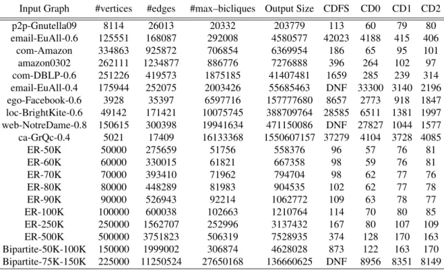
Table 3.2: Various properties of the input graphs used, and runtime (in seconds) of different algorithms to enumerate all maximal bicliques within the graph using 100 reducers. DNF means that the algo-rithm did not finish in 12 hours. The size threshold was set as1 to enumerate all maximal bicliques. Runtime includes overhead of all MapReduce rounds including graph clustering, i.e. formation of 2– neighborhood.
Input Graph #vertices #edges #max–bicliques Output Size CDFS CD0 CD1 CD2 p2p-Gnutella09 8114 26013 20332 203779 113 60 79 80 email-EuAll-0.6 125551 168087 292008 4580577 42023 4188 415 406 com-Amazon 334863 925872 706854 6369954 186 65 95 101 amazon0302 262111 1234877 886776 7276888 396 264 102 97 com-DBLP-0.6 251226 419573 1875185 41407481 1659 285 239 314 email-EuAll-0.4 175944 252075 2003426 55685463 DNF 33300 3140 2196 ego-Facebook-0.6 3928 35397 6597716 157777680 8657 2773 918 1847 loc-BrightKite-0.6 49142 171421 10075745 388709764 28585 6511 1381 1997 web-NotreDame-0.8 150615 300398 19941634 471150086 DNF 27827 1044 1577 ca-GrQc-0.4 5021 17409 16133368 1550607157 37279 4104 3728 4085 ER-50K 50000 275659 51756 558376 96 57 76 81 ER-60K 60000 330015 61821 667358 98 59 76 81 ER-70K 70000 393410 71962 794704 98 62 77 76 ER-80K 80000 448289 81983 904535 102 62 77 78 ER-90K 90000 526943 92214 1062772 109 63 78 77 ER-100K 100000 600038 102663 1210764 114 70 80 85 ER-250K 250000 1562707 252996 3137432 167 80 107 109 ER-500K 500000 3751823 506319 7528935 374 128 170 163 Bipartite-50K-100K 150000 1999002 306874 4628028 873 122 163 170 Bipartite-75K-150K 225000 11250524 27650168 136660625 DNF 8956 8351 8149