June 23, 2003 6:36 00730
International Journal of Bifurcation and Chaos, Vol. 13, No. 6 (2003) 1383–1422 c
World Scientific Publishing Company
RECENT DEVELOPMENTS IN CHAOTIC
TIME SERIES ANALYSIS
YING-CHENG LAI
Department of Mathematics and Statistics, Department of Electrical Engineering, Arizona State University, Tempe, AZ 85287, USA
NONG YE
Department of Industrial Engineering, Department of Computer Science and Engineering,
Arizona State University, Tempe, AZ 85287, USA Received June 6, 2002
In this paper, two issues are addressed: (1) the applicability of the delay-coordinate embedding method totransientchaotic time series analysis, and (2) the Hilbert transform methodology for chaotic signal processing.
A common practice in chaotic time series analysis has been to reconstruct the phase space by utilizing the delay-coordinate embedding technique, and then to compute dynamical invariant quantities of interest such as unstable periodic orbits, the fractal dimension of the underlying chaotic set, and its Lyapunov spectrum. As a large body of literature exists on applying the technique to time series from chaotic attractors, a relatively unexplored issue is its applica-bility to dynamical systems that exhibit transient chaos. Our focus will be on the analysis of transient chaotic time series. We will argue and provide numerical support that the current delay-coordinate embedding techniques for extracting unstable periodic orbits, for estimating the fractal dimension, and for computing the Lyapunov exponents can be readily adapted to transient chaotic time series.
A technique that is gaining an increasing attention is the Hilbert transform method for signal processing in nonlinear systems. The general goal of the Hilbert method is to assess the spectrum of the instantaneous frequency associated with the underlying dynamical process. To obtain physically meaningful results, it is necessary for the signal to possess a proper rotational structure in the complex plane of the analytic signal constructed by the original signal and its Hilbert transform. We will describe a recent decomposition procedure for this task and apply the technique to chaotic signals. We will also provide an example to demonstrate that the methodology can be useful for addressing some fundamental problems in chaotic dynamics.
Keywords: Chaotic time series; delay coordinates; embedding; transient chaos; correlation dimen-sion; Lyapunov exponents; unstable periodic orbits; Hiebert transform; instantaneous frequency.
1. Introduction
Parallel to the rapid development of nonlinear dy-namics since the late seventies, there has been a tremendous amount of effort on data analysis.
Suppose an experiment is conducted and some time series are measured. Such a time series can be, for instance, a voltage signal from a physical or biologi-cal experiment, or the concentration of a substance in a chemical reaction, or the EEG signals from a
patient with epileptic seizures, or the amount of instantaneous traffic at a point in the internet, and so on. The general question is: what can we say about the underlying dynamical system that gen-erates the time series, if the equations governing the time evolution of the system are unknown and the only available information about the system is the measured time series?
This paper reviews two approaches in nonlin-ear data analysis: (1) the delay-coordinate embed-ding technique [Takens, 1981], and (2) the time-frequency method based on the Hilbert transform [Huang et al., 1998]. The embedding method has been proven useful, particularly for time series from low-dimensional, deterministic or mostly determin-istic1 dynamical systems. That is, for situations where the dynamical invariant set responsible for the behavior of the measured time series is low-dimensional and the influence of noise is relatively small, the delay-coordinate embedding method can yield reliable information essential for understand-ing the underlyunderstand-ing dynamical system. The method has been applied to many disciplines of science and engineering [Abarbanel, 1996; Kantz & Schreiber, 1997], and it is also the key to controlling chaos [Ottet al., 1990; Garfinkelet al., 1992; Schiffet al., 1994; Boccalettiet al., 2000], one of the most fruit-ful areas in applicable chaotic dynamics in the last decade [Chen, 1999].
The mathematical foundation of the delay-coordinate embedding technique was laid by Takens in his seminal paper [Takens, 1981]. He proved that, under fairly general conditions, the underlying dy-namical system can be faithfully reconstructed from time series in the sense that, a one-to-one corre-spondence can be established between the recon-structed and the true but unknown dynamical sys-tems. Based on the reconstruction, quantities of importance for understanding the system can be es-timated, such as the relative weights of determinis-ticity and stochasdeterminis-ticity embedded in the time series, the dimensionality of the underlying dynamical sys-tem, the degree of sensitivity on initial conditions as characterized by the Lyapunov exponents, and unstable periodic orbits that constitute the skele-ton of the invariant set responsible for the observed dynamics.
There exists a large body of literature on the application of the delay-coordinate embedding
technique to dynamical systems with chaotic attrac-tors [Abarbanel, 1996; Kantz & Schreiber, 1997]. Time series obtained from such a system can in principle be as long as one wishes. Another common situation of interest is where the dynamical system exhibits only transient chaos [Grebogi et al., 1982, 1983; Grassberger & Kantz, 1985; T´el, 1990, 1996]. For such a system, a measured signal exhibits a ran-dom behavior during an initial time interval before finally settling into a nonchaotic state. The con-ventional wisdom may be simply to disregard the transient portion of the data and to concentrate on the final state. By doing this, however, information about the system may be lost, because the irregu-lar part of the data may contain important hints about the system dynamics. Transient chaos is in fact ubiquitous in dynamical systems. In view of this, analyzing transient chaotic time series is as important as analyzing sustained chaotic data, yet to our knowledge, the problem has begun to be ad-dressed only recently [Janosi & T´el, 1994; Dhamala et al., 2000, 2001].
It has been known that the dynamical invari-ant sets responsible for transient chaos are nonat-tracting chaotic saddles [Grebogiet al., 1982, 1983; Grassberger & Kantz, 1985; T´el, 1990, 1996]. Here, “nonattracting” means that a trajectory starting from a typical initial condition in a phase-space region containing the saddle stays near the sad-dle for a finite amount of time exhibiting chaotic behavior, exits the region, and approaches asymp-totically to a final state. Chaotic saddles are com-mon in nonlinear dynamical systems. For instance, a chaotic saddle can arise after a chaotic attractor is destroyed at crisis [Grebogi et al., 1982, 1983]. Or, a saddle can be found in every periodic win-dow where it coexists with a periodic attractor. Physically, chaotic saddles lead to observable phenomena such as chaotic scattering [T´el & Ott, 1993], fractal basin boundaries [McDonald et al., 1985], fractal concentrations of passive particles advected in open hydrodynamical flows [Jones & Aref, 1988; Jones et al., 1989; Young & Jones, 1991; Jung & Ziemniak, 1992; Jung et al., 1993; Ziemniak et al., 1994; P´entek et al., 1995; Stolovitzky et al., 1995; Karolyi & T´el, 1997], and fractal distribution of chemicals in environmental flows [Toroczkai et al., 1998; K´arolyi et al., 1999; Nishikawa et al., 2002]. Mathematically, chaotic
1
In realistic situations environmental noise is inevitable. Here “mostly deterministic” means that the system evolves according to a set of determinsitic rules, under the influence of small noise.
June 23, 2003 6:36 00730
Recent Developments in Chaotic Time Series Analysis 1385
saddles are closed, bounded, and invariant sets with dense orbits. They are the “soul” of chaotic dynam-ics [Smale, 1967].
One focus of this paper will then be on ana-lyzing time series from transient chaotic systems. The following problems will be addressed: (1) de-tecting unstable periodic orbits, (2) estimating the correlation dimension, and (3) computing the Lyapunov exponents. The main point is that, de-spite the difficulty in dealing with a transient chaotic system for which the chaotic phases con-taining the essential information about the system are short, many of the standard algorithms that are used to estimate dynamical quantities from time se-ries of sustained chaotic processes can be applied to ensembles of transient chaotic time series. It is not necessary to construct a single long time series from a set of shorter ones. All that is required is a collec-tion of transient time series, starting from different initial conditions. Section 2 is devoted to the es-sential features of the delay-coordinate embedding technique and various methods for computing the dynamical invariants from transient chaotic time series.
The Hilbert-transform based time-frequency method [Huanget al., 1998] can be applied to non-linear and/or nonstationary time series. The tech-nique can in principle be applied to random and nonstationary time series, and it can be useful if one is interested in analyzing the system in terms of the distribution of the instantaneous, physical frequen-cies.2 In certain circumstances the time-frequency method can be powerful for identifying the phys-ical mechanisms responsible for the characteristics of the instantaneous-frequency spectrum of the data [Huanget al., 1998].
The time-frequency method to be described in this paper aims to extract the fundamental phys-ical frequencies from chaotic time series. Roughly, a random but bounded time series implies recur-rence in time of the measured physical quantity. The recurrence can be regarded, conceptually, as being composed of rotations in a physical or mathemat-ical space. The questions are: how many principal rotations exist and what are the frequency char-acteristics of these rotations? The recent ground-breaking idea by Huang et al. [1998] leads to a powerful technique that provides answers to these questions. It should be stressed here that the
fre-quency components here correspond to rotations and, hence, they are different from these in the traditional Fourier analysis or in the wavelet anal-ysis. In many situations the instantaneous fre-quencies of the rotations contain much more in-formation than the Fourier or wavelet frequency components that are associated with simple mathe-matical functions such as the harmonics. The in-stantaneous frequencies of rotations can thus be physically more meaningful. While Fourier and wavelet analyses are well developed methods for sig-nal processing in linear systems, Huanget al.argue that the Hilbert analysis is fundamentally superior to both the Fourier and wavelet analyses for non-stationary and nonlinear time series [Huang et al., 1998]. Section 3 will detail concepts such as rota-tions and instantaneous frequencies, analytic sig-nals, and the Hilbert transform, describe the cor-responding decomposition technique developed by Huanget al.[1998], and illustrate that the method-ology can be applied to chaotic systems. For com-pleteness, at the beginning of Sec. 3, we briefly re-view the Fourier spectral and wavelet methods.
2. Embedding Method for Chaotic Time Series Analysis
2.1. Reconstruction of phase space Let ui(t) (i= 1, . . . , l) be a set of l measurements. In principle, the measured time series come from an underlying dynamical system that evolves the state variable in time according to a set of deter-ministic rules, which are generally represented by a set of differential equations, with or without the influence of noise. Mathematically, any such set of differential equations can be easily converted to a set of first-order, autonomous equations. The dy-namical variables from all the first-order equations constitute thephase space, and the number of such variables is thedimensionof the phase space, which we denote by M. The phase-space dimension can in general be quite large. For instance, in a fluid experiment, the governing equation is the Navier– Stokes equation which is a nonlinear partial dif-ferential equation. In order to represent the sys-tem by first-order ordinary differential equations via, say, the procedure of spatial discretization, the number of required equations is infinite. The phase-space-dimension in this case is thus infinite.
2
However, it often occurs that the asymptotic evo-lution of the system lives on a dynamical invariant set of only finite dimension. The assumption here is that the details of the system equations in the phase space and of the asymptotic invariant set that deter-mines what can be observed through experimental probes, are unknown. The task is to estimate,based solely on one or few time series, practically use-ful statistical quantities characterizing the invariant set, such as its dimension, its dynamical skeleton, and its degree of sensitivity on initial conditions. The delay-coordinate embedding technique estab-lished by Takens [1981] provides a practical solu-tion to this task [Packardet al., 1980]. In particular, Takens’ embedding theorem guarantees that a topo-logical equivalence of the phase space of the intrinsic unknown dynamical system can be reconstructed from time series, based on which characteristics of the dynamical invariant set can be estimated.
Takens’ delay-coordinate embedding method goes, as follows. From each measured time series
ui(t) (i= 1, . . . , l), the following vector quantity of
q components is constructed,
ui(t) ={ui(t), ui(t+τ), . . . , ui[t+ (q−1)τ]}, where τ is the delay time. Since there are l time series, a vector with m ≡ ql components can be constructed, as follows:
x(t) ={u1(t), u2(t), . . . ,ul(t)}
={u1(t), u1(t+τ), . . . , u1[t+ (q−1)τ],
u2(t), u2(t+τ), . . . , u2[t+ (q−1)τ], . . . ,
ul(t), ul(t+τ), . . . , ul[t+ (q−1)τ]}, (1) where m is the embedding dimension. Clearly, the delay time τ and the embedding dimension m
are the two fundamental parameters in the delay-coordinate embedding method.
1.Delay time τ. In order for the time-delayed com-ponents ui(t+jτ) (j = 1, . . . , q−1) to serve as independent variables, the delay timeτ needs to be chosen carefully. Roughly, if τ is too small, then adjacent components ui(t) and ui(t + τ) will be too correlated for them to serve as independent coordinates. If, on the other hand, τ is too large, then neighboring components are too uncorrelated for the purpose. Empirically, one can examine the autocorrelation function of ui(t) and decide a proper delay time [Theiler, 1986]. In particular, one
computes
c(T)≡ hui(t)ui(t+T)i
hu2i(t)i ,
where h·i stands for time average. The delay time
τ can be chosen to be the value of T such that
c(T)/c(0)≈e−1.
There exist various alternative empirical meth-ods for choosing a proper delay time [Liebert & Schuster, 1989; Liebert et al., 1991; Buzug & Pfister, 1992; Kember & Fowler, 1993; Rosenstein et al., 1994], which all yield similar results. A firmer theoretical foundation may be possible by explor-ing the statistics for testexplor-ing continuity and differ-entiability from chaotic time series proposed by Pecoraet al.[Pecora et al., 1995; Pecora & Carroll, 1996; Pecora et al., 1997; Pecora & Carroll, 2000; Goodridgeet al., 2001].
2.Embedding dimensionm. In order to have a faith-ful representation of the true dynamical system, the embedding dimensionmshould be sufficiently large. Takens’ theorem [Takens, 1981] provides a lower bound for m. In particular, suppose the dynami-cal invariant set lies in a d-dimensional manifold (or subspace) in the phase space. Then, ifm >2d, them-dimensional reconstructed vectors x(t) have a one-to-one correspondence to the vectors of the true dynamical system. This result can be under-stood by the following simple mathematical argu-ment. Consider two smooth surfaces of dimensions
d1 and d2 in an M-dimensional space and
exam-ine the set of their intersections. The question is whether they intersect generically in the sense that the intersections cannot be removed by small per-turbations to either surface. The natural approach is then to look at the dimensiondI of the intersect-ing set, which is
dI =d1+d2−M .
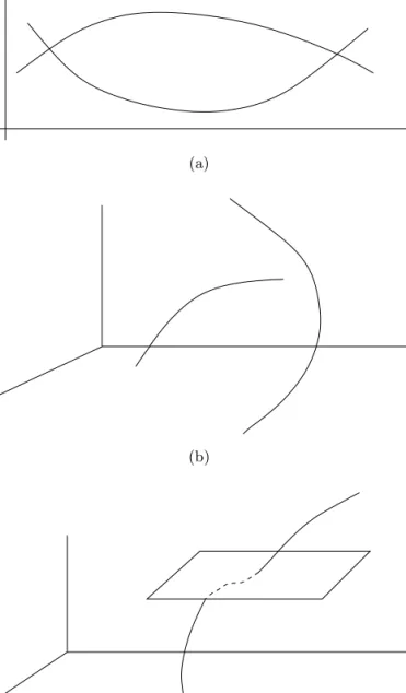
If dI ≥ 0, the intersection is generic. For exam-ple, consider the intersection of two one-dimensional curves in a two-dimensional plane:d1 =d2= 1 and
M = 2. We obtain: dI = 0, which means that the intersecting set consists of points, and the intersec-tions are generic because small perturbaintersec-tions can-not remove them. If, however, M = 3, then dI < 0, which means that two one-dimensional curves do not intersect generically in a three-dimensional space. These two cases, together with an additional one (d1 = 1, d2 = 2, and M = 3), are illustrated
June 23, 2003 6:36 00730
Recent Developments in Chaotic Time Series Analysis 1387
(c)
(b)
(a)
(a)(c)
(b)
(a)
(b)(c)
(b)
(a)
(c)Fig. 1. Illustration of generic and nongeneric intersections of simple geometric sets: (a)d1=d2= 1 andM = 2 (generic
intersection), (b) d1 = d2 = 1 andM = 3 (nongeneric
in-tersection), and (c) d1 = 1, d2 = 2, and M = 3 (generic
intersection).
whether the dynamical invariant set would inter-sect itself in the reconstructed phase space. In or-der to obtain a one-to-one correspondence between points on the invariant sets in the actual and re-constructed phase spaces, self-intersection must not occur. Thus, taking d1 = d2 = d and M = m, no
self-intersection requiresdI <0, which means that
m >2d.
While Takens’ theorem assumes that the rele-vant dimensiondof the set is that of the manifold in which the set lies, this dimension can be quite dif-ferent from the dimension of the set itself, which is
physically more relevant. The work by Sauer, Yorke, and Casdagli [Sauer et al., 1991] extends Takens’s theorem to relax the dimension requirement: the dimension d can in fact be the box-counting di-mension D0 [Farmer et al., 1983] of the invariant
set.
2.2. Detection of unstable periodic orbits
A fundamental feature that differs a deterministic chaotic system from a stochastic one is the exis-tence of an infinite number of unstable periodic orbits which constitute the skeleton of the chaotic invariant set [Auerbach et al., 1987; Gunaratne & Procaccia, 1987; Moritaet al., 1987; Grebogiet al., 1988; Biham & Wenzel, 1989; Lai et al., 1997; Lai, 1997; Zoldi & Greenside, 1998; Davidchack et al., 2000]. Computation of unstable periodic or-bits from system equations [Biham & Wenzel, 1989; Schmelcher & Diakonos, 1997, 1998; Schmelcher et al., 1998; Davidchack & Lai, 1999; Davidchack et al., 2001; Pingel et al., 2001] and their detec-tion from experimental time series have been an ac-tive area of research [Lathrop & Kostelich, 1989; Mindlin et al., 1990; Pawelzik & Schuster, 1991; Badii et al., 1994; Pierson & Moss, 1995; Christini & Collins, 1995; Pei & Moss, 1996a, 1996b; Soet al., 1996, 1997; Allie & Mees, 1997; Dhamala et al., 2000, 2001]. At a fundamental level, unstable pe-riodic orbits embedded in a chaotic invariant set are related to its natural measure [Grebogi et al., 1988; Laiet al., 1997; Lai, 1997], which is the base for defining physically important quantities such as the fractal dimensions and Lyapunov exponents. At a practical level, successful detection of unstable pe-riodic orbits indicates the deterministic origin of the underlying dynamical process. In what follows, we will review the basic concepts of the natural mea-sure and unstable periodic orbits, describe an algo-rithm for their detection from chaotic time series, and provide numerical examples.
2.2.1. The natural measure: why are
unstable periodic orbits important?
One of the most important problems in dealing with a chaotic system is to compute long term statistics such as averages of physical quantities, Lyapunov exponents, dimensions, and other invariants of the probability density or the measure. The interest in
the statistics roots in the fact that trajectories of de-terministic chaotic systems are apparently random and ergodic. These statistical quantities, however, are physically meaningful only when the measure being considered is the one generated by a typi-cal trajectory in the phase space. This measure is called the natural measure and it is invariant under the evolution of the dynamics [Grebogiet al., 1988]. The importance of the natural measure can be assessed by examining how trajectories behave in a chaotic system. Due to ergodicity, trajectories on a chaotic set exhibit sensitive dependence on ini-tial conditions. Moreover, the long-time probabil-ity distribution generated by a typical trajectory on the chaotic set is generally highly singular.3 For a chaotic attractor, a trajectory originated from a random initial condition in the basin of attraction visits different parts of the attractor with drasti-cally different probabilities. Call regions with high probabilities “hot” spots and regions with low prob-abilities “cold” spots. Such hot and cold spots in the attractor can in general be interwoven on arbitrarily fine scales. In this sense, chaotic attractors are said to possess a multifractal structure. Due to this sin-gular behavior, one utilizes the concept of the natu-ral measure to characterize chaotic attractors [Ott, 1993]. To obtain the natural measure, one covers the chaotic attractor with a grid of cells and exam-ine the frequencies with which a typical trajectory visits these cells in the limit that both the length of the trajectory goes to infinity and the size of the grid goes to zero [Farmeret al., 1983]. Except for an initial condition set of Lebesgue measure zero in the basin of attraction, these frequencies in the cells are the natural measure. Specifically, letf(x0, T, εi) be the amount of time that a trajectory from a random initial conditionx0in the basin of attraction spends
in theith covering cellCi of edge lengthεiin a time
T. The probability measure of the attractor in the cell Ci is µi = lim εi→0 lim T→∞ f(x0, T, εi) T . (2)
The measure is called natural if it is the same for all randomly chosen initial conditions, that is, for all initial conditions in the basin of attraction ex-cept for a set of Lebesgue measure zero. The spec-trum of an infinite number of fractal dimensions
quantifies the behavior of the natural measure for multifractal chaotic attractors [Grassberger & Procaccia, 1983a].
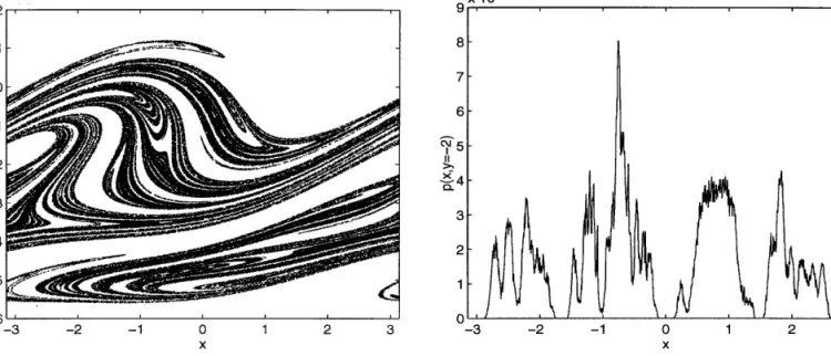
The above description can be seen by con-sidering a physical example, the forced damped pendulum dx dt =y , dy dt =−0.05y−sin x+ 2.5 sint . (3)
Figure 2(a) plots [Lai, 1997], on the stroboscopic surface of section defined at discrete times tn = 2πn, n= 1, . . . ,a trajectory of 1.5×10⁵ points on
the chaotic attractor, where the abscissa and the ordinate are the anglex(tn) and the angular veloc-ity y(tn) ≡dx/dt|tn of the pendulum, respectively.
Figure 2(b) shows the one-dimensional probability distribution on the attractor at y=−2. To obtain Fig. 2(b), a one-dimensional array of 1000 rectangu-lar cells is defined in thex-direction aty=−2. The frequency of visits to each cell is then computed by utilizing a trajectory of 107 points on the surface of section. In fact, probability distributions on any line intersecting the chaotic attractor exhibit simi-lar behavior. These results suggest a highly singusimi-lar probability distribution on the chaotic attractor.
Because of the physical importance of the nat-ural measure, it is desirable be able to understand and characterize it in terms of the fundamental dy-namical quantities of the chaotic set. There is noth-ing more fundamental than to express the natural measure in terms of the periodic orbits embedded in a chaotic attractor.
A chaotic set has embedded within itself an infinite number of unstable periodic orbits. These periodic orbits are atypical in the sense that they form a Lebesgue measure zero set. With probability one, randomly chosen initial conditions do not yield trajectories which live on unstable periodic orbits. Invariant measures produced by unstable periodic orbits are thus atypical, and there is an infinite number of such atypical invariant measures embed-ded in a chaotic attractor. The “hot” and “cold” spots are a reflection of these atypical measures. The natural measure, on the other hand, is typical in the sense that it is generated by a trajectory orig-inated from any one of the randomly chosen initial
3
Take, for example, the logistic mapxn+1= 3.8xn(1−xn) that exhibits a chaotic attractor. A simple argument [Ott, 1993] based on mapping of the probability in a small interval suggests that singularities in the probability distribution occurs at all forward images of the critical pointxc= 1/2 under the map, which are dense in the attractor.
June 23, 2003 6:36 00730
Recent Developments in Chaotic Time Series Analysis 1389
(a) (b)
Fig. 2. For the forced damped pendulum system Eq. (3), (a) a trajectory of 1.5×10⁵points on the chaotic attractor on the stroboscopic surface of section, and (b) the distribution of the natural measure in a one-dimensional array of 1000 rectangular cells in thex-direction at y = 2. The size of each cell is 2π/1000×0.06. Numerically, the total measure contained in the attractor is normalized to unity. Apparently, the natural measure is singular.
conditions in the basin of attraction. A typical tra-jectory visits a fixed neighborhood of any one of the periodic orbits from time to time. Thus, chaos can be considered as being organized with respect to the unstable periodic orbits [Auerbachet al., 1987; Gunaratne & Procaccia, 1987].
Grebogi, Ott, and Yorke derived [Grebogiet al., 1988], for the special case of hyperbolic chaotic sys-tems,4 a formula relating the natural measure of the chaotic set in the phase space to the expand-ing eigenvalues of all the periodic orbits embedded in the set. Specifically, consider an N-dimensional mapM(x). Let xip be the ith fixed point of thep -times iterated map, i.e. Mp(xip) =xip. Thus each
xip is on a periodic orbit whose period is either p or a factor of p. The natural measure of a chaotic attractor in a phase-space region S is given by
µ(S) = lim p→∞ X xip∈S 1 L1(xip, p) , (4) where L1(xip, p) is the magnitude of the expand-ing eigenvalue of the Jacobian matrix DMp(xip),
and the summation is taken over all fixed points of Mp(x) in S. This formula can be derived under the assumption that the phase space can be divided into cells via a Markov partition, a condition that is generally satisfied by hyperbolic chaotic systems. Explicit verification of this formula was done for several analyzable hyperbolic maps [Grebogiet al., 1988]. Equation (4) is theoretically significant and interesting because it provides a fundamental link between the natural measure and various atypical invariant measures embedded in a chaotic attrac-tor. The applicability of Eq. (4) to nonhyperbolic chaotic systems has also been addressed recently [Lai et al., 1997; Lai, 1997].
2.2.2. Extracting unstable periodic orbits
from transient chaotic time series
A powerful algorithm for detecting unstable pe-riodic orbits from chaotic time series is due to Lathrop and Kostelich (LK) [Lathrop & Kostelich, 1989]. The method is based on identifying sets of
4
The dynamics is hyperbolic on a chaotic set if at each point of the trajectory the phase space can be split into an expanding and a contracting subspaces and the angle between them is bounded away from zero. Furthermore, the expanding subspace evolves into the expanding one along the trajectory and the same is true for the contracting subspace. Otherwise the set is nonhyperbolic. In general, nonhyperbolicity is a complicating feature because it can cause fundamental difficulties in the study of the chaotic systems, such as the shadowability of numerical trajectories by true trajectories [Hammelet al., 1987, 1988; Grebogiet al., 1990; Dawsonet al., 1994; Laiet al., 1999a; Lai & Grebogi, 1999; Laiet al., 1999b].
recurrent points in the reconstructed phase space. To do this, one first reconstructs a phase-space trajectory x(t) from a measured scalar time se-ries{u(t)}by using the delay-coordinate embedding method described in Sec. 2.1. To identify unstable periodic orbits, one follows the images of x(t) un-der the dynamics until a value t1 > t is found such
that kx(t1)−x(t)k < ε, where ε is a prespecified
small number that defines the size of the recurrent neighborhood atx(t). In this case, x(t) is called an (T, ε) recurrent point, and T = t1 −t is the
re-currence time. A recurrent point is not necessarily a component of a periodic orbit of period T. How-ever, if a particular recurrence time T appears fre-quently in the reconstructed phase space, it is likely that the corresponding recurrent points are close to periodic orbits of period T. The idea is then to construct a histogram of the recurrence times and identify peaks in the histogram. Points that occur frequently are taken to be, approximately, compo-nents of the periodic orbits. The LK-algorithm has been used to detect unstable periodic orbits, for in-stance, from measurements of a chaotic chemical reaction [Lathrop & Kostelich, 1989].
More recently, the LK algorithm has been adapted to detecting unstable periodic orbits from short, transiently chaotic series [Dhamala et al., 2000]. The reason that the LK-algorithm is appli-cable to transient time series lies in the statisti-cal nature of this method, as a histogram of re-currence times can be obtained even with short time series. Provided that there is a large num-ber of such time series so that a good statistics of the recurrence times can be obtained, unstable periodic orbits embedded in the underlying chaotic set can be identified. It is not necessary to concate-nate many short time series to form a single long one (such concatenations are invariably problematic [Janosi & T´el, 1994]). Intuitively, since the time se-ries are short, periodic orbits of short periods can be detected.
To demonstrate the LK-algorithm, here we take the numerical examples reported in [Dhamalaet al., 2000] with the following chaotic R¨ossler system [R¨ossler, 1976]: dx dt =−y−z , dy dt =x+ay , (5) dz dt =b+ (x−c)z ,
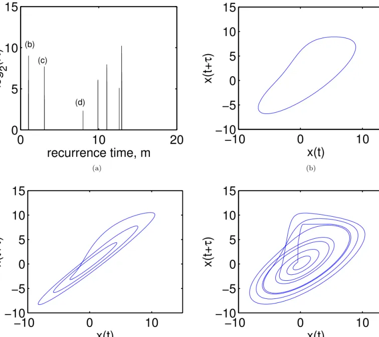
where a, b, and c are parameters. There is tran-sient chaos when the set of parameter values yields a periodic window in which a stable periodic at-tractor and a chaotic saddle coexist. For instance, for a =b = 0.2 and c = 5.3, the system falls in a periodic window of period 3. Typical measurement of a dynamical variable, say x(t), exhibits chaotic behavior for a finite amount of time before settling in the period-3 attractor. In [Dhamalaet al., 2000], 10 such time series are generated by integrating the R¨ossler system from different initial conditions, and the corresponding time seriesx(t) for 0≤t≤4 are recorded. The lifetime of the chaotic transient is about 4. These time series are assumed to be the only available information about the system. For each time series, a seven-dimensional vector space is reconstructed by using the delay time τ = 0.02. To obtain recurrence times, it is necessary to deter-mineε, the size of the recurrent neighborhood. The value ofεmust not be large to avoid too many false positives, butε must not be so small that genuine recurrences are missed. Typically, it is found in nu-merical experiments that the number of recurrences
N(ε) increases with the length and the number of the individual transient trajectories, and withε. It tends to saturate whenε is too large. The value of
εat which N(ε) saturates is taken to be an appro-priate size of the recurrent neighborhood. For the R¨ossler system, ε = 2% of the root-mean-square (rms) value of the chaotic signal is used [Dhamala et al., 2000]. Figure 3(a) shows the histogram of the recurrence times for the 10 transient chaotic time series from the period-3 window. Figures 3(b)– 3(d) show, in the plane of x(t) versus x(t + τ), three recurrent orbits. The orbit in Fig. 3(b) has the shortest recurrence time, so it is a “period-1” orbit. Figures 3(c) and 3(d) show a period-3 and a period-8 orbits, respectively. The orbits are selected from the set of recurrent points comprising the cor-responding peak in the histogram. In general, it is found [Dhamalaet al., 2000] that the LK-algorithm is capable of yielding many periodic orbits of low periods.
In an experimental setting, time series are contaminated by dynamical and/or observational noise. A question is whether periodic orbits can still be extracted from noisy transient chaotic time series. Qualitatively, under the influence of noise, the effective volume of recurrent region in the
June 23, 2003 6:36 00730
Recent Developments in Chaotic Time Series Analysis 1391
0
10
20
0
5
10
15
recurrence time, m
log
2
(N)
−10
0
10
−10
−5
0
5
10
15
x(t)
x(t+
τ
)
−10
0
10
−10
−5
0
5
10
15
x(t)
x(t+
τ
)
−10
0
10
−10
−5
0
5
10
15
x(t)
x(t+
τ
)
(b) (c) (d)0
10
20
0
5
10
15
recurrence time, m
log
2
(N)
−10
0
10
−10
−5
0
5
10
15
x(t)
x(t+
τ
)
−10
0
10
−10
−5
0
5
10
15
x(t)
x(t+
τ
)
−10
0
10
−10
−5
0
5
10
15
x(t)
x(t+
τ
)
(b) (c) (d) (a) (b)0
10
20
0
5
10
15
recurrence time, m
log
2
(N)
−10
0
10
−10
−5
0
5
10
15
x(t)
x(t+
τ
)
−10
0
10
−10
−5
0
5
10
15
x(t)
x(t+
τ
)
−10
0
10
−10
−5
0
5
10
15
x(t)
x(t+
τ
)
(b) (c) (d)0
10
20
0
5
10
15
recurrence time, m
log
2
(N)
−10
0
10
−10
−5
0
5
10
15
x(t)
x(t+
τ
)
−10
0
10
−10
−5
0
5
10
15
x(t)
x(t+
τ
)
−10
0
10
−10
−5
0
5
10
15
x(t)
x(t+
τ
)
(b) (c) (d) (c) (d)Fig. 3. For the R¨ossler system: (a) histogram of the recurrence timeT, (b–d) a period-1, a period-3, and a period-8 recurrent orbits extracted from the histogram in (a), respectively.
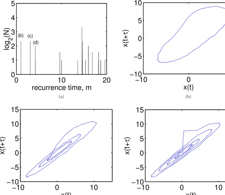
phase space decreases and, hence, a decrease in the number of recurrences is expected. Figures 4(a)– 4(d) show the number of recurrent points (a) and three periodic orbits extracted from 10 transient chaotic time series with additive noise of the form
G(0, 0.01), a normal (Gaussian) distribution cen-tered at 0 with variance 0.01. This noise level rep-resents a rms value that is approximately 0.5% of that of the chaotic signal. It can be seen that at this low noise level, periodic orbits can still be reliably detected. It is found, however, that for the R¨ossler system at ε = 2% of the rms value of the chaotic signal with noise beyond 1%, no periodic orbits can
be extracted from the histogram of recurrences. One way to assess the influence of noise is to compute, at several fixed values of ε, how the number of recur-rent points decreases as the noise amplitude (η) is increased. Figures 5(a) and 5(b) show the result of such computations for (a)ε= 2% and (b)ε= 6% of the rms value of the signal. It can be seen that the number of recurrent points goes to zero atη≈ε/2, which can be understood, as follows. Under noise of amplitude η, both the center and the boundary of the recurrent region are uncertain within η. Thus, the effective phase-space volume in d dimensions in which two points can still be considered within
0
10
20
0
1
2
3
4
5
recurrence time, m
log
2
(N)
−10
0
10
−10
−5
0
5
10
x(t)
x(t+
τ
)
−10
0
10
−10
−5
0
5
10
15
x(t)
x(t+
τ
)
−10
0
10
−10
−5
0
5
10
15
x(t)
x(t+
τ
)
(b) (c) (d)0
10
20
0
1
2
3
4
5
recurrence time, m
log
2
(N)
−10
0
10
−10
−5
0
5
10
x(t)
x(t+
τ
)
−10
0
10
−10
−5
0
5
10
15
x(t)
x(t+
τ
)
−10
0
10
−10
−5
0
5
10
15
x(t)
x(t+
τ
)
(b) (c) (d) (a) (b)0
10
20
0
1
2
3
4
5
recurrence time, m
log
2
(N)
−10
0
10
−10
−5
0
5
10
x(t)
x(t+
τ
)
−10
0
10
−10
−5
0
5
10
15
x(t)
x(t+
τ
)
−10
0
10
−10
−5
0
5
10
15
x(t)
x(t+
τ
)
(b) (c) (d)0
10
20
0
1
2
3
4
5
recurrence time, m
log
2
(N)
−10
0
10
−10
−5
0
5
10
x(t)
x(t+
τ
)
−10
0
10
−10
−5
0
5
10
15
x(t)
x(t+
τ
)
−10
0
10
−10
−5
0
5
10
15
x(t)
x(t+
τ
)
(b) (c) (d) (c) (d)Fig. 4. For a noisy R¨ossler system: (a) histogram of the recurrence time T, (b–d) a period-1, a period-2, and a period-4 recurrent orbits extracted from the histogram in (a), respectively, whereε= 6% and the rms value of the noise is at about 0.5% of that of the chaotic signal.
distanceε(recurrent) is proportional to (ε−η)d−ηd, which vanishes atη =ε/2. Sinceεshould be small to guarantee recurrence, we see that the tolerable noise level is also small.
2.2.3. Detectability of unstable periodic
orbits from transient chaotic time series
An issue of interest concerns the detectability of unstable periodic orbits from chaotic time series [Pei et al., 1998]. This is particularly relevant for
transient chaos because trajectories on a chaotic saddle have an average lifetime timeτ staying near the saddle and, hence, it is difficult for a typical tra-jectory to contain periodic orbits of period larger than τ. Effort may then be devoted to connect short time series so that the resulting long time se-ries would contain periodic orbits of larger period [Janosi & T´el, 1994]. Such a task may be difficult. If one fails to detect periodic orbits of high peri-ods, the question is whether one should attempt to increase the number of measurements so that more time series are available. Or, one may attempt
June 23, 2003 6:36 00730
Recent Developments in Chaotic Time Series Analysis 1393
0 0.5 1 1.5 2 2.5 3 3.5 0 0.5 1 noise % N/N 0 ε = 2% 0 0.5 1 1.5 2 2.5 3 3.5 0 0.5 1 noise % N/N 0 ε = 6% (a) 0 0.5 1 1.5 2 2.5 3 3.5 0 0.5 1 noise % N/N 0 ε = 2% 0 0.5 1 1.5 2 2.5 3 3.5 0 0.5 1 noise % N/N 0 ε = 6% (b)
Fig. 5. For the noisy R¨ossler system, the relative number (N/N0) of recurrent points versus the amplitude of noise for two
values of the size of the recurrent neighborhood: (a)ε= 2% and (b)ε= 6% of the rms value of the signal, whereN0 is the
number of recurrent points at zero amplitude of noise. The vertical line in (b) denotes the noise level at which periodic orbits in Fig. 4 are extracted.
to improve techniques to link these time series, a computationally demanding task because it is es-sentially a problem of optimizing many time series and the computation required in any optimization problem typically increases greatly as the number of elements involved is increased. The main point is that in detecting unstable periodic orbits from transient chaos, the probability of detecting orbits of higher periods is typically exponentially small [Dhamalaet al., 2000, 2001]. This is anintrinsic dy-namical property of the underlying chaotic saddle and, hence, increasing the number of measurements or improving techniques of detection will not help enhance the chance to detect these orbits.
Let Φ(p) be the probability to detect any period-p orbit. A scaling relation for Φ(p) can be derived [Dhamala et al., 2000, 2001] by noting that Φ(p) is actually the probability for a trajec-tory to stay in a small neighborhood of any pe-riodic orbit of period p. For a trajectory to stay
in an ν-neighborhood of all p points of the ith or-bit of period p, the trajectory must come within
δ = νe−λi(p)p of any of the p points when it first
encounters with the periodic orbit, whereλi(p)>0 is the Lyapunov exponent of this orbit. The proba-bility for this event is φi(p) ∼δDi, where Di is the pointwise dimension of any one of the p points of this periodic orbit. The exponential factor e−λi(p)p
is proportional to the natural measure associated with this periodic orbit [Grebogi, et al., 1988]. The probability Φ(p) is the accumulative probability of all φi(p), Φ(p) = K(p) X i=1 φi(p)∼ K(p) X i=1 νDiexp [−λ i(p)Dip], (6) where K(p) is the total number of periodic points of period p. Since λi(p) and Di are the local posi-tive Lyapunov exponent and pointwise dimension of periodic orbits of period p, for large p, we
expect them to obey distributions centered at λ1
and D1, respectively, where λ1 and D1 are the
positive Lyapunov exponent and the information dimension of the chaotic saddle. Thus, the main de-pendence of Φ(p) on p is
Φ(p)∼e−λ1D1p
K(p)∼e(−λ1D1+hT)p =e−γp, (7)
whereγ is the exponential scaling exponent andhT is the topological entropy. The Kaplan–Yorke for-mula can be used for chaotic saddles [Hsu et al., 1988; Huntet al., 1996] to expressD1in terms of the
Lyapunov exponentsλ2<0< λ1and the lifetimeτ,
D1= (λ1−1/τ)(1/λ1 + 1/|λ2|),
which yields the following scaling exponent:
γ =λ1−hT + λ2 1 |λ2| − 1 τ 1 + λ1 |λ2| . (8) Equations (7) and (8) are applicable to chaotic saddles in two-dimensional invertible maps or in three-dimensional flows. Note that for chaotic at-tractors (τ → ∞), we have for the scaling exponent:
γ ≈λ1−hT +λ21/|λ2|.
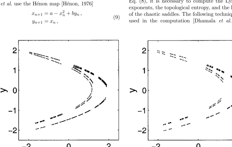
To test Eqs. (7) and (8) numerically, Dhamala et al. use the H´enon map [H´enon, 1976]
xn+1=a−x2n+byn,
yn+1=xn,
(9)
whereaand bare parameters, as unstable periodic orbits in the chaotic saddles of the map can be com-puted systematically [Biham & Wenzel, 1989]. For the following set of three parameter values:a= 1.6, 1.8, and 2.0, there is transient chaos [Lai et al., 1993]. Representative chaotic saddles for a = 1.6 and a = 1.8 are shown in Figs. 6(a) and 6(b), re-spectively, which are obtained by the procedure in [Nusse & Yorke, 1989]. For each value ofa, 106
ini-tial conditions are chosen in the region [−2, 2]× [−2, 2] containing the chaotic saddle, which yield 106 transient time series [Dhamalaet al., 2000]. For
a given period p, the fractions of times that these 106 time series get close to every periodic orbit of
periodpcan be computed. These fractions are used to yield an estimated value for the probability Φ(p), which increases with the number of transient time series and also with the length of the individual tra-jectories. Figures 7(a)–7(d) show ln Φ(p) versus p
for a= 1.6, 1.8, and 2.0, respectively. These plots indicate behavior of exponential decay, and the de-cay exponents are given by the slopes of the plots. To compute the theoretical scaling exponents in Eq. (8), it is necessary to compute the Lyapunov exponents, the topological entropy, and the lifetime of the chaotic saddles. The following techniques are used in the computation [Dhamala et al., 2000,
(a)a= 1.6 (b)a= 1.8
June 23, 2003 6:36 00730
Recent Developments in Chaotic Time Series Analysis 1395
0
10
20
−10
−8
−6
−4
p
ln
Φ
(p)
a = 1.6
0
10
20
−15
−10
−5
p
ln
Φ
(p)
a = 1.8
0
10
20
−15
−10
−5
p
ln
Φ
(p)
a = 2.0
0
10
20
−10
−8
−6
−4
p
ln
Φ
(p)
(a)
a = 1.6
0
10
20
−15
−10
−5
p
ln
Φ
(p)
(b)
a = 1.8
0
10
20
−15
−10
−5
p
ln
Φ
(p)
(c)
a = 2.0
(a) (b)0
10
20
−10
−8
−6
−4
p
ln
Φ
(p)
(a)
a = 1.6
0
10
20
−15
−10
−5
p
ln
Φ
(p)
(b)
a = 1.8
0
10
20
−15
−10
−5
p
ln
Φ
(p)
(c)
a = 2.0
(c)Fig. 7. (a–c) For the H´enon map at a = 1.6, 1.8, and 2.0, ln Φ(p) versus p. The dotted lines indicate the theoretically predicted slopes of ln Φ(p) versusp.
2001]: (1) the procedure to obtain a long trajec-tory on the chaotic saddle [Nusse & Yorke, 1989; Jacobset al., 1997] from which the Lyapunov expo-nents can be computed; (2) the method by Chen et al. [1991] to compute the topological entropy; and (3) the sprinkler method to compute τ [Hsu et al., 1988]. The slopes of the dashed straight lines in Figs. 7(a)–7(d) are the theoretical slopes for the corresponding chaotic saddles. The numerical slopes appear to agree reasonably well with the theoretical ones, as shown further in Table 1, where the numer-ical and theoretnumer-ical slopes, together with the values of other quantities involved in Eq. (8), are listed.
2.3. Computation of dimension
2.3.1. Basics
An often computed dimension in nonlinear time se-ries analysis is the correlation dimension D2, which
is a good approximation of the box-counting di-mension D0: D2 ≤ D0. Grassberger and Procaccia
show in their seminal contribution [Grassberger & Procaccia, 1983b] thatD2can be evaluated by using
the correlation integral C(ε), which is the probabil-ity that a pair of points, chosen randomly in the re-constructed phase space, is separated by a distance less than ε. Let N be the number of points in the
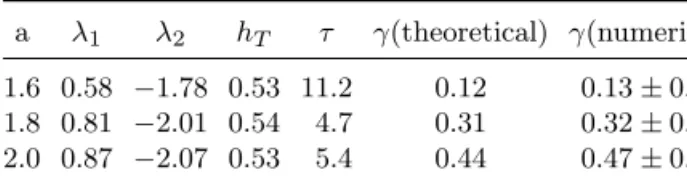
Table 1. Theoretical and numerical values of the scal-ing exponentγat four different parameters for the H´enon map.
a λ1 λ2 hT τ γ(theoretical) γ(numerical) 1.6 0.58 −1.78 0.53 11.2 0.12 0.13±0.04 1.8 0.81 −2.01 0.54 4.7 0.31 0.32±0.03 2.0 0.87 −2.07 0.53 5.4 0.44 0.47±0.04
reconstructed vector time series x(t). The correla-tion integral can be approximated by the following sum, CN(ε) = 2 N(N −1) N X j=1 N X i=j+1 Θ(ε−|xi−xj|), (10) where Θ(·) is the Heaviside function: Θ(x) = 1 for
x ≥ 0 and 0 otherwise, and |xi −xj| stands for the distance between pointsxi andxj. Grassberger and Procaccia argue that the correlation dimension is given by [Grassberger & Procaccia, 1983b]
D2 = lim
ε→0 N→∞lim
log CN(ε)
log ε . (11)
In practice, for a time series of finite length, the sum in Eq. (10) also depends on the embedding dimensionm. Due to such dependencies, the corre-lation dimension D2 is usually estimated by
exam-ining the slope of the linear portion of the plot of log CN(ε) versus log εfor a series of increasing val-ues of m. Form < D2, the dimension of the
recon-structed phase space is not high enough to resolve the structure of the dynamical state and, hence, the slope approximates the embedding dimension. Asm
increases, the resolution of the dynamical state in the reconstructed phase space is improved. Typi-cally, the slope in the plot of logCN(ε) versus log ε increases withmuntil it reaches a plateau; its value at the plateau is then taken as the estimate of
D2 [Grassberger & Procaccia, 1983b; Ding et al.,
1993]. For an infinite and noiseless time series, the value ofmat which this plateau begins to satisfy is
m = Ceil(D2), where Ceil(D2) is the smallest
inte-ger greater than or equal to D2 [Dinget al., 1993].
In a realistic situation, short data sets and observa-tional noise can cause the plateau onset to occur at a value ofmwhich can be larger than Ceil(D2). Even
so, the embedding dimension at which the plateau is reached still provides a reasonably sharp upper bound for the true correlation dimension D2.
De-pendencies of the length of the linear scaling re-gion on fundamental parameters such asm, τ, and
mτhave been analyzed systematically in [Laiet al., 1996; Lai & Lerner, 1998].
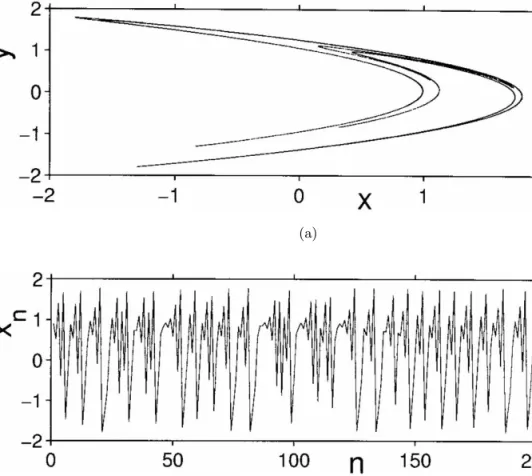
These points can be seen by utilizing the H´enon map Eq. (9) at the standard parameter valuesa= 1.4 and b = 0.3. The map is believed to possess a chaotic attractor, as shown in Fig. 8(a) in the two-dimensional phase space (x, y). A typical time series
{xn}is shown in Fig. 8(b). The theoretical value of the correlation dimension of the chaotic attractor is
D2 ≈1.2 [Laiet al., 1996; Lai & Lerner, 1998].
The GP-algorithm can be applied to estimating the correlation dimension from the time series{xn}. To select the delay timeτ, note that any discrete-time map can be regarded as arising from a Poincar´e surface of section of a continuous-time flow [Ott, 1993]. Thus, one iteration of the map corresponds to roughly one period of oscillation of the continuous-time signal x(t), which, for chaotic systems, is ap-proximately the decay time of the autocorrelation of x(t). As an empirical rule, the delay time can be chosen to be τ = 1 for chaotic time series from discrete-time maps. Equivalently, for chaotic signal
x(t) from a continuous-time flow, the delay time should be chosen approximately as the average pe-riod of oscillation.
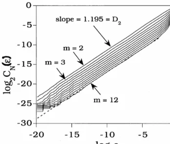
After the delay time τ is chosen, the next step is to compute the correlation integral CN(ε) for a set of systematically increasing values of the embed-ding dimensionm. Figure 9 shows, forN = 2×10⁴, the plots of CN(ε) versus ε on the base-2 logarith-mic scale for m = 1, . . . ,8. The lines are approx-imately linear, and they are parallel for m ≥ 2. Least-squares fits give D2 ≈ 1.2 for m ≥ 2,
indi-cating that the correlation dimension can be esti-mated reliably from a time series by utilizing the GP-algorithm. The saturation of the slope occurs at m = 2, which is the smallest integer above the value of D2. Recall that the embedding
the-orem requires a minimum embedding dimension of 2D0 + 1, which is 4 for the H´enon chaotic
at-tractor. This is because the task here is to es-timate the dimension only, while the embedding theorem guarantees a one-to-one correspondence between the reconstructed and the true chaotic attractors. A dimension estimate does not neces-sarily require such a one-to-one correspondence. For instance, consider a two-dimensional surface in a three-dimensional space. The projection of this surface onto a dimensional plane is still a two-dimensional region. Thus, its dimension can be es-timated even in a two-dimensional subspace.
June 23, 2003 6:36 00730
Recent Developments in Chaotic Time Series Analysis 1397
(a)
(b)
Fig. 8. (a) The H´enon chaotic attractor and (b) a typical chaotic time series.
2.3.2. Applicability of GP algorithm to
transient chaotic time series
An important question is whether the GP paradigm [Eqs. (10) and (11)] is applicable to transient time series from chaotic saddles. Recently, an argument is provided which appears to give an affirmative answer to this question [Dhamala et al., 2001].
To derive the GP-algorithm for transient chaotic time series, it is necessary to define the natu-ral measure associated with a nonattracting chaotic saddle. Imagine a phase-space region S that con-tains such a saddle. If a large number N0 of
ran-dom initial conditions is distributed inS, the corre-sponding trajectories will leaveSeventually as time progresses. They do so by being attracted along the
stable manifold, wandering near the chaotic saddle, and then exiting along the unstable manifold. Let
N(n) be the number of trajectories that still remain inSat timen. For largen,N(n) decreases exponen-tially due to the chaotic but nonattracting nature of the saddle5
N(n) =N0e−n/τ, (12)
whereτ is the average lifetime of the trajectories on the chaotic saddle.
The nonattracting nature of the chaotic saddle renders more complicated the definition of its nat-ural measure as compared with that for a chaotic attractor. Because of the invariance of the natural measure under the dynamics, it is necessary in the definition to compensate for the escape of chaotic
5
Exponential decay of the number of trajectories near the chaotic saddle is characteristic of transient chaos in dissipative dynamical systems. In particular, say we sprinkle a large numberN0of initial conditions in a phase-space region containing
the chaotic saddle and computeN(t), the number of trajectories still remaining in the region at timet. Then one typically finds that N(t) decays exponentially with time [Grebogi et al., 1983; Grassberger & Kantz, 1985; T´el, 1990]. For simple one-dimensional maps such as the following piecewise linear one on the unit interval: xn+1 = 2ηxn if 0 ≤ xn < 1/2 and xn+1 = 2η(xn−1) + 1 if 1/2 < x ≤ 1, where η > 1, it can be argued easily that there is a chaotic saddle in the unit interval with the following exponential decay law:N(n)∼exp (−n/τ), whereτ={ln [η/(η−1)]}−1is the average lifetime of
Fig. 9. Plots of the correlation integral on a logarithmic scale for m= 1, . . . ,8. Least-squares fits give D2 ≈1.2 for
m≥2.
trajectories. The standard approach is to choose an ensemble of initial conditions and ask where the re-sulting trajectories can be at different times. In par-ticular, since trajectories escape from the chaotic saddle along the unstable manifold, at large posi-tive timen, theN(n) trajectory points will be in the vicinity of the unstable manifold. In order for the points to stay near the unstable manifold at time
n, initially these points have to be in the vicinity of the stable manifold. In an intermediate time, the points are then concentrated near the chaotic sad-dle itself. These considerations lead to the formal definitions of the natural measures of the unstable manifold, the stable manifold, and the chaotic sad-dle [Grebogi et al., 1988; Hsu et al., 1988; Hunt et al., 1996], as follows.
Let C be a small box within S that contains part of the unstable manifold. The natural measure associated with the unstable manifold inC is
µu(C) = lim
n→+∞Nlim0→∞
Nu(n, C)
N(n) , (13) whereNu(n, C) is the number of theN(n) orbits in
C at time n. Similarly, the natural measure of the stable manifold in a box C inS can be defined as
µs(C) = lim
n→+∞Nlim0→∞
Ns(n, C)
N(n) , (14) where Ns(n, C) is the number of initial conditions in C whose trajectories do not leave S before time
n. The definitions (13) and (14) mean that the nat-ural measures associated with the stable and the
unstable manifolds inCare determined by the num-bers of trajectory points in C at time zero and time n, respectively. The natural measure of the chaotic saddle, µ, can then be obtained by consid-eringNm(ρ, n, C), the number of trajectory points inC at a time ρn in between zero andn,
µ(C) = lim
n→+∞Nlim0→∞
Nm(ρ, n, C)
N(n) , (15) where 0 < ρ < 1, Nm(0, n, C) = Ns(n, C), and
Nm(1, n, C) = Nu(n, C). For large N0 and n,
tra-jectories that remain inS stay near the chaotic sad-dle for most of the time between 0 andn, except at the beginning when they are attracted toward the saddle along the stable manifold, and at the end when they are exiting along the unstable manifold. Thus, the measure defined in Eq. (15) is indepen-dent ofρ, insofar as 0< ρ <1.
Based on Eq. (15), the following dimension spectrum can be defined for nonattracting chaotic saddles [T´el, 1990], in analogy to that of the chaotic attractor [Grassberger & Procaccia, 1983b; Farmer et al., 1983], Dq= 1 (q−1)ε→lim0 lnI(q, ε) lnε , (16)
whereq is a continuous index, I(q, ε) = PNi=1(ε)µqi,
µi is the natural measure of the chaotic saddle con-tained in the ith box, and the sum is over all the
N(ε) boxes in a grid of size ε needed to cover the whole chaotic saddle. Settingq = 2 gives,
D2= lim ε→0 ln N(ε) X i=1 µ2i lnε = limε→0 lnhµii lnε , (17)
whereh·i denotes the phase-space average over the chaotic saddle. For an ergodic trajectory on the chaotic saddle, hµii is approximately the probabil-ity that the trajectory comes in theε-neighborhood of a point xi on the chaotic saddle in the ith box, which is given by the correlation sum in Eq. (10). From measurements, one does not have a long, er-godic trajectory on the chaotic saddle. Instead, K
transient chaotic time series are available, each of lengthL. The probabilitypi that the reconstructed trajectory comes to the neighborhood ofxi is then
pi≈ 1 K 1 L(L−1) K X m=1 L X j=1 Θ(ε− kxmj −xik),
June 23, 2003 6:36 00730
Recent Developments in Chaotic Time Series Analysis 1399
wherexmj is thejth trajectory point reconstructed from the mth transient time series. Since K is in fact the numberN0 of initial conditions in the
def-inition (15), the natural measureµi is
µi≈ Kpi Ke−L/τ ≈ e L/τ KL(L−1) K X m=1 L X j=1 Θ(ε− kxmj −xik). Averaging over all points xi in the reconstructed phase space gives
hµii ≈eL/τCK,L(ε, d), (18) where CK,L(ε, d) ≡ KL(L1 −1) K X m=1 L X i=1 L X j=1,j6=i Θ(ε− kxmj −xmi k) (19) is the correlation integral associated with K ob-servations of transient chaos, each consisting of L
points in the reconstructed phase space. The corre-lation dimension is then given by
D2 = lim
ε→0,K→∞
ln CK,L(ε, d)
lnε . (20)
Equation (20) indicates that, if one computes the correlation integral as defined in (19), the GP for-mulation is valid for transient chaotic time series as well.
To provide numerical support, transient chaotic time series from the H´enon map are used [Dhamala et al., 2001] for which the correlation dimension can be obtained both from the GP formulation Eq. (20) and from a straightforward implementation of the box-counting definition (16) by utilizing a long tra-jectory on the chaotic saddle [Nusse & Yorke, 1989]. For a = 1.5 and b = 0.3, there is a chaotic sad-dle in the phase-space region: [−2, 2]×[−2, 2] with lifetime τ ≈ 30. The box-counting approach gives
D2 ≈ 1.2. To apply the GP algorithm, K = 5000
transient chaotic time series are used [Dhamala et al., 2001]. To guarantee that each time series reflects, approximately, the natural measure of the chaotic saddle, both the initial and the final phases are disregarded, and only 20 points from the middle of the time series are kept. For a given embedding dimension d, the number of trajectory points cor-responding to each time series is thenL <20. The
delay time is chosen to be T = 1, each time series is normalized to the unit interval, and the correla-tion sumCK,L(ε, d) is computed for 100 values ofε for −30 < log2ε < 0 using embedding dimensions ranging fromd= 1 tod= 8, as shown in Fig. 10(a). For d > 3, the local slopes of the plots appear to converge to a plateau value, as shown in Fig. 10(b), which yields D2 ≈ 1.2. This agrees well with the
value of D2 obtained from the box-counting
algo-rithm. Note that due to the availability of only short time series, the embedding dimension needs to be much larger than the value of D2 itself to yield the
correct plateau value forD2, in contrast to the case
of long time series from chaotic attractors where
m≈D2 usually suffices [Ding et al., 1993].
2.4. Computing Lyapunov
exponents from time series
The Lyapunov exponents characterize how a set of orthonormal, infinitesimal distances evolve un-der the dynamics. For a chaotic system, there is at least one positive Lyapunov exponent — letλ1>0
be the largest exponent. The defining property of chaos is sensitive dependence on initial conditions, in the following sense. Given an initial infinitesimal distance ∆x(0), its evolution obeys
∆x(t) = ∆x(0)eλ1t
.
For a M-dimensional dynamical system, there are
M Lyapunov exponents. Here we describe a pro-cedure for computing all the exponents from time series [Eckmann et al., 1986].
Consider a dynamical system described by the following equation:
dx
dt =F(x), (21)
where x ∈ RM is a M-dimensional vector. Tak-ing variation of both sides of Eq. (21) yields the following equation governing the evolution of the infinitesimal vector δxin the tangent space at x(t):
dδx
dt = ∂F
∂x ·δx. (22) Solving for Eq. (22) gives
δx(t) =Atδx(0), (23) where At is a linear operator that evolves an in-finitesimal vector at time 0 to time t. The mean
−25 −20 −15 −10 −5 0 −30 −25 −20 −15 −10 −5 0 log2ε log 2 C N ( ε ,d) −300 −20 −10 0 0.5 1 1.5 2 2.5 3 log2ε slope −25 −20 −15 −10 −5 0 −30 −25 −20 −15 −10 −5 0 log2ε log 2 C N ( ε ,d) −300 −20 −10 0 0.5 1 1.5 2 2.5 3 log2ε slope (a) (b)
Fig. 10. For H´enon map, (a) log2C(ε, d) versus log2ε, and (b) log2C(ε, d)/log2ε versus log2ε at a = 1.5,b = 0.3. The
curves with comparatively higher slopes correspond to higher embedding dimensions.
exponential rate of divergence of the tangent vector is then given by λ[x(0), δx(0)] = lim t→∞ 1 tln kδx(t)k kδx(0)k, (24) wherek · k denotes length of the vector inside with respect to a Riemannian metric. In typical situa-tions there exists ad-dimensional basis vector{ei}, in the following sense:
λi ≡λ[x(0), ei]. (25) Theseλi’s define the Lyapunov spectrum, which can be ordered, as follows:
λ1 ≥λ2 ≥ · · · ≥λd. (26) For chaotic systems, values of λi do not depend on the choice of the initial conditionx(0), insofar asx0
is chosen randomly.
If the system equation (21) is known, thenλi’s can be computed using the standard procedure de-veloped by Benettin et al. [1980]. For chaotic time series, there exist several methods for computing
the Lyapunov spectrum [Wolf et al., 1985; Sano & Sawada, 1985; Eckmann & Ruelle, 1985; Eckmann et al., 1986; Brown et al., 1991]. While details of these methods are different, they share the same basic principle. Here we describe the one developed by Eckmannet al.[1986]. The algorithm consists of three steps: (1) to reconstruct the dynamics using delay-coordinate embedding and search for neigh-bors for each point in the embedding space, (2) to compute the tangent maps at each point by least-squares fit, and (3) to deduce the Lyapunov expo-nents from the tangent maps.
2.4.1. Searching for neighbors in the
embedding space
Given anm-dimensional reconstructed vector time series, in order to determine tangent maps, it is nec-essary to search for neighbors, i.e. search forxj such that:
June 23, 2003 6:36 00730
Recent Developments in Chaotic Time Series Analysis 1401
where, r is a small number, andk · k is defined as:
kxj−xik= max
0≤α≤m−1|xj+α−xi+α|. (28)
Such a definition of the distance is only for the con-sideration of computational speed. If m = 1, the time series can be sorted to yield:
xΠ(1)≤xΠ(2)≤ · · · ≤xΠ(N), (29) where Π is the permutation which, together with its inverse Π−1, are stored. The neighbors of x
i can then be obtained by looking at k = Π−1(i) and
scanning the sorted time seriesxΠ(s) fors=k±1,
k±2, . . .until|xΠ(s)−xi|> r. Whenm >1, values ofsare first selected for which
|xΠ(s)−xi| ≤r , (30) as for the case where m = 1. The following condi-tions are further imposed:
|xΠ(s)+α−xi+α| ≤r , α= 1, 2, . . . , m−1, (31) resulting in a complete set of neighbors ofxi within distancer.
2.4.2. Computing the tangent maps
The task is to determine the m × m matrix Ti which describes how the dynamics send small vec-tors aroundxi to small vectors aroundxi+1,
Ti(xj −xi)≈xj+1−xi+1. (32)
A serious problem is that Ti may not span Rm because m is usually much larger than the actual phase-space dimension of the system to guarantee a proper embedding. Eckmannet al.proposed a strat-egy that allowsTi to be a dM ×dM matrix, where
dM ≤m. In such a case,Ti corresponds to the time evolution fromxi to xi+m, and
m= (dM −1)l+ 1, l≥1. (33) A new set of embedding vectors can then be constructed:
yi= (xi, xi+l, . . . , xi+(dM−1)l). (34)
The new vectoryi is obtained by taking everymth element in the time series and, hence, Ti is defined in the new embedding space, as follows:
Ti(yj−yi)≈yj+l−yi+l. (35) Or, Ti xj−xi xj+l−xi+l . . . xj+(dM−2)l−xi+(dM−2)l xj+(dM−1)l−xi+(dM−1)l = xj+l−xi+l xj+2l−xi+2l . . . xj+(dM−1)l−xi+(dM−1)l xj+dMl−xi+dMl (36)
Therefore, Ti can be expressed as:
Ti = 0 1 0 · · · 0 0 0 1 · · · 0 · · · · 0 0 0 · · · 0 a1 a2 a3 · · · adM (37)
The task of findingTithen reduces to that of finding the set ofdM matrix elementsai (i= 1, 2, . . . , dM). This can be accomplished by using a least-squares fit. LetSEi (r) be the set of indicesjof neighborsxj of xi within distance r. The procedure is to mini-mize the quantity
X j∈SE i (r) "d M−1 X k=0 ak+1(xj+kl−xi+kl) −(xj+dMl−xi+dMl) #2 . (38) A critical quantity is SiE(r). If SiE(r) is large, the computation required is intensive. On the other hand, if SiE(r) is too small, the least-squares fit may fail. Generally, it is necessary to chooser suffi-ciently large so thatSE
i (r) contains at least dM ele-ments. Butr also needs to be small so that the lin-ear dynamics approximation about everyxiis valid. Eckmann et al.suggest the following empirical rule for choosingr: Count the number of neighbors ofxi corresponding to increasing values of r from a pre-selected sequence of possible values, and stop when the number of neighbors exceeds min(2dM, dM+4)
for the first time. Increase r further if Ti is singular.