New Methods for Improving Accuracy in Three Distinct Predictive Modeling Problems

(1)

New Methods for Improving

Accuracy in Three Distinct

Predictive Modeling Problems

by

Yingying Xu

A thesis

presented to the University of Waterloo in fulfillment of the

thesis requirement for the degree of Doctor of Philosophy

in Statistics

Waterloo, Ontario, Canada, 2018

c

(2)

Examining Committee Membership

The following served on the Examining Committee for this thesis. The decision of the Examining Committee is by majority vote.

External Examiner: Paul Gustafson

Professor, Dept. of Statistics, University of British Columbia

Supervisor(s): Joel A. Dubin

Associate Professor

Dept. of Statistics and Actuarial Science, University of Waterloo Joon Lee

Associate Professor

School of Public Health and Health Systems Dept. of Statistics and Actuarial Science University of Waterloo

Internal Member: Pengfei Li

Associate Professor

Dept. of Statistics and Actuarial Science, University of Waterloo Yeying Zhu

Assistant Professor

(3)

Internal-External Member: Yaoliang Yu

Assistant Professor

(4)

I hereby declare that I am the sole author of this thesis. This is a true copy of the thesis, including any required final revisions, as accepted by my examiners.

(5)

Abstract

People are often interested in predicting a new or future observation. In clinical pre-diction, the uptake of Electronic Health Records (EHRs) has generated massive health datasets that are big in volume and diverse in variety. The outcomes can be of different types, e.g., continuous, binary, time-to-event, etc., and covariates can be either time-fixed or longitudinal. These datasets can provide rich and diverse information for modeling and prediction but also pose challenges to fast and accurate prediction of outcomes of interest. One challenge of predicting is that when the data are heterogeneous in the relationship between the covariates and the outcome. In this case, it is quite possible that localizing a subset of data in an informative manner to aid in making predictions will lead to better performance than including all information. Chapter 3 deals with a continuous outcome, and I have developed methodology that gives an interpretable and meaningful definition of similarity, and an algorithm to uncover the similarity structure to improve the prediction accuracy by making similarity-based predictions. In Chapter 4, the similarity-based predic-tion is extended to a survival outcome, with possible independent or dependent censoring. The algorithm is developed under the random forest framework, and I showed through both simulations and a real data example that incorporating the similarity structure in-deed improves prediction accuracy in these cases.

Another challenge in prediction arises when longitudinal covariates are present, and that there are scenarios when one needs to make an early prediction as soon as practical and thus cannot monitor the full trajectory of longitudinal covariates (before the prediction is required). In Chapter 5, I address this concern by quantifying the relationship between the earliness of prediction and the prediction accuracy. A penalization approach with a graphical method is introduced to select a monitoring window length given specific

(6)

predic-tion accuracy. Comprehensive simulapredic-tions are conducted to investigate the performance of the algorithm in selecting the length of the monitoring window in different scenarios.

(7)

Acknowledgments

I would like to acknowledge my supervisors Prof. Joel Dubin and Prof. Joon Lee for their patience, support, encouragement, and their insightful guidance on developing the ideas for the thesis and throughout my pursuit of the degree. I am very grateful to have them as my advisers.

I would like to extend my thanks to Prof. Yeying Zhu, Prof. Pengfei Li, Prof. Yaoliang Yu and Prof. Paul Gustafson for their valuable time and effort to serve on my committee, for their helpful comments and valuable suggestions on improving the thesis.

I wish to thank Prof. Heather Keller (Department of Kinesiology, University of Water-loo) for the opportunity to work on several interesting projects. I learned a lot from her and gained valuable experience.

I also would like to thank my fellow graduate students from the department for their help and friendship that made my studies here more enjoyable.

Finally, and most importantly, I would like to thank my parents. Without their constant love and support, I would not be where I am today.

(8)

List of Tables

3.1 Estimated coefficients for mixture 1 in Case 1 . . . 23

3.5 Simulation functions . . . 28

3.6 Simulation results . . . 29

5.1 Coefficients for simulation . . . 63

(13)

List of Figures

2.1 Percentages of patients that recovered, died or were censored . . . 11

3.1 Case 1 data, Y vs. X1, X2,X3 . . . 17

3.2 Case 1 results, average residual sum of squares as the number of similar cases increases . . . 18

3.3 Case 2 data, Y vs. X1, X2,X3 . . . 19

3.4 Case 2 results, average residual sum of squares as the number of similar cases increases . . . 21

3.5 Mixture of two first-order polynomials: Blue and red dots correspond to different class assignments at each iteration. . . 24

3.6 Mixture of first-order polynomial and second-order polynomial: Blue and red dots corresponds to different class assignments at each iteration . . . . 25

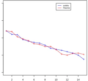
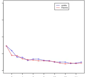
3.7 Real data analysis: Comparison between similarityMix and FlexMix . . . . 32

3.8 Real data analysis: CCU patients . . . 32

3.9 Real data analysis: CSRU patients . . . 33

(14)

3.11 Real data analysis: SICU patients . . . 34

3.12 Real data analysis: TSICU patients . . . 34

4.1 Under Survival Analysis Setting . . . 42

4.2 Survival Model Results . . . 43

4.3 Time-varying AUC for simulated data in Example 1 . . . 48

4.4 Time-varying AUC for simulated data in Example 2 . . . 49

4.5 Time-varying AUC for application to MIMIC III dataset. (a) Ignoring the dependency in censoring (b) Adjusted for dependent censoring . . . 51

5.1 Scenario 1 with independent covariates: left figure plots the change in es-timated coefficients with tuning parameter λ; right figure plots the 10-fold CV MSE vs.λ, the top is showing the number of coefficients that are non-zero. 64 5.2 Scenario 1 with independent covariates: Shows the change in 10-fold CV MSE when the length of the monitoring windows varies . . . 67

5.3 Scenario 2 with independent covariates: Shows the change in 10-fold CV MSE when the length of the monitoring windows varies . . . 68

5.5 Scenario 4 with independent covariates: left figure plots the change in esti-mated coefficients with tuning parameterλ; right figure plots the 10-fold CV MSE vs.λ, the top is showing the number of coefficients that are non-zero. 70 5.6 Scenario 4 with independent covariates: Shows the change in 10-fold CV MSE when the length of the monitoring windows varies . . . 71

(15)

5.8 Scenario 1 with covariates following ARMA (2,1): Shows the change in 10-fold CV MSE when the length of the monitoring windows varies . . . 73

A.1 ACF plot for ARMA (2,1) . . . 91

A.2 ACF plot for an ARMA (3,0) . . . 92

A.3 Scenario 1 with covariates following ARMA (3,0): Shows the change in 10-fold CV MSE when the length of the monitoring windows varies . . . 93

(16)

A.8 ACF plot for ARMA (0,3) . . . 98

(17)

Chapter 1 Introduction

1.1 Statistical Prediction

People are often interested in predicting a new or future observation. In some of the predictions, statistical inference is made from a sample of a population and is generalized to the whole population whose outcome is uncertain or unknown. Predictions can also be made for future outcomes based on history - that is, generalization of a given predictive model into the future. In e-commerce for example, people are interested in predicting what a customer might be interested in buying based on the purchasing histories of other

customers (one example is in Wang 2016 [56]). Image recognition is also a prediction

problem. An example is the identification of hand-written digits (for one example, Niu 2012

[36]). Typically, a training set of images with known digits is used to build a prediction

model. Then the digit of a new hand-written digit picture will be identified according to that model. In clinical decision making, physicians need to know what is the survival likelihood of a patient after getting a heart transplant. It is important to identify the

(18)

differences between association and prediction. Association is usually model dependent, as all models are only an approximation of the truth. Predictions can usually be validated, using a training-test data split for example. A stronger association does not necessarily imply higher prediction power, as association does not necessarily imply causation.

1.1.1 Prediction Models

I will begin with a brief overview of common types of statistical prediction models. The simplest model is a linear regression model where a linear relationship is assumed between

outcomeY and input matrixX. IfY is categorical, a multivariate logistic regression model

can be used where the logit of the probabilities P(Y =y) is linear in X.

In many cases, Y is not linear in X, and a more general way of representing the

relationship is needed. This can be accomplished using more flexible model specifications, for which one example utilizes regression splines. Smoothing splines, a particular form of

penalized spline (e.g., Ruppert , Wand, and Carroll text, 2003 [44]) is another option. This

is done by dividing X into different regions and modelY with polynomials ofX within each

region. The order of the spline, the location and number of the knots need to be specified. Kernel methods are often used as well. Kernel methods estimate the conditional mean using local information. Larger neighborhoods lead to larger bias and smaller variance, and smaller neighborhoods lead to smaller bias and larger variance. Common choices of the kernel includes the Gaussian kernel, the Epanechnikov kernel, and the tri-cube kernel [14].

K-Nearest-Neighbor methods use the k closest neighbors ofx to predict Y, i.e.,

ˆ

Y(x) = 1/k X

xi∈Nk(x)

(19)

whereNk(x) is the k nearest neighborhood ofxand is defined using the Euclidean distance. Tree-based methods partition the feature space into rectangles by splitting a feature variable at each node to maximize some similarity measure within each daughter node. To correct for the over-fitting tendency of a tree, a random forest can be used. A random forest consists of trees with the splitting feature variables selected from a bootstrap sample of all features. The average prediction from all trees are combined to make a final prediction.

[30]. Boosting methods are commonly used as well. It combines the outputs of ”weak”

classifiers to form a strong one [14].

1.1.2 Prediction Performance

The performance of prediction models can be assessed by a variety of measures. In gen-eral, we want to find predictors with low prediction error, high discrimination ability, and

accurate calibration [49]. Often they cannot all be achieved at the same time.

There are two types of statistical predictors, point estimator and probabilistic estimator.

A point estimator ˆY = ˆf(X) is a function of the input covariates and the function is

estimated based on the training data. Probabilistic estimator gives the probabilities that

Y is smaller than a value. If Y is categorical, it gives the probability that Y is equal to

some number, P(Y = a). The accuracy of point estimators is usually measured by loss

functions. Two common choices of the loss functions are the absolute error loss

L(Y,fˆ(x)) =|Y −fˆ(x)|,

and the squared error loss

(20)

IfY is categorical, the 0-1 loss function,

L(Y,Yˆ) =I(Y = ˆY),

whereI is the indicator function, is commonly used. The prediction error is defined as the

expected value over the loss function. For probabilistic estimators, one way of measuring the prediction error is to dichotomize it into different categories based on a subjectively selected threshold and apply the loss function for point estimators.

Sensitivity and specificity can be used to quantify the discriminative power of a prob-abilistic predictor. That is, how many cases with the outcome have a higher predicted probability of getting that outcome. “Higher probability” can be defined as a probability that is greater than any chosen threshold between 0 and 1. The area under the ROC curve eliminates the need to select a threshold subjectively. It summarizes the sensitivity and specificity of a predictor at all thresholds between 0 and 1. In medical diagnostic testing, each point on the ROC curve can be interpreted as “being a conditional probability of a test result from a random diseased subject exceeding that from a random non-diseased

subject” [39]. It can be applied to measure the performance of a survival model as well

[20]. Some newer methods for measuring discriminative ability include variants of the c

statistic for survival models, reclassification tables, net reclassification improvement (NRI), and integrated discrimination improvement (IDI). NRI was later found to have a high false-positive rate, and a statistically significant NRI statistic should not be relied on as sufficient

evidence for improved prediction performance in the evaluation of biomarkers [38].

Calibration can be measured using a goodness of fit test. One example that the three properties cannot be achieved at the same time is, if the data is highly imbalanced between two classes, classification accuracy might be very high for a model that tends to predict the major class for all predictions. Such a model is not useful in practice since it does

(21)

not have any discriminative power. A confusion matrix that display the false-positive and false-negative rates will provide more informative, and an alternative model with higher prediction error but better discriminative ability might have better prediction performance.

1.2 Improving Prediction with Similarity Measure

Traditionally, a global model is fitted to the entire dataset to optimize the average model performance. It is quite possible that the prediction of some subsets of data under the global model does not perform as well. Moreover, if the size of the subset is small, the parameter estimates are dominated by the majority cases. It is possible that this group can be identified using some of the available covariates. If we can use information from the available features to identify this subgroup, and build separate models for them, the resulting model will be more useful for that group, and improves prediction performance

of the overall model as well. This motivates my proposal to define similarity based on

the relationship between the covariates of the outcomes instead of just the closeness of the feature vectors or the outcomes. The idea of using similarity to improve prediction performance can be seen in a number of papers, some discussed in Subsections 1.2.1, 1.2.2, and Sections 2.1 and 2.2. Based on how similarity is defined, these methods can be generally divided into two categories, unsupervised and supervised.

1.2.1 Unsupervised Methods

Liu et al. (2007) [31] applied the similarity-based approach to neural networks. They used

unsupervised clustering to divide sample data into K groups and then trained separately

(22)

for prediction. They showed that when applied to financial time series prediction the method reduced the computation time and the complexity of the model and improved

trend accuracy in prediction. Lowskey et al. (2013) [32] applied similarity to model the

effect of covariates on a survival outcome. Instead of generating one survival curve for the entire training dataset, for a new patient j in the test dataset, their algorithm generates a Kaplan-Meier survival curve based on K-nearest neighbors of that patient in the training set. The Mahalanobis distance between the covariates was used as the similarity measure to find the K-nearest neighbors.

Trivedi, Pardos & Heffernan (2015) [53] investigated the utility of clustering in

improv-ing prediction accuracy, and also provided some explanations on why this approach may increase prediction accuracy. They applied k-means clustering first and then obtained k sets of predictors for each cluster. The k sets of predictions were then combined using a naive ensemble for prediction. When similarity measure is defined in an unsupervised way, it will only depend on the covariates. The relative explanatory ability or the relationship between the covariates and the outcome is ignored.

1.2.2 Supervised and Semi-Supervised Methods

Ishwaran et al. (2008) [22] extended a random forest model to survival outcomes. By

splitting nodes to maximize survival difference, dissimilar cases will end up in different nodes while cases in the same node will be more homogeneous. A cumulative hazard function (CHF) is calculated for each tree and then averaged to obtain the ensemble CHF. As a result, the CHF obtained from similar cases are used to predict the CHF of a new case.

Xu, Nettleton, & Nordman (2014) [57] developed case-specific random forests (CSRFs).

(23)

scheme and generates a global random forest for all cases, Xu, Nettleton, & Nordman

(2014) [57] applied weights to assign higher probabilities to cases that are more similar to

the target case. The similarity is defined using bagging of trees, that is, firstly, a standard RF model is fit to the data. The greater the degree trees group two cases into the same node, the more similar these two cases are. However, the drawback of applying random

forest models, e.g., either Ishwaran et al. (2008) or Xu, Nettleton & Nordman (2014) [57],

to clinical data is computational burden and a lack of interpretability.

1.3 Thesis Outline

Chapter 2 will discuss general prediction problems in clinical settings and especially the challenges of predictions in the ICU. The MIMIC-III (Medical Information Mart for In-tensive Care III) dataset and the motivating study from that dataset will be introduced. In Chapter 3, I will give an interpretable and meaningful definition of neighborhoods and use simulations to show the idea of building localized models to improve prediction. I will propose a new method to estimate similarity in a supervised way. In Chapter 4, I will extend our method to survival analysis where the outcome is the time to occurrence of some event. In Chapter 5, I will quantify the relationship between prediction accuracy and the length of the monitoring window of longitudinal covariates.

(24)

Chapter 2 Clinical Prediction

Clinical prediction models provide physicians with evidence-based decision-making by

esti-mating individual probabilities of risks and benefits [11]. The dataset that we mainly focus

on comes from an observational study. Observational studies are used primarily to identify risk and prognostic factors and in cases where randomized controlled trials would be impos-sible or unethical. They often have lower costs (than clinical trials), greater follow-up time for patients, and include a broader range of patients. It has been shown in recent studies that well-designed observational studies provide results similar to randomized controlled trials[2, 8].

2.1 Overview of Similarity-based Prediction in Medicine

The uptake of Electronic Health Records (EHRs) has generated massive health data sets that are big in volume and diverse in variety. Traditional methods assume that all patients in a given dataset have the same relationship between the outcome and the feature vector,

(25)

and focus on a global model to fit the entire training dataset. However this approach may not be optimal for big health data, and using all patient data in the prediction might only be adding computational burden and decreases prediction accuracy.

It has been shown in previous papers that patient similarities from EHR can be utilized to improve prediction of health risks, and to target medical treatments,. For example, Got-tlieb et al. (2013) used basic patient-specific information gathered at admission, to identify

similar patients and then predicting the eventual discharge diagnoses[17]. Panahiazar et

al. (2015) used EHR information such as medical co-morbidities, lab measurements, ejec-tion fracejec-tion, vital status and demographics to identify similar patients, and subsequently

assign medication plans based on the similarity index [37].

2.2 MIMIC III Database

MIMIC-III is a freely accessible critical care database for 53,423 distinct hospital

admis-sions for adult patients. It is an update to the MIMIC-II database [27,46,45] with added

patients from 2008-2012. Data includes vital signs, medications, diagnostic code, survival

data and high resolution data including lab results and bedside monitoring data [23]. They

can provide rich and diverse information for modeling and prediction but also pose chal-lenges to fast and accurate prediction of outcome of interest. Sun et al. (2015) used localized supervised learning to incorporates expert feedback in defining patient similar-ity, and demonstrated the efficacy of their approach with MIMIC-II data, a precursor to

MIMIC-III[50]. Lee, Maslove & Dubin (2015) [26] showed empirically that using a patient

similarity metric (PSM) to only include a subset of similar patients improves mortality prediction in the MIMIC-II database.

(26)

rich database like MIMIC, and with its large sample size, it is possible to identify similar patients and then effectively reduce the sample size while improving the patient outcome performance.

2.3 An Example of a MIMIC Study

One of the studies based on MIMIC database is an Acute Kidney Injury (AKI) study in the ICU (Intensive Care Unit). Acute kidney injury (AKI) is a sudden episode of kidney

failure or kidney damage that happens within a few hours or a few days [1].There are

various ways to diagnose the onset of AKI, and the most widely adopted definition is an increase in creatinine measurement of 0.3mg/dl or a 50% increase compared to the baseline

measurement within 48 hours [34]. The definitions of the key concepts and variables are

listed as follows:

Basic definitions:

AKI: An increase in creatinine measurement of 0.3mg/dl or 50% compared to ICU

admis-sion value within 48 hours after ICU admisadmis-sion.

AKI onset time: The time when creatinine exceeds the threshold.

Peak creatinine: The highest creatinine value within 24 hours or 48 hours after AKI onset

for AKI patients

Recovery: Return to below 10% above admission value.

Censoring: Neither recovered from AKI nor died before hospital discharge

Creatinine Percentage Increase Definition1: The percentage increase of peak creatinine

within 48 hours compared to admission value. (44.51% of patients have peak creatinine is at AKI onset, 23.39% between 0-24 hours, 32.10% between 24-48 hours)

(27)

Figure 2.1: Percentages of patients that recovered, died or were censored

Creatinine Percentage Increase Definition2: The percentage increase of peak creatinine

within 24 hours compared to admission value. (57.07% peak at AKI onset, 42.93% peak between 0-24 hours)

Creatinine Percentage Increase Definition3: The percentage increase of creatinine at AKI

onset time compared to admission value.

Predictors:

Urine Volume: Total amount in 12 hours just before AKI onset, divided by 12.

Systolic Blood Pressure: Average systolic blood pressurein in 12 hours just before AKI.

Age as a continuous predictor

ICU type: 1-CCU(Coronary Care Unit) 2-CSRU (Cardiac Surgery Recovery Unit) 3-FICU

(Finard Medical Surgical ICU)/MICU (Medical Surgical ICU) 4-SICU (Surgical ICU).

Creatinine Admission: Creatinine at ICU admission.

(28)

In MIMIC-II, 3599 out of 22136 (approximately 16.26%) of ICU patients developed AKI after ICU admission, and Figure 2.1 shows the percentages of recovery, death or discharge from hospital for AKI patients. Previous studies showed that AKI is associated with

increased risk of both the short term and long term mortality among patients [34, 33, 16].

A subset of the patients recovered from AKI during ICU or hospital stay, while others do not recover. Clinicians are interested in predicting which patient will recover from the disease and which ones will not, and in developing personalized treatment plans for each type of patient. We want to identify the variables that have good predictive power for predicting the outcome of the patient diagnosed with AKI.

It is interesting to see that while some patients recover very quickly, others take a much longer time to recover, as shown in Figure 2.1. Thus, we want to consider predicting time to recovery from AKI as opposed to merely predicting a single outcome whether they recovered or not. And we would like to use a similarity approach to improve the time-to-event prediction.

Another challenge is that the nature of the urgency in the ICU requires us to start predicting as soon as possible, in order for medical staff to act quickly. For longitudinal predictors, it is important to know how long should the follow up time be so that we can predict as soon as possible without losing potentially critical follow-up information and deteriorating the accuracy of the prediction. This motivates the method in Chapter 5.

(29)

Chapter 3 Similarity-based Patient Outcome

Prediction for Continuous Data

3.1 Introduction

Traditionally, a global model is fitted to the entire dataset to optimize the average model performance. It is quite possible that the prediction of some subsets of data under the global model does not perform as well. Moreover, if the size of the subset is small, the parameter estimates are dominated by the majority cases. It is possible that this group can be identified using some of the available covariates. If we can use information from the available features to identify subgroups, and build separate models for them, the resulting model should be more useful for that group, and should improve prediction performance of the overall model as well.

The idea of using similarity to improve prediction performance can be seen in a number of papers based on how similarity is defined, these methods can be generally divided into

(30)

two categories, unsupervised and supervised, and are discussed in Chapter 1.

In addition to the similarity-based methods, mixture models are commonly used to

represent the heterogeneity in the data as well. For example, FlexMix [28, 18] is a general

framework for fitting discrete mixtures of regression models using EM algorithm, such that the M-step allows a general specification. Posterior probabilities are used as weights in the mixture of regression models, and need to be estimated. Mixture of experts models have also been used in the literature. These models have experts such as regression functions or classifiers and a gate to soft partition the data into different regions, so that individual experts will specialize on a smaller problem. The experts and the gate are then combined

by a probabilistic model [59].

The rest of the section is organized as follows. In Section 3.2.1, we will explore the rationale behind our similarity-based modeling approach. A novel prediction algorithm is proposed in Section 3.2.2 We will demonstrate the prediction performance of the proposed method through simulations in Section 3.3. The impact of model misspecification is also studied.

In Section 3.4, we apply the method to an intensive care unit (ICU) dataset. In Section 3.5, we will summarize our findings and provide discussions on possible future work.

3.2 Methods

It is quite possible that the mixtures can be identified using a portion of the available covariates. If we can utilize that available information, and build separate models for different subgroups, the resulting model could very well be more useful for that group, and improve prediction performance of the overall model as well. That motivates our idea to

(31)

define similarity based on the relationship between the covariates and outcomes instead of just the closeness of the feature vectors or the outcomes.

3.2.1 Problem Set-up

We will first show how the similarity-based modeling is conducted and the reason that it generally has more accurate prediction than modeling using all data points.

Without loss of generality, assume there is a mixture of two linear models in the dataset.

Denote the dataset [Y,X∗] = {(Yi,Xi,Si), i = 1,2, ..., n}, where Y is a continuous

out-come. The columns of X∗_i consist of columns of Xi and Si, and might have common

elements. The elements in Si are called the similarity variables here and the elements

in Xi are called the regression variables. Consider the following linear regression model:

Yi =Xiβ+iiff(Si)∈(a, b) andYi =Xiα+i otherwise,i= 1,2, ..., n. Yiis the response variable, and Xi = (1, Xi1, Xi2, ..., Xip) is a 1×(p+ 1) vector. β = (β0, β1, ..., βp)T and

α = (α0, α1, ..., αp)T are both vectors of (p+ 1)×1 regression coefficients. f is assumed to be a smooth function of the similarity variables, and maps the similarity variables to a

real number. (a, b) is any open interval on the real line. i is independently and normally

distributed with mean 0 and variance σ2_.

For each case i, i = 1,2, ...n, using some suitable distance measure, such as Euclidean

distance or Mahalanobis distance, a functionD, the distance betweeni, and any other case

j,j = 1,2, ...n,j not equal toi, is denoted asD(Si, Sj). The k cases corresponding to the

smallest distances with i will be called the neighborhood of i. Suppose case i corresponds

to the first linear model, that is, Yi =Xiβ+i, with suitable f, it is fair to assume that

when k is sufficiently small, the neighborhood ofi also corresponds to the same model. So

(32)

of i, which consists only of cases from the same distribution, the model estimates will be unbiased. As we widen the neighborhood, at some point, cases from the second model

Yi = Xiα+ will be included. Fitting an ordinary linear model to all the data in the

widened neighborhood will in general lead to increased mean squared error. Fitting an ordinary linear model to all the data in the widened neighborhood will lead to biased

estimates of ˆY and in general increased mean squared error. We will briefly show the proof

as follows.

Depending onf(Si),i= 1,2, ..., n, partitionXn×(p+1) into two sets, so that Xi = (W_Z),

and Y = W α_Zβ₊+, where W is an n1×(p+ 1) matrix and Z is an n2 ×(p+ 1) matrix

with n1 +n2 = n. By using all the data in the sample, the OLS estimate of Y, is

b

Y =X(XT_X₎−1_XT_Y_{. It is easy to show that} _XT_X ₌_WT_W ₊_ZT_Z_{. Then:}

E( ˆY) = (W Z )(W T W +ZTZ)−1(WTW α+ZTZβ) = (W Z )(W T W +ZTZ)−1(WTW α+ZTZα−ZTZα+ZTZβ) = (W Z )[α−(W T W +ZTZ)−1ZTZ(α−β)]. Thus: E( ˆY)−E(Y)= _Zα₋0_Zβ −(W Z )(W T_W ₊_ZT_Z₎−1_ZT_Z₍_α₋_β₎ = (0 Z)(α−β)−X(X T_X₎−1_ZT_Z₍_α₋_β₎ = [(0 Z)−X(X T_X₎−1_ZT_Z_](_α₋_β₎

We can see that E( ˆY) generally does not equal to E(Y), i.e., the estimated Y is not

unbiased unless the coefficients in the two models are the same.

We will further use simulations from two models, to provide more rationale for

similarity-based predictions. For simplicity, suppose we only have three variables, X1, X2 and

(33)

Figure 3.1: Case 1 data, Y vs. X1, X2,X3 ● ● ● ● ● ● ● ● ● ● ● ● ● ● ● ● ● ● ● ● ● ● ● ● ● ● ● ● ● ● ● ● ● ● ● ● ● ● ● ● ● ● ● ● ● ● ● ● ● ● ● ● ● ● ● ● ● ● ● ● ● ● ● ● ● ● ● ● ● ● ● ● ● ● ● ● ● ● ● ● ● ● ● ● ● ● ● ● ● ● ● ● ● ● ● ● ● ● ● ● ● ● ● ● ● ● ● ● ● ● ● ● ● ● ●● ● ● ● ● ● ● ● ● ● ● ● ● ● ● ● ● ● ● ● ● ● ● ● ● ● ● ● ● ● ● ● ● ● ● ● ● ● ● ● ● ● ● ● ● ● ● ● ● ● ● ● ● ● ● ● ● ● ● ● ● ● ● ●● ● ● ● ● ● ● ● ● ● ● ● ● ● ● ● ● ● ● ● ● ● ● ● ● ● ● ● ● ● ● ● ● ● ● ● ● ● ● ● ● ● ● ● ● ● ● ● ● ● ● ● ● ● ● ● ● ● ● ● ● ● ● ● ● ● ● ● ● ● ● ● ● ● ● ● ● ● ● ● ● ● ● ● ● ● ● ● ● ● ● ● ● ● ● ● ● ● ● ● ● ● ● ● ● ● ● ● ● ● ● ● ● ● ● ● ● ● ● ● ●● ● ● ● ● ● ● ● ● ● ● ● ● ● ● ● ● ● ● ● ● ● ● ● ● ● ● ● ● ● ● ● ● ● ● ● ● ● ● ● ● ● ● ● ● ● ● ● ● ● ● ● ● ● ● ● ● ● ● ● ● ● ● ● ● ●● ● ● ● ● ● ● ● ● ● ● ● ● ● ● ●● ● ● ● ● ● ● ● ● ● ● ● ● ● ● ● ● ● ● ● ● ● ● ● ● ● ● ● ● ● ● ● ● ● ● ● ● ● ● ● ● ● ● ● ● ● ● ● ● ● ● ● ● ● ● ● ● ● ● ● ● ● ● ● ● ● ● ● ● ● ● ● ● ● ● ● ● ● ● ● ● ● ● ● ● ● ● ● ● ● ● ● ● ● ● ● ● ● ● ● ● ● ● ● ● ● ● ● ● ● ● ● ● ● ● ● ● ● ● ● ● ● ● ● ● ● ● ● ● ● ● ● ● ● ● ● ● ● ● ● ● ● ● ● ● ● ● ● ● ● ● ● ● ● ● ● ● ● ● ● ● ● ● ● ● ● ● ● ● ● ● ● ● ● ● ● ● ● ● ● ● ● ● ● ● ● ● ● ● ● ● ● ● ● ● ● ● ● ● ● ● ● ● ● ● ● ● ● ● ● ● ● ● ● ● ● ● ● ● ● ● ● ● ● ● ● ● ● ● ● ● ● ● ● ● ● ● ● ● ● ● ● ● ● ● ● ● ● ● ● ● ● ● ● ● ● ● ● ● ● ● ● ● ● ● ● ● ● ● ● ● ● ● ● ● ● ● ● ● ● ● ● ● ● ● ● ● ● ● ● ● ● ● ● ● ● ● ● ● ● ● ● ● ● ● ● ● ● ● ● ● ● ● ● ● ● ● ● ● ● ● ● ● ● ● ● ● ● ● ● ● ● ● ● ● ●● ● ● ● ● ● ● ● ● ● ● ● ● ● ● ● ● ● ● ● ● ● ● ● ● ● ● ● ● ● ● ● ● ● ● ● ● ● ● ● ● ● ● ● ● ● ● ● ● ● ● ● ● ● ● ● ● ● ● ● ● ● ● ● ● ● ● ● ● ● ● ● ● ● ● ● ● ● ● ● ● ● ● ● ● ● ● ● ● ● ● ● ●● ● ● ● ● ● ● ● ● ● ● ● ● ● ● ● ● ● ● ● ● ● ● ● ● ● ● ● ● ● ● ● ● ● ● ● ● ● ● ● ● ● ● ● ● ● ● ● ● ●● ● ● ● ● ● ● ● ● ● ● ● ● ● ● ● ● ● ● ● ● ● ● ● ● ● ● ● ● ● ● ● ● ● ● ● ● ● ● ● ● ● ● ● ● ● ● ● ● ● ● ● ● ● ● ● ● ● ● ● ● ● ● ● ● ● ● ● ● ● ● ● ● ● ● ● ● ● ● ● ● ● ● ● ● ● ● ● ● ● ● ● ● ● ● ● ● ● ● ● ● ● ● ● ● ● ● ● ● ● ● ● ● ● ● ● ● ● ● ● ● ● ● ● ●● ● ● ● ● ● ● ● ● ● ● ● ● ● −30 −20 −10 0 10 20 30 −30 −20 −10 0 10 20 30 X1 Y ● ● ● ● ● ● ● ● ● ● ● ● ● ● ● ● ● ● ● ● ● ● ● ● ● ● ● ● ● ● ● ● ● ● ● ● ● ● ● ● ● ● ● ● ● ● ● ● ● ● ● ● ● ● ● ● ● ● ● ● ● ● ● ● ● ● ● ● ● ● ● ● ● ● ● ● ● ● ● ● ● ● ● ● ● ● ● ● ● ● ● ● ● ● ● ● ● ● ● ● ● ● ● ● ● ● ● ● ● ● ● ● ● ● ● ● ● ● ● ● ● ● ● ● ● ● ● ● ● ● ● ● ● ● ● ● ● ● ● ● ● ● ● ● ● ● ● ● ● ● ● ● ● ● ● ● ● ● ● ● ● ● ● ● ● ● ● ● ● ● ● ● ● ● ● ● ● ● ●● ● ● ● ● ● ● ● ● ● ● ● ● ● ● ● ● ● ● ● ● ● ● ● ● ● ● ● ● ● ● ● ● ● ● ● ● ● ● ● ● ● ● ● ● ● ● ● ● ● ● ● ● ●● ● ● ● ● ● ● ● ● ●● ● ● ● ● ● ● ● ●● ● ● ● ● ● ● ● ● ● ● ● ● ● ● ● ● ● ● ● ● ● ● ● ● ● ● ● ● ● ● ● ● ● ● ● ● ● ● ● ● ● ● ● ● ● ● ● ● ● ● ● ● ● ● ●● ● ● ● ● ● ● ● ● ● ● ● ● ● ● ● ● ● ● ● ● ● ● ● ● ● ● ● ● ● ● ● ● ● ● ● ● ● ● ● ● ● ● ● ●● ● ● ● ● ● ● ● ● ● ● ● ●● ● ● ● ● ● ● ● ● ● ● ● ● ● ● ● ● ●● ● ● ● ● ● ● ● ● ● ● ● ● ● ● ● ● ● ● ● ● ● ● ● ● ● ● ● ● ● ● ● ● ● ● ● ● ● ● ● ● ● ● ● ● ● ● ● ● ● ● ● ● ● ● ● ● ● ● ● ● ● ● ● ● ● ● ● ● ● ● ● ● ● ● ● ● ● ● ● ● ● ● ● ● ● ● ● ● ● ● ● ● ● ● ● ● ● ● ● ● ● ● ● ● ● ● ● ● ● ● ● ● ● ● ● ● ● ● ● ● ● ● ● ● ● ● ● ● ● ● ● ● ● ● ● ● ● ● ● ● ● ● ● ● ● ● ● ● ● ● ● ● ● ● ● ● ● ● ● ● ● ● ● ● ● ● ● ● ● ● ● ● ● ● ● ● ● ● ● ● ● ● ● ● ● ● ● ● ● ● ● ● ● ● ● ● ● ● ● ● ● ● ● ● ● ● ● ● ● ● ● ● ● ● ● ● ● ● ● ● ● ● ● ● ● ● ● ● ● ● ● ● ● ● ● ● ● ● ● ● ● ● ● ● ● ● ● ● ● ● ● ● ● ● ● ● ● ● ● ● ● ● ● ● ●● ● ● ● ● ● ● ● ● ● ● ● ● ● ● ● ●● ● ● ● ● ● ● ● ● ● ● ● ● ● ● ● ● ● ● ● ● ● ● ● ● ● ● ● ● ● ● ● ● ● ● ● ● ● ● ● ● ● ● ● ● ● ● ● ● ● ● ● ● ● ● ● ● ● ● ● ● ● ● ● ● ● ● ● ● ● ● ● ● ● ● ● ● ● ● ● ● ● ● ● ● ● ● ● ● ● ● ● ● ● ● ● ● ● ●● ● ● ● ● ● ● ● ● ● ● ● ● ● ● ● ● ● ● ● ● ● ● ● ● ● ● ● ● ● ● ● ● ● ● ● ● ● ● ● ● ● ● ● ●● ● ● ● ● ● ● ● ● ● ● ● ● ● ● ● ● ● ● ● ● ● ● ● ● ● ● ● ● ● ● ● ● ● ● ● ● ● ● ● ● ● ● ● ● ● ● ● ● ● ● ● ● ● ● ● ● ● ● ● ● ● ● ● ● ● ● ● ●● ● ● ● ● ● ● ● ● ● ● ● ● ● ● ● ● ●● ● ● ● ● ● ● ● ● ● ● ● ● ● ● ● ●● ● ● ● ● ● ● ● ● ● ● ● ● ● ● ● ● ● ● ● ● ● ● ● ● ● ● ● ● ● ● ● ● ● ● ● ● ● ● ● ● ● ● ● ● ● ● ● ● ● ● ● ● ● ● ● ● ● ● ● ● ● ● ● ● ● ● ● ● ● ● ● ● ● ● ● ● ● ● ● ● ● ● ● ● −30 −20 −10 0 10 20 30 −20 0 20 X2 Y ● ● ● ● ● ● ● ● ● ● ● ● ● ● ● ● ● ● ● ● ● ● ● ● ● ● ● ● ● ● ● ● ● ● ● ● ● ● ● ● ● ● ● ● ● ● ● ● ● ● ● ● ● ● ● ● ● ● ● ● ● ● ● ● ● ● ● ● ● ● ● ● ● ● ● ● ●● ● ● ● ● ● ● ● ● ● ● ● ● ● ● ● ● ● ● ● ● ● ● ● ● ● ● ● ● ● ● ● ● ● ●● ● ● ● ● ● ● ● ● ● ● ● ● ● ● ● ● ● ● ● ● ● ● ● ● ● ● ● ● ● ● ● ● ● ● ● ● ● ● ● ● ● ● ● ● ● ● ● ● ● ● ● ● ● ● ● ● ● ● ● ● ● ● ● ● ● ● ● ● ● ● ● ● ● ● ● ● ● ● ● ● ● ● ● ● ● ● ● ● ● ● ● ● ● ● ● ● ● ● ● ● ● ● ● ● ● ● ● ● ● ● ● ● ● ● ● ● ● ● ● ● ● ● ● ● ● ● ● ● ● ● ● ● ● ● ● ● ● ● ● ● ● ● ● ● ● ● ● ● ● ● ● ● ● ● ● ● ● ● ● ● ● ● ● ● ● ● ● ● ● ● ● ● ● ● ● ● ● ● ● ● ● ● ● ●● ● ●● ● ● ● ● ● ● ● ● ● ● ● ● ● ● ● ● ● ● ● ● ● ● ● ● ● ● ● ● ● ● ● ● ● ● ● ● ● ● ● ● ● ● ● ● ● ● ● ● ● ● ● ● ● ● ● ● ● ● ● ● ● ● ● ● ● ● ● ● ● ● ● ● ● ● ● ● ● ● ● ● ● ● ● ● ● ● ● ● ● ● ● ● ● ● ● ● ● ● ● ● ● ● ● ● ● ● ● ● ● ● ● ● ● ● ● ● ● ● ● ● ● ● ● ● ● ● ● ● ● ● ● ● ● ● ● ● ● ● ● ● ● ● ● ● ● ● ● ● ● ● ● ● ● ● ● ● ● ● ● ● ● ● ● ● ● ● ● ● ● ● ● ●● ● ● ● ● ● ● ● ● ● ● ● ● ● ● ● ● ● ● ● ● ● ● ● ● ● ● ● ● ● ● ● ● ● ● ● ● ● ● ● ● ● ● ● ● ● ● ● ● ● ● ● ● ● ● ● ● ● ● ● ● ● ● ● ● ● ● ● ● ● ● ● ● ● ●● ● ● ● ● ● ● ● ● ● ● ● ● ● ● ● ● ● ● ● ● ● ● ● ● ● ● ● ● ● ● ● ● ● ● ● ● ● ● ● ● ● ● ● ● ● ● ● ● ● ● ● ● ● ● ● ● ● ● ● ● ● ● ● ● ● ● ● ● ● ● ● ● ● ● ● ● ● ● ● ● ● ● ● ● ● ● ● ● ● ● ● ● ● ● ● ● ● ● ● ● ●● ● ● ● ● ● ● ● ● ● ● ● ● ● ● ● ● ● ●● ● ● ● ●● ● ● ● ● ● ● ● ● ● ● ● ● ● ● ● ● ● ● ● ● ● ● ● ● ● ● ● ● ● ● ● ● ● ● ● ● ● ● ● ● ● ● ● ● ● ● ● ● ● ● ● ● ● ● ● ● ● ● ● ● ● ● ● ● ● ● ● ● ● ● ● ● ● ● ● ● ● ● ● ● ● ● ● ● ● ● ● ● ● ● ● ● ● ● ● ● ● ● ● ● ● ● ● ● ● ● ● ● ● ● ● ● ● ● ● ● ● ● ● ● ● ● ● ● ● ● ● ● ● ● ● ● ● ● ● ● ● ● ● ● ● ● ● ● ● ● ● ● ● ● ● ● ● ● ● ● ● ● ● ● ● ● ● ● ● ● ● ● ● ● ● ● ● ● ● ● ● ● ● ● ● ● ● ● ● ● ● ● ● ● ● ● ● ● ● ● ● ● ● ● ● ● ● ● ● ● ● ● ● ● ● ● ● ● ● ● ● ● ● ● ● ● ● ● ● ● ● ● ● ● ● ● ● ● ● ● ● ● ● ● ● ● ● ● ● ● ● ● ● ● ● ● ● ● ● ● ● ● ● ● ● ● ● ● ● ● ● ● ● ● ● ● ● ● ● ● ● ● ● ● ● ● ● ● ● ● ● ● ● ● ● ● ● ● ● ● ● ● ● ● ● ● ● ● ● ● ● ● ● ● ● ● ● ● ● ● ● ● ● ● ● ● ● ● ● −30 −20 −10 0 10 20 30 −20 0 20 X3 Y

A = {(a, b)|(a −7)(b + 10) > 0} and IA(Xi1, Xi3) = 1 if (Xi1, Xi3) ∈ A and 0

other-wise. The following set of simulation cases are for proof of concept purposes, as certainly for big datasets, the scope of the problem, both for sample size, and covariate space, will be much larger, in general. Consider the first model:

Yi = (1−IA(Xi1, Xi3))(0.5Xi2−6) +IA(Xi1, Xi3)(0.3Xi2+ 6) +i,

Thus, Y is a continuous mixture, linearly dependent on continuous variable X2 and the

resulting multiplicative interaction between continuous variablesX1 and X3. We

indepen-dently generate (Xi1, Xi2, Xi3) from a normal distribution with mean 0 and variance 102,

and the error termsi are generated from a normal distribution with mean 0 and variance

22. Since pairwise distances need to be calculated, to reduce the computational burden in

the simulation study, and without loss of generality, the sample size n is set to be 1000.

Figure3.1 shows the univariate association between the outcome Y and each variable X1,

X2 and X3. Just viewing the plots, it appears thatX1 andX3 are not very correlated with

the outcome Y. But in fact, they jointly affect the relationship between X2 and Y. For

each sample case j, the distance between j and all other (n−1) cases are calculated and

thek closest cases are selected to train the case j specific model ˆY =β1X1+β2X2+β3X3;

this model is then used to make a prediction for case j. After iterating through all cases,

(34)

Figure 3.2: Case 1 results, average residual sum of squares as the number of similar cases increases 0 10 20 30 40 50 0 250 500 750

Number of Similar Cases

A v er age RSS Similarity Variable X1 X2 X3 X1_X2 X1_X3 X2_X3 X1_X2_X3

Comparison of Model Performance

performance of the prediction.

The combination ofX1 andX3 is the correct similarity measure in this model. But

sup-pose it is unknown which variable(s) define the similarity, and we use Euclidean distances

based on different combinations of X1, X2, X3 to calculate the distance. For example, if

we choose X1 and X2 as the similarity variables, then the distance between case i and

j is Distance(i, j) = D{X1,X2}(i, j) = p

(Xi1−Xj1)2+ (Xi2−Xj2)2. With three

vari-ables, there are seven ways to define distance, i.e., D{X1}(i, j), D{X2}(i, j), D{X3}(i, j),

D{X1,X2}(i, j), D{X1,X3}(i, j), D{X2,X3}(i, j), and D{X1,X2,X3}(i, j). Pairwise distances are

calculated for each case, and the closest k neighbors are then selected for model training. The performance of seven models using different definitions of similarity will be compared.

By increasing the neighborhood size, i.e., increasing k, the performance also varies. As k

(35)

Figure 3.3: Case 2 data, Y vs. X1, X2,X3 ● ● ● ● ● ●● ● ● ● ● ● ● ● ● ● ● ● ● ● ● ● ● ● ● ● ● ● ● ● ● ● ● ● ● ● ● ● ● ● ● ● ● ● ● ● ● ● ● ● ● ● ● ● ● ● ● ● ● ● ● ● ● ● ● ● ● ● ●● ● ● ● ● ● ● ● ● ● ● ● ● ● ● ● ● ● ● ● ● ● ● ● ● ● ● ● ● ● ● ● ● ● ● ● ● ● ● ● ● ● ● ● ● ● ● ● ● ● ● ● ● ● ● ● ● ● ● ● ● ● ● ● ● ● ● ● ● ● ● ● ● ● ● ● ● ● ● ● ● ● ● ● ● ●● ● ● ● ● ● ● ● ● ● ● ● ● ● ● ● ● ● ● ● ● ● ● ● ● ● ● ● ● ● ● ● ● ●● ● ● ● ● ● ● ● ● ● ● ● ● ● ● ● ● ● ● ● ● ● ● ● ● ● ● ● ● ● ● ● ● ● ● ● ● ● ● ● ● ● ● ● ● ● ● ● ● ● ● ● ● ● ● ● ● ● ● ● ● ● ● ● ● ● ● ● ● ● ● ● ● ● ● ● ● ● ● ● ● ● ● ● ● ● ● ● ● ● ● ● ● ● ● ● ● ● ● ● ● ● ● ● ● ● ● ● ● ● ● ● ● ● ● ● ● ● ● ● ● ● ● ● ● ● ● ● ● ● ● ● ● ● ● ● ● ● ● ● ● ● ● ● ● ● ● ● ● ● ● ● ● ● ● ● ● ● ● ● ● ● ● ● ● ● ● ● ● ● ● ● ● ● ● ● ● ● ● ● ● ● ● ● ● ● ● ● ● ● ● ● ● ● ● ● ● ● ● ● ● ● ● ● ● ● ● ● ● ● ● ● ● ● ● ● ● ● ● ● ● ● ● ● ● ● ● ● ● ● ● ● ● ● ● ● ● ● ● ● ● ● ● ● ● ● ● ● ● ● ● ● ● ● ● ● ● ● ● ● ● ● ● ● ● ● ● ● ● ● ● ● ● ● ● ● ● ● ● ● ● ● ● ● ● ● ● ● ● ● ● ● ● ● ● ● ● ● ● ● ● ● ● ● ● ● ● ● ● ● ● ● ● ● ● ● ● ● ● ● ● ● ● ● ● ● ● ● ● ● ● ● ● ● ● ● ● ● ● ● ● ● ● ● ● ● ● ● ● ● ● ● ● ● ● ● ● ● ● ● ● ● ● ● ● ● ● ● ● ● ● ● ● ● ● ● ● ● ● ● ● ● ● ● ● ● ● ● ● ● ● ● ● ● ● ● ● ● ● ● ● ● ● ● ● ● ● ● ● ● ● ● ● ● ● ● ● ● ● ● ● ● ● ● ● ● ● ● ● ● ● ● ● ● ● ● ● ● ● ● ●● ● ● ● ● ● ● ● ● ● ● ● ● ● ● ● ● ● ● ● ● ● ● ● ● ● ● ● ● ● ● ● ● ● ● ● ● ● ● ● ● ● ● ● ● ● ● ● ● ● ● ● ● ● ● ● ● ● ● ● ● ● ● ● ● ● ● ● ● ● ● ● ● ● ● ● ● ● ● ● ● ● ● ● ● ● ● ● ● ● ● ● ● ● ● ● ● ● ● ● ● ● ● ● ● ● ●● ● ● ● ● ● ● ● ● ● ● ● ● ● ● ● ● ● ● ● ● ● ● ● ● ● ●● ● ● ● ● ● ● ● ● ● ● ● ● ● ● ● ● ● ● ● ● ● ● ● ● ● ● ● ● ● ● ● ● ● ● ● ● ● ● ● ● ● ● ● ● ● ● ● ● ● ● ● ● ● ● ● ● ● ● ● ● ● ● ● ● ● ● ● ● ● ● ● ●● ● ● ● ● ● ● ● ● ● ● ● ● ● ● ● ● ● ● ● ● ● ● ● ● ● ● ● ● ● ● ● ● ● ● ● ● ● ● ● ● ● ● ● ● ● ● ● ● ● ● ● ● ● ● ● ● ● ● ● ● ● ● ● ● ● ● ● ● ● ● ● ● ● ● ● ● ● ● ● ● ● ● ● ● ● ● ● ● ● ● ● ● ● ● ● ● ● ● ● ● ● ● ● ● ● ● ● ● ● ● ● ● ● ● ● ● ● ● ● ● ● ● ● ● ● ● ● ● ● ● ● ● ● ● ● ● ● ● ● ● ● ● ● ● ● ● ● ● ● ● ● ● ● ● ● ● ● ● ● ● ● ● −30 −20 −10 0 10 20 30 −20 0 20 X1 Y ● ● ● ● ● ●● ● ● ● ● ● ● ● ● ● ● ● ● ● ● ● ● ● ● ● ● ● ● ● ● ● ● ● ● ● ● ● ● ● ● ● ● ● ● ● ● ● ● ● ● ● ● ● ● ● ● ● ● ● ● ● ● ●● ● ● ● ● ● ● ● ● ● ● ● ● ● ● ● ● ● ● ● ● ● ● ● ●● ● ● ● ● ● ● ● ● ● ● ● ● ● ● ● ● ● ● ● ● ● ● ● ● ● ● ● ● ● ● ● ●● ● ● ● ● ● ● ● ● ● ● ● ● ● ● ● ● ● ● ● ● ● ● ● ● ● ● ● ● ● ● ● ●● ● ● ● ● ● ● ● ● ● ● ● ● ● ● ● ● ● ● ● ● ● ● ● ● ● ● ● ● ● ● ● ● ● ● ● ● ● ● ● ● ● ● ● ● ● ● ● ● ● ● ● ● ● ● ● ● ● ● ● ● ● ● ● ● ● ● ● ● ● ● ● ● ● ● ● ● ● ● ● ● ● ● ● ● ● ● ● ● ● ● ● ● ● ● ● ● ● ● ● ● ● ● ● ● ● ● ● ● ● ● ● ● ● ● ● ● ● ● ● ● ● ● ● ● ● ● ● ● ● ● ● ● ● ● ● ● ● ● ● ● ● ● ● ● ● ● ● ● ● ● ● ● ● ● ● ● ● ● ● ● ● ● ● ● ● ● ● ● ● ● ● ● ● ● ● ● ● ● ● ● ● ● ● ● ● ● ● ● ● ● ● ● ● ● ● ● ●● ● ● ● ● ● ● ● ● ● ● ● ● ● ● ● ● ●● ● ● ● ● ● ● ● ● ● ● ● ● ● ● ● ● ● ● ● ● ● ● ● ● ● ● ● ● ● ● ● ● ● ● ● ● ● ● ● ● ● ● ● ● ● ● ● ● ● ● ● ● ● ● ● ● ● ● ● ● ● ● ● ● ● ● ● ● ● ● ● ● ● ● ● ● ● ● ● ● ● ● ● ● ● ● ● ● ● ● ● ● ● ● ● ● ● ● ● ● ● ● ● ● ● ● ● ● ● ● ● ● ● ● ● ● ● ● ● ● ● ● ● ● ● ● ● ● ● ● ● ● ● ● ● ● ● ● ● ● ● ● ● ● ● ● ● ● ● ● ● ● ● ● ● ● ● ● ● ● ● ● ● ● ● ● ● ● ● ● ● ● ● ● ● ● ● ● ● ● ● ● ● ● ● ● ● ● ● ● ● ● ● ● ● ● ● ● ● ● ● ● ● ● ● ● ● ● ● ● ● ● ● ● ● ● ● ● ● ● ● ● ● ● ● ● ● ● ● ● ● ● ● ● ● ● ● ● ● ● ● ● ● ● ● ● ● ● ● ● ● ● ● ● ● ● ●●● ● ● ● ● ● ● ● ● ● ● ● ● ● ● ● ● ● ● ● ● ● ● ● ● ● ● ● ● ● ● ● ● ● ● ● ● ● ● ● ● ● ● ● ● ● ● ● ● ● ● ● ● ● ● ● ● ● ● ● ● ● ● ● ● ● ● ● ● ● ● ● ● ● ● ● ● ● ● ● ● ● ● ● ● ● ● ● ● ● ● ● ● ● ● ● ● ● ● ● ● ● ● ● ● ● ● ● ● ● ● ● ● ● ● ● ● ● ● ● ● ● ● ● ● ● ● ● ● ● ● ● ● ●● ● ● ● ● ● ● ● ● ● ● ●● ● ● ● ● ● ● ● ● ● ● ● ● ● ● ● ● ● ● ● ● ● ● ● ● ● ● ● ● ● ● ● ● ● ● ● ● ● ● ● ● ● ● ● ● ● ● ● ● ● ● ● ● ● ● ● ● ● ● ● ●● ● ● ● ● ● ● ● ● ● ● ● ● ● ● ● ● ● ● ● ● ● ● ● ● ● ● ● ● ● ● ● ● ● ● ● ● ● ● ● ● ● ● ● ● ● ● ● ● ● ● ● ● ● ● ● ● ● ● ● ● ● ● ● ● ● ● ● ● ● ● ● ● ● ● ● ● ● ● ● ● ● ● ● ● ● ● ● ● ● ● ● ● ● ● ● ● ● ● ● ● ● ● ● ● ● ● ● ● ● ● ● ● ● ● ● ● ● ● ● ● ● ● ● ● ● ● ● ● ● ● ● ● ● ● ● ● ● ● ● ● ● ●● ●● ● ● ● ● ● ● ● ● ● ● ● ● ● ● ● ● ● −30 −20 −10 0 10 20 30 −20 0 20 X2 Y ● ● ● ● ● ● ● ● ● ● ● ● ● ● ● ● ● ● ● ● ● ● ● ● ● ● ● ● ● ● ● ● ● ● ● ● ● ● ● ● ● ● ● ● ● ● ● ● ● ● ● ● ● ● ● ● ● ● ● ● ● ● ● ● ● ● ● ● ●● ● ● ● ● ● ● ● ● ● ● ● ● ● ● ● ● ● ● ● ● ● ● ● ● ● ● ● ● ● ● ● ● ● ● ● ● ● ● ● ● ● ● ● ● ● ● ● ● ● ● ● ● ● ● ● ● ● ● ● ● ● ● ● ● ● ● ● ● ● ● ● ● ● ● ● ● ● ● ● ● ● ● ● ● ● ● ● ● ● ● ● ● ● ● ● ● ● ● ● ● ● ● ● ● ● ● ● ● ● ● ● ● ● ● ● ● ● ● ● ● ● ● ● ● ● ● ● ● ● ● ● ● ● ● ● ● ● ● ● ● ● ● ● ● ● ● ● ● ● ● ● ● ● ● ● ● ● ● ● ● ● ● ● ● ● ● ● ● ● ● ● ● ● ● ● ● ● ● ● ● ● ● ● ● ● ● ● ● ● ● ● ● ● ● ● ● ● ● ● ● ● ● ● ● ● ● ● ● ● ● ● ● ● ● ● ● ● ● ● ● ● ● ● ● ● ● ● ● ● ● ● ● ● ● ● ● ● ● ● ● ● ● ● ● ● ● ● ● ● ● ● ● ● ● ● ● ● ● ● ● ● ● ● ● ● ● ● ● ● ● ● ● ● ● ● ● ● ● ● ● ● ● ● ● ● ● ● ● ● ● ● ● ● ● ● ● ● ● ● ● ● ● ● ● ● ● ● ● ● ● ● ● ● ● ● ● ● ● ● ● ● ● ● ● ● ● ● ● ● ● ● ● ● ● ● ● ● ● ● ● ● ● ● ● ● ● ● ● ● ● ● ● ● ● ● ● ● ● ● ● ● ● ● ● ● ● ● ● ● ● ● ● ● ● ● ● ● ● ● ● ● ● ● ● ● ● ● ● ● ● ● ● ● ● ● ● ● ● ● ● ● ● ● ● ● ● ● ● ● ● ● ● ● ● ● ● ● ● ● ● ● ● ● ● ● ● ● ● ● ● ● ● ● ● ● ● ● ● ● ● ● ● ● ● ● ● ● ● ● ● ● ● ● ● ● ● ● ● ● ● ● ● ● ● ● ● ● ● ● ● ● ● ● ● ● ● ● ● ● ● ● ● ● ● ● ● ● ● ● ● ● ● ● ● ● ● ● ● ● ● ● ● ● ● ● ● ● ● ● ● ● ● ● ● ● ● ● ● ● ● ● ● ● ● ● ● ● ● ● ● ● ● ● ● ● ● ● ● ● ● ● ● ● ● ● ● ● ● ● ● ● ● ● ● ● ● ● ● ●●● ● ● ● ● ● ● ● ● ● ● ● ● ● ● ● ● ● ● ● ● ● ● ● ● ● ● ● ● ● ● ● ● ● ● ● ● ● ● ● ● ● ● ● ● ● ● ● ● ● ● ● ● ● ● ● ● ● ● ● ● ● ● ● ● ● ● ● ● ● ● ● ● ● ● ● ● ● ● ● ● ● ● ● ● ● ● ● ● ● ● ● ● ● ● ● ● ● ● ● ● ● ● ● ● ● ● ● ● ● ● ● ● ● ● ● ● ● ● ● ● ● ● ● ● ● ● ● ● ● ● ● ● ● ● ● ● ● ● ● ● ● ● ● ● ● ● ● ● ● ● ● ● ● ● ● ● ● ● ● ● ● ● ● ● ● ● ● ● ● ● ● ● ● ● ● ● ● ● ● ● ● ● ● ● ● ● ● ● ● ● ● ● ● ● ● ● ● ● ● ● ● ● ● ● ● ● ● ● ● ● ● ● ● ● ● ● ● ● ● ● ● ● ● ● ● ● ● ● ● ● ● ● ● ● ● ● ●● ● ● ● ● ● ● ● ● ● ● ● ● ● ● ● ● ● ● ● ● ● ● ● ● ● ● ● ● ● ● ● ● ● ● ● ● ● ● ● ● ● ● ● ● ● ● ● ● ● ● ● ● ● ● ● ● ● ● ● ● ● ● ● ● ● ●● ● ● ● ● ● ● ● ● ● ● ● ● ● ● ● ● ● ● ● ● ● ● ● ● ● ● ● ● ● ● ● ● ● ● ● ● ● ● ● ● ● ● ● ●● ● ● ● ● ● ● ● ● ● ● ● ● ● ● ● ● ● ● ● −30 −20 −10 0 10 20 30 −30 −20 −10 0 10 20 30 X3 Y

model using all the sample points. The above simulation is repeated 100 times to obtain an averaged residual sum of squares.

As shown in Figure 3.2, as k increases, the performances of all seven models converge.

When k is very small, the model performance deteriorates due to small sample size and

resulting variability issues. The RSS curve shows a skewed U-shape except when X2

was chosen. The residual sum of squares is the smallest when both correct variables for

similarity are chosen, that is, when bothX1 andX3 are used in calculation of the distance,

and the neighborhood is sufficiently small to exclude less relevant cases. The second best

case is when all of the variables are used. If the wrong similarity variable X2 is the only

similarity variable used, the performance is the worst among all other scenarios. Also, if only one of the correct similarity variables is picked, the performance is not much improved, since the two similarity variables jointly affect the neighborhood.

For the second model,

Yi =(1−IA(Xi1, Xi3))(0.3Xi1+ 0.5Xi2 + 0.1Xi3 −6)

+IA(Xi1, Xi3)(0.7Xi1+ 0.3Xi2−0.1Xi3+ 6) +i,

whereA={(a, b)|(a−7)(b+ 10)>0}. X1, X2, X3 are normally distributed with mean 0

and variance 102_{, and the error term is normally distributed with mean 0 and variance 2}2_.

(36)

onlyX2 is in the linear component is that in this case all three variables are in the linear

component. Figure3.3 shows the plots ofY against each of the three variables. Unlike in

Case 1 where X1 and X3 appear to be uncorrelated with Y, here there is a linear trend

between the two variables and Y. This simulation tries to investigate the behavior of the similarity-based modeling when the similarity variable is also in the regression component.

Patterns analogous to those seen in Case 1 can also been seen here. Figure 3.4 shows

that when the correct similarity variables are selected, the lowest averaged residual sum of squares is achieved, when compared both horizontally and vertically. Using all the variables as similarity variables, the model performance is better than choosing only one correct similarity variable, but worse than when choosing two correct ones. Again we can see the U-shape of RSS curve just as in Case 1, which we speculate is due to when the sample size is very small, increasing the neighborhood includes more cases of the same class without introducing too many dissimilar cases, and the increase of similar cases reduces the additional variability from sample size that could take the prediction off target.

3.2.2 Algorithm

The previous two examples showed the importance of identifying similarity variables in localized prediction.

In this section, we will propose a new method to find similarity variables, and utilize that information to improve prediction.

We will call it similarityMix. Suppose there are n individuals and K mixture

compo-nents. Let Yi = K X j=1 If(Si)=j(Xiβj) +i, i= 1,2, ..., n

(37)

Figure 3.4: Case 2 results, average residual sum of squares as the number of similar cases increases 0 10 20 30 40 50 0 250 500 750

Number of Similar Cases

A v er age RSS Similarity Variables X1 X2 X3 X1_X2 X1_X3 X2_X3 X1_X2_X3

Comparison of Model Performance

wherei, i= 1,2, ..., nare i.i.d Gaussian (0, σ2). f(Si) takes value in 1,2, ..., K andIf(Si)=j

equals 1 iff(Si) =j and 0 otherwise. Xi stands for regression variables andSi stands for

similarity variables for individuali. β_jare the regression coefficients for mixture component

j, j = 1, ..., K. Let Y = [Y1, Y2, ...Yn]0, X = [X10,X20, ...Xn0]0, and S = [S10,S20, ...Sn0]0.

LetZ =X∪S be the set of all variables. Then the likelihood is,

L(Y|X,β₁, ...,β_K, f,S) = K Y j=1 n Y i=1 N(Yi|Xi,βj, σ2)If(S)=j,

where N(Yi|Xi,βj, σ2) is the density for a Gaussian distribution with mean Xiβj and

varianceσ2_{. And the log-likelihood is}

logL(Y|X,β₁, ...,β_K, f,S) = K X j=1 n X i=1 If(S)=jlog(N(Yi|Xi,βj, σ 2₎₎ .

(38)

The main difference between this model and the mixture of experts model is that a hard threshold, represented by an indicator function, is used here, and the algorithm is a combi-nation of an EM type algorithm and an additional step of fitting similarity variables (Step 5).

The algorithm is as follows,

1. f(Si), i= 1,2, ..., n is the initial guess for mixture assignment. For t=0 to T,

2. Given f(Si)t=0, i = 1,2, ..., n, maximize the likelihood for each mixture j to get the

regression coefficients ˆβ_jt. In this step, we will use all variables in Z asX for now.

3. Given ˆβ_jt, for i=1,2,...,n, update f(Si)t to f(Si)t+1 to maximize the likelihood. That

is, ˆf(Si)t+1 = arg minj(Yi−βˆj t

Xi)2.

4. Repeat Step 2 and 3 until convergence of the respective coefficients.

5. After getting estimates for ˆβ_j, j = 1,2, ..., K, and ˆf(Si), i= 1,2, ..., n, the next step is to

determine similarity variablesS and the relationship between the similarity variables and

group assignmentsf. We first fit a multinomial logistic regression with ˆf(Si), i= 1,2, ..., n

as the outcome and all variables in Z as covariates. To select the similarity variables,

standard variable selecting techniques for logistic regressions can be used. Tree structures such as classification/decision trees can be used to fit the similarity component as well. For prediction, a new case will be assigned to one of the components using similarity variables, then the model for that component will be used for prediction.

(39)

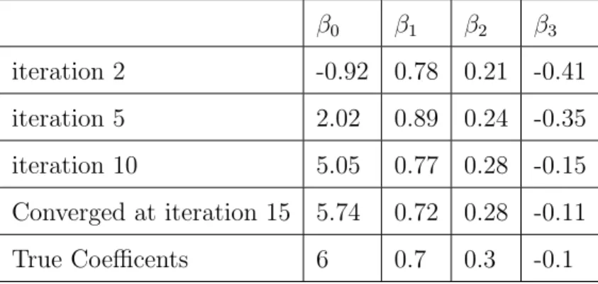
Table 3.1: Estimated coefficients for mixture 1 in Case 1 β0 β1 β2 β3 iteration 2 -0.92 0.78 0.21 -0.41 iteration 5 2.02 0.89 0.24 -0.35 iteration 10 5.05 0.77 0.28 -0.15 Converged at iteration 15 5.74 0.72 0.28 -0.11 True Coefficents 6 0.7 0.3 -0.1

3.3 Simulation Studies

3.3.1 Mixture of Two First-order Polynomials

In the first example, I will look into the convergence of similarityMix whenY is a mixture

of two first-order polynomials, i.e.

Yi =(1−IA(Xi1, Xi3))(0.3Xi1+ 0.5Xi2 + 0.1Xi3 −6)

+IA(Xi1, Xi3)(0.7Xi1+ 0.3Xi2−0.1Xi3+ 6) +i,

(3.1)

where A= {(a, b)|(a−7)(b+ 10) >0}. n = 1000 sample points are generated where X1,

X2, X3 ∼ i.i.d. Gaussian(0,10), and the error terms ∼ i.i.d Gaussian(0,2). The updates

of class assignments and the fitted regression curves at each iteration are studied when we

apply the first step of the proposed algorithm. Figure 3.5 plots the class assignments of

each data point from X2 perspective at iteration 2, 5, 10 and 15. Table 3.1 and 3.2 show

that the regression curves converges quickly to the true regression curves. The algorithm converges at the 15th iteration.

New Methods for Improving Accuracy in Three Distinct Predictive Modeling Problems