Optimizations In Compiler: Vectorization, Reordering, Register Allocation And Verification Of Explicitly Parallel Programs

(1)

Optimizations In Compiler: Vectorization,

Reordering, Register Allocation And Verification

Of Explicitly Parallel Programs

Santanu Das

A Thesis Submitted to

Indian Institute of Technology Hyderabad In Partial Fulfillment of the Requirements for

The Degree of Master of Technology

Department of Computer Science and Engineering

(2)

(3)

(4)

Acknowledgements

I would like to express my gratitude to my thesis advisor Dr. Ramakrishna Upadrasta for continuous encouragement and support during my entire duration of M.Tech Thesis. I have grown both technically and personally since I joined the program. I also acquired the right direction and attitude required for research from him. I sincerely thank him for giving me opportunity to be part of industry as an intern which allowed me to expand my knowhow.

I express my sincere thanks to my thesis committee membersDr. Saurabh Joshi,Dr. M.V. Panduranga Raoand Dr. Subrahmanyam Kalyanasundaramand Dr. Sparsh Mittalfor critical suggestions and feedback.

I would also like to thank my compiler group teammates for their support during my stay at IIT Hyderabad. My heartfelt thanks to my lab mates Abhishek, Anirudh, Gayatri, Shalini, Tharun,UtpalandVenkat. I would definitely miss our fun activities and intelligent discussions. I extend my special thanks to Utpal for his mentorship and guidance.

(5)

Dedication

(6)

Abstract

Compiler Optimizations form a very important part of compiler development as they make a major difference between an average and a great compiler. There are various modules of a compiler-which opens opportunities for optimizations on various spheres. In this thesis, a comparative study of vectorization is done exposing the strengths and weaknesses of various contemporary compilers. Additionally, a study on the impact of vectorization on tiled code is performed. Different strategies for loop nest optimization is explored. An algorithm for statement reordering in loops to enhance performance has been developed. An Integer Linear Program formulation is done to improve loop parallelism, which makes use of loop unrolling and explicitly parallel directives. Finally, an attempt for optimal loop distribution is made. Following loop nest optimization chapter, an explanation of interprocedural register allocation(IPRA) for ARM32 and AArch64 is given. Additionally, a brief description of the problems for implementing IPRA for those architectures is presented. We conclude the chapter with the performance results with IPRA for those platforms. In the last chapter, a description of VoPiL, a static OpenMP verifier in LLVM, is presented. A brief description of the analysis and the results are included.

(7)

Introduction

In the thesis, we explore, study and improve various aspects of LLVM compiler. The topics covered in the thesis are briefly mentioned below.

1.1 A Comparative Study of Vectorization in Compilers

In the second chapter, we make a study of vectorization in LLVM and compare it with other relevant compilers. We benchmark on various vectorization related benchmarks to get a clear idea about the state of vectorization and the scope of improvement. This study exposes the various strengths as also the weaknesses and bottlenecks to vectorization. We comparatively present the number of loops successfully vectorized by the competing compilers. Additionally, We compare the performance improvement due to vectorization over the serial codes.

1.2 A Short Study of Vectorization on Tiled Code

In the following chapter we analyze the impact of vectorization on tiled codes. We represent the improvement or degradation of performance for various permutations of optimizations like tiling, loop transformations and vectorization to find the right optimization sequence which gives the best result.

1.3 Loop Nest Optimization

In the third chapter we present various loop nest optimization techniques that improve the perfor-mance of loop structures. We apply a technique of statement reordering the expose vectorization in a loop nest. We benchmark it on popular benchmark to find performance improvements. We also develop a novel technique to use loop unrolling and explicitly parallel program directives to expose parallelism in a loop. Lastly, we present a dynamic programming technique for improving loop distribution in a loop nest.

(10)

1.4 Interprocedural Register Allocation in LLVM for ARM32/AArch64

In the following chapter, we develop support for Interprocedural Register Allocation for ARM32 and

AArch64 architectures in LLVM compiler. We discuss various problems faced and their workarounds. Finally we present the results in terms of performance gain and code size reduction.

1.5 VoPiL: Verification of OpenMP programs in LLVM

Last but not the least, we develop a static OpenMP verifier in LLVM which verifies the source code programmer supplied explicitly parallel program directives. We test out the efficacy of the tool build over LLVM in a benchmark containing kernels with and without dataraces. Additionally, we compare our tool with other contemporary datarace detection tools.

(11)

Chapter 2

A Comparative Study of

Vectorization in Compilers

2.1 Introduction to Vectorization

SIMD vectorization is a parallelization scheme which uses hardware features like SSE, FMA and AVX along with compiler support. For this purpose, various wide registers have been added to the architecture. These registers have greater length (128, 256 or 512 bits) than regular registers to load multiple data units into them, and then perform an operation simultaneously. These registers have special Load-Store Units which support multiple load/stores in a single cycle and have separate ALU for vector computation. In this chapter, we deal with loop vectorization, ie. vectorization of statements in the loop body. Our work focuses on a type of SIMD vectorization: the problem of automatic vectorization of programs within the compiler framework which makes use of supporting hardware architectures like Streaming SIMD Extensions (SSE).

In this chapter, we present a detailed analysis and comparison of three compilers: LLVM, GCC and ICC (Intel Compiler). We focus on their strengths and weaknesses. We used three benchmarks for the analysis: TSVC, TORCH and MiBench.

2.2 Related Work

A similar comparison has been made in the past. Maliki et. al [1] . This paper evaluates how well compilers vectorize a synthetic benchmark named TSVC [2], consisting of 151 loops.Along with it, two application from Petascale Application Collaboration Teams (PACT), and eight applications from Media Bench II have also been evaluated. The latter two benchmarks are not synthetic in nature. Three compilers: GCC (version 4.7.0), ICC (version 12.0) and XLC (version 11.01) have been evaluated on their capability in vectorization. The results obtained were surprising. Despite long years of research and application, many loops which should be vectorized are not done. Out study is an extension to this study, on more recent compiler versions and also, on more real world benchmarks which are used extensively.

(12)

2.3 Description

In this chapter, we present a detailed analysis and comparison of three compilers: LLVM v3.9, GCC v5.0.3 and ICC(Intel Compiler) v16.0.3 highlighting their strengths and exposing weaknesses com-paratively. We have used three benchmarks for the analysis: TSVC [2], TORCH [3] and MiBench [4]. TSVC is a synthetic benchmark consisting of 151 loops; TORCH and MiBench are real-world bench-marks consisting of computationally intensive codes. We briefly describe each of them below.

• The TSVC suite was originally written in Fortran and later compiled to C. It contains a set of microkernels which test the vectorization capability of the compiler. It contains testing various scenarios which may require loop transformations. The various transformations will be described in the sections below.

• The MiBench suite was developed by Guthais et al [2]. It is a benchmark suite which consists of real-world application programs from six categories: Control, Network, Security, Consumer, Office and Telecommunications.

• The TORCH suite was developed by Kaiser et al. It is a set of computational reference kernels for computer science research. It contains program kernels from the domain of linear algebra, graph theory, n-body simulations, sorting and spectral methods.

2.3.1 Experimental Setup

System Specifications:

Intel(R) Xeon(R) CPU E5-2697 v3 with 128 GB RAM. The compiler flags are given in Table 2.1.

Table 2.1: Compilers and their flags.

Compiler Flags

LLVM(3.9.0) -O3, -ffast-math and -mavx2

GCC(5.0.3) -O3, -ffast-math, -mavx2 and -ftree-loop-if-convert-stores Intel C Compiler (16.0.3) -O3 and -axAVX

2.3.2 Loop Transformations

In this section, we present different types of loop transformations which expose various vectorization opportunities. We also compare the performance of the compilers.

Statement Reordering: Reordering of instructions which contain backward loop carried de-pendences so that the dependence is converted into a forward dependence can expose vectorization. Out of the three compilers, only ICC is able to successfully do statement reordering. As shown below, we find that reordering of the two statements changes the loop carried backward dependence into a forward dependence which can then be vectorized.

for (i = 0; i < N; i++){ a[i] = b[i - 1] ; b[i] = b[i + 1] ; }

(13)

Loop Distribution: The optimization which breaks a loop into multiple loops, thereby separat-ing vectorizable code and non-vectorizable code into separate loops is called distribution. It enables partial vectorization of the original loops based on dependence information and also improve data locality for the distributed parts. The example below contains a loop carried dependence which can be moved to separate partition, the other part can be vectorized.

for(i = 0; i < N; i++){ B[i] = C[i] *D[i]; C[i] = D[i] + E[i]; A[i] = A[i-1] + X; }

Loop Interchange: Interchanging between inner and outer loops can enhance data locality. As shown in the example, the memory access pattern is in column major order. We can interchange the inner loop with the outer loop to change the access pattern to row major order which will improve data locality as the representation of 2D matrices in memory is in row major order.

for (int j = 1; j < N; j++) for (int i = 1; i <= N; i++)

C[i][j] = A[i][j]*B[i][j];

Scalar Expansion: Promotion of a scalar variable to a vector, assists in vectorization by break-ing the dependences on the scalar variable. All the compilers perform well in the loops contained in our test suite for this criterion.

for (int i = 0; i < N; i++) { s = b[i] * d[i];

a[i] = s * s; }

If-Conversion: Control flow in loops can deter vectorization. For handling this, we convert the if-instructions to ternary statements and change the control-flow to data-flow. All the compilers are performing satisfactorily in this aspect, although switch statements are not supported by any of them.

for (i = 0; i < N; i++) if (a[i] > 0)

a[i] = a[i] * b[i];

Reductions: Reduction of a set of values into a single value with respect to an operation, (for example, an addition involving values in an array.) is an important feature supported in current compilers. We find various examples where compilers operate on vector values and compute partial results, and reduce the partial results into a scalar at the end of the computation. All the operations which are commutative and associative are candidates for reduction. The example below shows a conditional sum reduction, which involves if conversion and reduction. The compilers performed well, with ICC, GCC and LLVM successfully vectorizing 9, 10 and 13 out of 15 loops.

for (i = 0; i < N; i++) if (a[i] > 0)

(14)

Loop Rerolling: A set of statements in loop can represent a loop body with a loop statement unrolled. In these cases, the statements can be rerolled into a single statement to expose vectorization of the loop.

Loop Reversal: For some loops with no loop carried dependence, the dependence direction can be reversed as a transformation. This can improve data locality and also expose other optimization. Loop Peeling: Peeling of a part of the loop can remove dependences and expose the code to vectorization. As shown below, peeling the first iteration from the loop removes the dependences. However, only GCC is able to identify and successfully peel this loop, with the remaining two failing to do so.

for (int i = 0; i < LEN; i++) a[i] = a[0];

Induction variable recognition: Variables whose value are a function of the iteration number in a loop are called induction variables. They change by a fixed amount in each iteration of a loop. In Ex. 6, j is an induction variable. ICC, GCC and LLVM successfully vectorized 3, 5 and 6 loops out of 9 loops.

for (i = 0; i < N-1; i++) {

j = i + 1;

a[i] = a[j] + b[i]; }

Indirect Addressing: Accessing array elements with indices which are elements of another array, instead of loop indices, is indirect addressing of the array elements. Vectorization of loops with indirect access to array elements require the support of scatter and gather features in the hardware.

2.3.3 Experimental Results

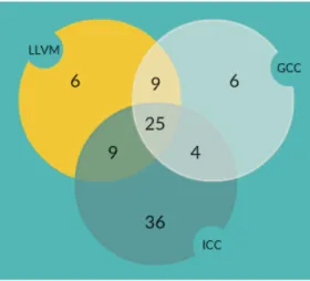
Figure 2.1: Number of loops vectorized by LLVM, GCC and Intel C Compiler in TSVC Benchmark We find that ICC performed better than GCC, which, in turn, performed better than LLVM for TSVC benchmark suite. Out of the total possible 151 loop kernels, 70 were vectorized by LLVM,

(15)

82 by GCC and 112 by the Intel C Compiler. We represent the results in a Venn diagram in Fig. 2.1.

Analysis: We see that 59 loop kernels are vectorized by all the three compilers. However, there are 31 loops which remain non-vectorized by any of them. For some of the loops, ICC is able to partially vectorize it. In fact, there are 30 loops that are vectorized by ICC only. LLVM performs the worst among the three. A possible reason can be that since LLVM is a relatively new compiler, all latest features are not integrated in it. Currently, a new vectorization procedure called VPlan (https://llvm.org/docs/Proposals/VectorizationPlan.html) is being developed which incorporates a new framework for vectorization in LLVM. The superior performance of ICC can be attributed to the fact that the underlying architecture on which the tests are run is an Intel system. The runtime results are obtained by running each test kernel 10 times and calculating their mean values.

The chief causes for failure to do vectorization are described below:

• Failure to detect trip-count (loops-with-multiple-exits).

• Unable to resolve dependences between statements.

• Complicated access patterns like non-uniform access or indirect access.

• Complex control-flow (switch-case structures, goto statements).

• Failure to do scalar expansion.

• Function calls from loop body.

• Cost-model marking vectorization inefficient.

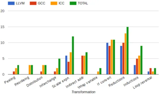
Figure 2.2: Comparison of LLVM, GCC and ICC with respect to the number of vectorized loops (Y-axis) v loop transformation type (X-axis) for TSVC benchmark

In Fig. 2.2 we see the number of loops vectorized by each compiler requiring a specific transfor-mation. The green bar represents the total number of loops for a specific type. As we can see ICC

(16)

gives the best performance. We also find that for several types, vectorization fails totally in case of LLVM. For the cases of loop distribution, wrap around variable detection and transformation, loop interchange, statement reordering and loop peeling, LLVM is not able to transform any of the loops. LLVM gives the best performance for If-convertible loops and scalar expansion. GCC is unable to reorder statements. Fig. 2.3 shows run times of both vectorized and non-vectorized loops in LLVM for TSVC. We find that for some cases the vectorized loops perform much better than the non-vectorized loops.

Figure 2.3: TSVC Runtime in seconds(Y-axis) of vectorized (blue cross) and non-vectorized (red dots) loop kernels of LLVM compiler. X-axis denotes loop number. Out of 70 vectorized loops, 19 had performance degradation with vectorization.

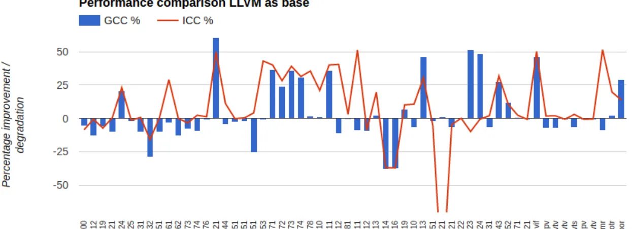
We also present a comparison of the run times of the loops successfully vectorized by all the compilers in Fig. 2.4. GCC and ICC running times are given by the red and yellow worms, while blue bar represents the LLVM run times. We find that for some cases, the vectorized run times are significantly different among the three compilers.

Figure 2.4: A comparison of run times of only those loops vectorized by all three compilers with LLVM as base line.

(17)

Analysis of MiBench and TORCH Benchmarks: Most of the loops extracted from MiBench and TORCH cannot be vectorized as they are real world programs and are not straightforward for vectorization. We carefully extracted the loops from C source files. We paid attention that loops with exactly similar structure and memory accesses patterns were not included more than once to avoid repetition. The chief hindrances to vectorization are dependences, function calls from the loop body, loops with multiple exits, loops with unknown trip count, and not being able to identify the loop control variable (specially in while loops). Fig. 2.5 describes the number of loop vectorized by the compilers for TSVC and MiBench kernels.

Figure 2.5: Comparison of number of vectorized loop kernels of TORCH and MiBench.

2.4 Conclusion

In this chapter, we show that the current major compilers do have specific areas in loop transfor-mation where they can be improved. Our analysis exposes these deficiencies in current generation compilers we studied, and provides direction for research in these areas. As far as we know, our work is the first study comparing the given compilers. As pointed out earlier, loop transformations need improvement in open source compilers. Also, transformations should be from the viewpoint of vectorization rather than being separate passes decoupled from vectorization. Another direction is to perform outer loop vectorization.

(18)

Chapter 3

A Short Study of Vectorization on

Tiled Code

3.1 Introduction to Tiling

Tiling [5] is a loop transformation which enhances data locality and thereby producing a better runtime. It partitions the iteration space of the loop into uniform tiles of given size and shape. Variation in size gives different results according the system cache size. The spape of the tile can be rectangular, hexagonal or diamond pattern among many others. Each have their share of benefits and disadvantages. By far, the most used pattern is the rectangular tiling.

Figure 3.1: A Tiling Example

The above example in Fig. 3.1 is taken from [6] describes how tiling is done. It represents a two-dimensional iteration space. The dots in the diagram represent the iteration points in the loop. The tile size can be varied as well as the shape. Loop tiling decomposes an n-dimensional loop nest into a 2n-dimensional loop nest where the outer n-dimensional loop nest iterate over the tiles and the inner n-dimensions iterate over a tile. In the above figure, the two dimensional loop nest is divided into 4 dimensions.

(19)

3.2 Description

This work tries to gauge the applicability and impact of vectorization on tiled code. Tiling is a coarse grain data locality optimizer. Vectorizer is a fine-grain optimizer. So, if we combine both of them we can produce optimal code. PluTo [7], a Practical and Fully Automatic Polyhedral Program Optimization System has been used to tile the loops. PluTo uses polyhedral analysis to find dependences in the loop nest. It forms an Integer Linear Program and finds the cost of transformation. Along with tiling, it can apply other loop transformations too. We use Polybench [8] to perform the study as it is a standard test suite for polyhedral compilation. After the tiled code is formed, it is then passed through LLVM vectorizer and the final code is generated. We compare the performance of the code with other given permutations below.

• Only LLVM without vectorization.

• LLVM with vectorization.

• Only PluTo with tiling and other wavefront transformations.

• LLVM and PluTo with tiling

• LLVM and PluTo with tiling and wavefront transformations.

3.3 Results

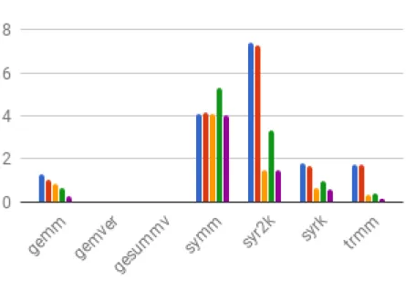
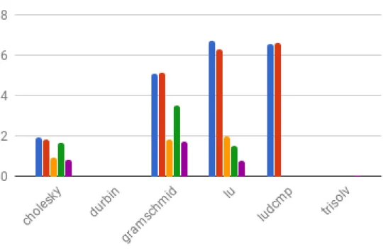
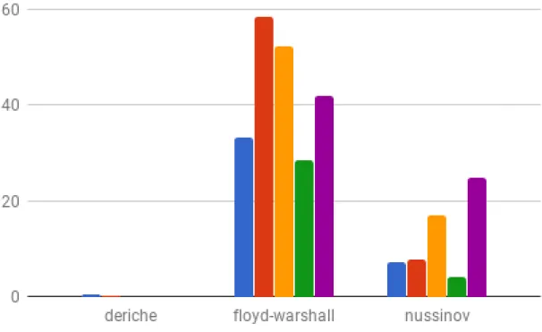
The results have been presented below. The blue bar represents 1, the red bar represents 2, yellow bar represents 3, green bar represents 4 and violet bar is represented by 5. In Fig. 3.3 Gemver and Gesummv are not visible because they have very small values compared to the others. In Fig. 3.4 Atax, Bicg and Bvt values are very less to be visible. In Fig. 3.5 Ludcmp values for 3,4 and 5 are not present because they are very very large and do not fit in the chart. This is the similar case for Deriche in Fig. 3.6. We find that tiled code is faster among all cases.

3.4 Analysis and Conclusion

We find that tiled code is significantly faster than non-tiled code. However, in a few cases (Deriche and Ludcmp) the time taken to execute is huge and does not fit into the diagram. The reason is the presence of a significantly large loop nest with high loop depth. In these cases, the tiled code increases the dimension of the loop depth even larger. So, during execution, due to limited size of the cache the data locality is worse than without tiling. Hence, the execution time becomes huge. Additionally, as expected, vectorization on tiled code improved the performance of the programs.

(20)

Figure 3.2: Performance Results on Datamining Benchmark set of Polybench

(21)

Figure 3.4: Performance Results on Kernel Benchmark set of linear-algebra in Polybench

(22)

Figure 3.6: Performance Results on Medley Benchmark set of Polybench

(23)

Chapter 4

Loop Nest Optimzation

4.1 Statement Reordering

4.1.1 Introduction

Statement reordering involves the process of ordering the statements inside a loop to break depen-dences and enable vectorization and other optimizations. We describe some introductory material before describing the algorithm.

4.1.2 Dependence Types Definitions

There is a memory dependence between two instructions if both access the same memory location at least one instruction is a write operation. If there is a dependence between two memory operations S1 and S2, we represent it as S1 S2, where S1 is executed before S2 and at least one is a write operation. The dependence can be read-after-write, write-after-read or write-after-write.

Loop Carried Dependence: A dependence is loop carried if the two memory operations occur in separate iterations of the loop. This type of dependences are also called inter-iteration dependence.

for (int i=1; i<N; i++){ S1: ... A[i-1] S2: A[i] = ... }

Loop Independent Dependence: A dependence is loop independent if both the operations on memory are performed in the same iteration of the loop. This type of dependences are also called intra iteration dependence.

for (int i=1; i<N; i++){ S1: ... = A[i] S2: A[i] = ... }

(24)

Lexically Forward Dependence: The dependence between two instructions or statements is lexically forward if the dependence follows the program order, ie. if there is a dependence from S1 to S2, then S1 comes before S2 in the program order as well as order of execution. A lexically forward dependence can be loop-independent as well as loop-carried. For example, in the below program, there is a RAW dependence from S1 to S2. Since the dependence follows occurs in the same iteration, it is loop independent.

Loop-carried Lexically forward dependence Loop Independent Lexically forward dependence for ( int i=0; i<N; i++) {

S1: A[i] = ... S2: ... = A[i-1] }

for ( int i=0; i<N; i++) { S1: A[i] = ... S2: ... = A[i] }

In the example below, there is a RAW dependence from S1 to S2. Since the dependence occurs between two iterations, it is loop-carried.

for (int i=0; i<N; i++) { S1: ... = A[i+1]

S2: A[i] = ... }

Lexically forward dependences do not inhibit vectorization as they follow the program order; only lexically backward dependences do.

Lexically Backward Dependence: The dependence between two instructions or statements is lexically backward if the dependence is against the program order, ie. If a dependence from S2 to S1 exists, then S1 comes before S2 in the program order. For example, the given program has a lexically backward dependence from S2 to S1. A lexically backward dependence is always loop-carried.

for (int i=1; i<N; i++){

S1: ... = A[i-1] S2: A[i] = ... }

A lexically backward dependence is generally bad for vectorization. If the dependence distance for such cases is greater than or equal to the Vectorization Factor, then vectorization can be per-formed. If not, we may have to reduce the Vectorization Factor, thereby decreasing the speedup. Our instruction reordering pass focuses on breaking this backward dependence by reordering the concerning instructions, thereby exposing vectorization. Any dependence which is lexically forward, regardless of its iteration distance, it will always be vectorizable.

4.1.3 Description

A Motivating Example: We explain the algorithm of the reordering method via a motivating example. We then describe the algorithm in detail. The following loop (s212) is taken from the TSVC benchmark suite.

for (int i = 0; i < LEN-1; i++) { S1: a[i] *= c[i];

S2: b[i] += a[i + 1] * d[i]; }

(25)

The LLVM IR pseudo code for the example can be written as: 1. I1: Load c[i]

2. I2: Load a[i] 3. I3: Mul1 = c[i]*a[i] 4. I4: Store Mul1 to a[i] 5. I5: a[i+1]

6. I6: Load d[i]

7. I7: Mul2 = a[i+1]*d[i] 8. I8: Load b[i]

9. I9: Add1 = b[i]+Mul2 10. I10: Store Add1 to b[i]

In the above loop, we see three memory dependences:

• WAR dependence between I2 and I4. This is lexically forward loop-independent dependence.

• WAR dependence from I5 and I4. This is lexically backward loop-carried dependence.

• WAR dependence from I8 and I10. This is lexically forward loop-independent dependence. Due to the presence of lexically backward dependence this loop is not vectorized by the loop vectorizer. Our instruction reordering pass aims to reorder the instructions in such a way that this loop becomes vectorizable.

We get the memory dependences from the LLVM infrastructure. We build the dependence graph from those dependences. Additionally, we also get the exact dependences from the polyhedral anal-ysis in Polly. The information provided by Polly is added to the dependence graph, if not already given by the conservative analysis of LLVM infrastructure. The dependence graph of the above program will be given by (I2→I4),(I5→I4),(I8→I10). We can see that in most cases the graph will be a forest with multiple directed components.

Building Instruction Level Memory Dependence Graph: The LLVM Intermediate Rep-resentation is a low-level repRep-resentation which is closer to assembly, but is expressive to be human-readable. All the transformation optimization passes of LLVM run on this intermediate represen-tation. The dependence analysis information which is provided by the LLVM Infrastructure is in terms of instructions in this IR (Intermediate Representation). So, the granularity of the dependence is instruction level. The LLVM infrastructure provides all memory dependence information among load/store instructions in the LLVM IR. However, the dependence information provided by LLVM is conservative in nature.

As the analysis by LLVM is conservative, we also get the exact dependences among instructions from Polly-as-an-Analysis pass which we developed. The dependence information given from LLVM is combined with Polly to form the dependence graph on which we base our transformation.

(26)

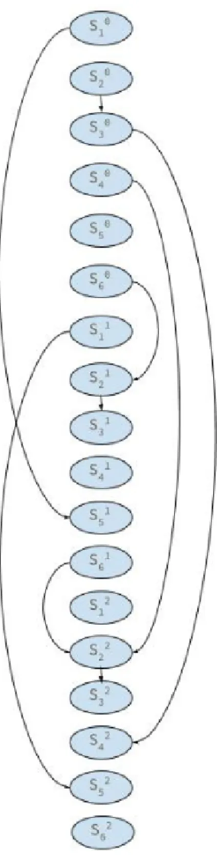
Load/Store Reordering: Reordering of instructions in LLVM IR within an innermost loop may expose vectorization. Before explaining reordering, we need to explain some types of dependences. We now perform a simple topological sort of the dependence graph. This needs to be done to each acyclic directed component to get an ordering of the instructions. However, we need to perform the sort in the program order of the instructions. For our example, we first start with I2→I4, then, I5→I4 and then I8→I10. Doing this in order preserve the program order of the instructions in the LLVM IR. The topologically sorted instructions will be given by I2→I4→I5→I4→I8→I10. We now delete any repeated instructions keeping the last instance of the instruction in the sorted list. So, the first occurrence of I4 is deleted to get the final sequence as I2→I5→I4→I8→I10. The final sequence of instructions follows the dependence order as well as the program order.

We now populate the rest of the IR instructions by following the use-def chain information and building the dependent instructions from bottom-up. It may happen while building up the instructions that a cyclic dependence is formed which clashes with the dependence order in the memory dependence graph. In those scenarios, we bail out. It is explained in Fig. 4.1.

Figure 4.1: Building the sequence of Instructions via the use-def chains

Now we have a sequence of instructions which needs to be inserted in the basic block of a loop. For the above example, the reordered instructions are given below. As we can see, the instruction I5 has come above I4, thereby breaking the dependence. If we analyze the loop, the change that we did is loading a[i+1] in I5 above storing to a[i] in I4. This does not impact the semantics of the loop but exposes vectorization. The LLVM vectorizer is now able to successfully vectorize the loop after this transformation.

1. I1: Load c[i] 2. I2: Load a[i] 3. I5: Load a[i+1] 4. Mul1 = c[i]*a[i] 5. Store Mul1 to a[i] 6. I6: Load d[i]

7. I7: Mul2 = a[i+1]*d[i] 8. I8: Load b[i]

(27)

9. I9: Add1 = b[i]+Mul2 10. I10: Store Add1 to b[i]

We present the steps to be done below:

1. Get the memory dependences present in an innermost loop from LLVM infrastructure. 2. Get the memory dependences from Polly via Polly-as-a-Pass interface.

3. Construct the memory dependence graph from those dependences. 4. Check for backward dependences. If no such dependence present, we exit.

5. Perform a topological sort of all the directed components of the dependence graph to get a sequence of instructions.

6. Delete all repeated instructions in the sequence except the lowest occurrence of that instruction in the list.

7. For each basic block in the loop

• Get a subset sequence of the instruction which belong to that basic block. We do not reorder instructions between basic blocks.

• Build up the rest of the dependent instructions via use-def information to get a complete sequence of instructions. If we find the presence of cycle, we exit.

• Replace the instructions of the basic block with this new sequence of instructions.

4.1.4 Results and Conclusion

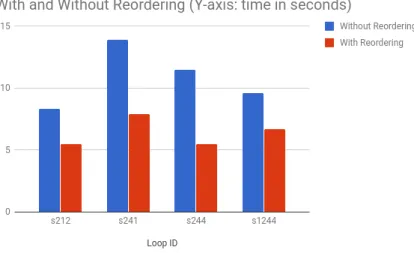
Architecture: We perform our analysis using an Intel(R) Xeon(R) CPU E5-2690 v4 @ 2.60GHz processor. It has maximum of 56 Threads with cache size of 35MB. The RAM size is 32GB. We find that four loops out of 151 loops where able to achieve a 40% speedup after reordering. Fig. 4.2 describes the performance in TSVC. As a future work, control flow in loops needs to be handled.

4.2 Improving Loop Parallelism with unrolling and explicitly

parallel constructs

4.2.1 Introduction

In the previous section, we tried to expose vectorization by reordering the statements so that back-ward dependences are transformed to forback-ward whenever possible. We try to extend this work to optimize loop in which vectorization is not possible even by reordering. In this case, we reorder the statements in a loop to expose maximum parallelism.

(28)

Figure 4.2: Speedup achieved in TSVC

4.2.2 Related Work

Chen et. al [9] reordered the loop statements to expose maximum parallelism for DO-ACROSS loops. The statements in the loop are reordered to decrease the delay between each loop iteration. However, since this work is before the era of vectorization, it does not consider vectorization and hence opportunities are missed. Liu et. al [10] used retiming to transfer the dependence edge weight of other nodes to maximize the non-zero edge weight in the dependence graph. However, this particular optimization solely targeted vectorization. So, if a loop is not vectorizable even after retiming, parallelism opportunities are lost. Jensen et. al [11] targets explicitly parallel directives present in programs. It adds the dependence information from the directives into the dependence graph. This opens opportunities for vectorization. However, this depends on user-supplied information. Chatarashi et. al [12] does the same dependence analysis but used polyhedral analysis to form the dependence graph.

4.2.3 Description

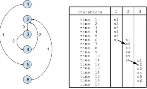
We present our method via a motivating example. We take the same example given in [9] as described by Fig. 4.3. As we can see, due the presence of dependence S6→S2, the overlapping of statements to be executed in parallel is restricted. This forces serial execution of the code.

We define S(i,k) as the time stamp of execution of statement S(i) where i is the statement sequence in the original order of the loop. k is the iteration number for the loop during execution. So for a statement S(i) at iteration number 1, the time stamp will be S(i,1). Similarly, for iteration 2 it will be S(i,2), and so on and so forth. The loop is unrolled to an unroll factor of the maximum dependence distance. Hence, we get 0 ≤ k and k ≤ {maximum dependence distance} and 1 ≤ i ≤ {no. of statements in loop}. The maximum dependence distance is the maximum of all the dependence distances present in the dependence graph.

For the given example in Fig. 4.4, we get the following constraints. Since the maximum depen-dence distance is 2, k ranges from 0 to 2. So, the loop is unroll thrice and then the constraints are formed. For the dependence between S1→S5, the constraint will be S(1,0) + 1≤S(5,1) [ie. S(1) at

(29)

Figure 4.3: A Motivating Example and the corresponding dependence graph. We see the constraints in overlapped execution due to the dependence from S6→S2

0th iteration should precede S(5) at 1st iteration]. Similarly, S(1,1)+1≤S(5,2) [S(1) at 1st iteration should precede S(5) at 2nd iteration]. We can write the remaining constraints as: S(1,0) + 1 ≤ S(5,1) , S(1,1)+1 ≤S(5,2), S(2,0)+1 ≤S(3,0), S(2,1)+1≤S(3,1), S(2,2)+1 ≤S(3,2), S(3,0)+1≤ S(4,2), S(4,0)+1≤S(2,2), S(6,0)+1≤S(2,1) ,S(6,1)+1≤S(2,2).

We need to get the minimum possible timestamp of each statement. So, we make the objective function such that the sum of all the timestamps is minimum. So, the objective function for the set of constraints is given by Minimize{sum(S10,S20,...,S60, S11,S21,...S62)}. The solution of the Integer Linear Program (ILP) will give the timestamps of each statement. Solving for the Integer Linear Program we get {S(1,0), S(2,0),S(4,0), S(6,0), S(1,1), S(4,1), S(6,1), S(1,2), S(6,2)} with timestamp 0, {S(3,0), S(2,1), S(5,1), S(2,2), S(5,2)} as timestamp 1 and {S(3,1), S(3,2) ,S(4,2)} with timestamp 2. The extended dependence graph is presented in Fig. 4.5. The source code in Fig. 4.4 is transformed to Fig. 4.6.

So, in general terms, given a loop L with given constraints:

• Set of statements S(i), where ‘i’ is the sequence number of the statement.

• Set of dependence distances D, where Dij represents the dependence distance between S(i) and S(j)

We summarize the solution as follows:

• Form the dependence graph for the loop L.

(30)

Figure 4.4: Motivating Example Source Code

• Define and solve the ILP to get a timestamp ordering for each statement in the unrolled loop.

• Segregate the statements into different collections.

• Add OMP parallel directive to each collection to parallelize it.

4.2.4 Conclusion

The above method depends heavily on the amount of parallelism present in a loop nest. Also, the incorporation of resource constraints in the ILP can enhance the accuracy. Additionally, a cost model can be prepared which judges the cost of the transformed code against the original code before transformation.

4.3 A Dynamic Programming Approach to Loop

Distribu-tion

4.3.1 Introduction

Loop Distribution is a popular and well-known compiler optimization where a single loop is divided into multiple loops over an exhaustive set of statements in the original loop. All the loops iterate over the same index range. This transformation can expose vectorization and thread-level parallelism. The chief task of this transformation is identifying the set of statements which will be contained in a distributed loop. We present a dynamic programming approach to find these sets.

4.3.2 Description

Dynamic programming is a computer programming method which was developed by Richard Bell-man. It simplifies a complicated problem by breaking it down into simpler sub-problems in a recursive manner. We follow the given procedure:

1. Build the dependence graph for the loop. The nodes of the graph denotes the statements and the edges denote the dependence between them.

(31)

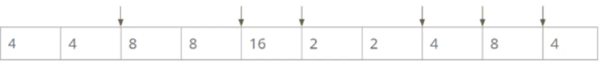
3. Assign Vectorization Factor to each component. Vectorization Factor is the maximum number of elements that can be loaded in a vector register. The factor depends on the data type of the element.

4. Topologically sort the SCCs to arrive at a sequential ordering of the SCCs.

5. Apply the dynamic programming based approach on the sequential ordering to get a packing. Apply this to all the possible sequential orderings. The approach is described later.

6. Find the minimum packing cost ordering and distribute the loop according to that packing order.

The approach we follow draws idea out of a famous dynamic programming problem: Rod Cutting Problem. If we are given a rod of length ‘n’ and the selling price of all pieces of the rod possible of all length less than equal to n, we need to find the ideal cutting of the rod so that we derive the maximum value after selling the pieces. As with other dynamic programming problems, this too follows the optimal substructure and overlapping subproblems criteria. However, our problem has two key differences than the standard rod-cutting problem:

• Each cut value is different for the same size cut due to variation in the Vectorization Factor.

• We cut only at those positions where the Vectorization Factor changes. This is an optimization measure since the performance of n lines code with Vectorization Factor K is always better than the performance of n1 and n2 lines of code, where n1+n2=n with the same vectorization factor.

The Fig. 4.7 shows a sequence of SCCs found after a topological sort with a Vectorization Factor for each of them. Our task is to find the distribution boundaries in the sequence.

We present the algorithm in Fig. 4.8. The notations are described below.

• SCClist : List of SCCs.

• VF[i] : Vectorization Factor of SCC i.

• N : total number of SCCs.

• p[i,j] : Cost of packing of SCCs of length (i,j), where i is the index from where we start the cut and j is where we stop. So the SCCs between i,j stays in a single loop. This information is calculated as and when required in O(1) time.

It is a recursive algorithm that identifies the positions where the distribution boundaries need to be made. It closely follows the rod-cutting algorithm. Line[1-2] denotes that when the length of the list is zero we return. In Line 4 we make ‘i’ as the base of the distribution boundary and attempt to make a cut after this boundary. We start the iteration for each possible SCClist boundary in line 5. We initialize the ‘q’ as∞. Until we reach the end of the SCClist or if the Vectorization Factor does not change, we proceed for the next possible distribution boundary in line 6. The recurrence relation is defined in line 7. We make the distribution boundary at ‘j’ and proceed to find the cost for the other cut of the SCClist in a recursive call. Finally, we return the minimum cost.

(32)

(33)

Figure 4.6: Modified Version of the source code following the transformation.

(34)

(35)

Chapter 5

Interprocedural Register

Allocation in LLVM for

ARM32/AArch64

5.1 Introduction

Register Allocation deals with the hard problem of assigning a very few registers among a large set of program variables. Generally, register allocation takes place for each procedure separately in standard register allocation algorithms. Register Allocation is described in the Fig. 5.1 For LLVM. We see that before the generation of machine registers, Register Allocation takes place. However, sometimes various optimization opportunities are missed due to not using the additional information of allocating a set of registers for the register allocation of another procedure. Interprocedural Register Allocation deals with this idea and tries to exploit this information. It uses the information of allocated registers in another procedure to allocate registers in its own. The architecture is presented in Fig. 5.2

Figure 5.1: Register Allocation in LLVM

Various contemporary work has been done on the idea of Interprocedural Register Allocation. Chow [13] and [14] first use the idea of Interprocedual Register Allocation. It constructs the call graph and proceeds with depth-first ordering of the callgraph. A callgraph represents the calling relationship among procedures. Nodes in the callgraph represent a procedure. A directed edge

(36)

Figure 5.2: Interprocedural Register Allocation in LLVM

from Node A to B in the callgraph represents that A calls B. The papers use the idea of caller-saved registers. In general, a set of registers in the CPU are designated by hardware as callee-caller-saved registers. The values in these registers should be preserved across a procedure call. This contract is described in the Calling Convention(CC) for the specific target. If the values are to be overwritten by a procedure, those values must be spilled before overwriting and then must be restored by that procedure. Since the callee procedure is responsible for saving/restoring the values of these registers, they are called callee-saved registers. The cited paper tries to replace uses of callee-saved registers by caller-saved registers. This work deals with implementation of Interproceural Register Allocation on LLVM compiler.

5.2 Description

We describe our work with examples and differentiation with normal register allocation. Let us have a demo architecture with 16 registers R0-R15. Out of these registers, let R4-R8 be the callee-saved registers. We will take a look how normal register allocation works in Table 5.1 and then compare it with Interprocedural Register Allocation in Table 5.2. We see that registers R9 and R10 are not used by the callee procedure. This information is available to the caller. Hence, the caller can now skip spilling the contents of R9 and R10 across the call site thereby saving precious memory access time.

Table 5.1: Standard Register Allocation Example 1

Caller Callee

Uses R0-R10 registers Uses R0 - R5 registers.

R4-R8 are callee-saved, the caller need not save them. R9 and R10 should be saved by caller.

R9, R10 registers are spilled/restored if live across the call site.

We also see another advantage of IPRA in the example below. In standard register allocation a set of registers are declared as callee-saved registers. In IPRA, we introduce caller-saved registers in place of callee-saved registers. In Table 5.3 we see that the callee spills/restores R4-R8 registers as they are callee saved. However,the caller only uses registers R0-R2. So, instead of callee spilling/restoring 5 registers, the caller can spill/restore 3 registers thereby saving the cost of 2 extra registers. This

(37)

Table 5.2: Interprocedural Register Allocation Example 1

Caller Callee

Uses R0-R10 registers Uses R0 - R5 registers.

R4-R8 are callee-saved, the caller need not save them. R9, R10 not used by callee.

R9, R10 registers are not spilled/restored across the call site.

can be seen in Table 5.4.

Table 5.3: Standard Register Allocation Example 2

Caller Callee

Uses R0-R2 registers Uses R0-R10 registers.

Spills/Restores R4-R8 registers which are callee-saved

Table 5.4: Interprocedural Register Allocation Example 2

Caller Callee

Uses R0-R2 registers Uses R0-R10 registers.

Spills restores R0-R2 registers which are caller-saved

Due to IPRA caller does not use the registers which have been changed by the callee and this saves some spills/restores. However, if the callee procedure be big enough to use most registers and thus there may not be enough registers available for the caller to pick from and thus use the same registers as used by the callee. In IPRA, if the same set of registers are used by the caller/callee, it is the responsibility of the caller to preserve the register values across callsite. So, we do not reset register bit as per calling convention and remove the standard callee saved registers from the register mask. Since IPRA depends on the target architecture, target specific things are to be handled by it. IPRA was implemented in LLVM for x86 platform. This work deals with making IPRA work for AArch64 and ARM32 platforms. We need to understand how IPRA is implemented in LLVM. However, this optimization is applied to select cases. This optimization is applied only on function calls with following properties: internal linkage, not recursive, no indirect call and should not be optimized as tail call. This is because for the functions which are recursive or indirectly called or tail call optimized, we cannot set the standard callee saved registers as null because those registers will behave in their own way of following the calling convention. The general thumb rule is this: If the caller is following the IPRA convention, the callee should follow the same. In such situations parameters and return value can not be passed correctly or registers can become corrupted since IPRA optimization breaks normal calling convention. Due this we only apply this optimization to functions which have internal linkage and hence are in the same compilation unit.

IPRA in LLVM consists of a sequence of four passes in LLVM which are described as follows:

• DummyCGSCC pass: This pass is a CallGraphSCC pass in LLVM which means that the pass works on the callgraph. Since, the IPRA algorithm works on the callgraph in a bottom up fashion, the pass alters the code generation order of the callgraph procedure from bottom up so that the register information of a child procedure is known to the parent procedure before its register allocation.

(38)

• PhysicalRegisterUsageInfo pass: This pass is an immutable pass and does not do any transformation. It holds a map data structure which stores the registers used by a particular procedure. It also makes available interface to insert data in the map.

• RegUsageInfoCollector pass: This is a machinefunction pass and runs after register al-location has been performed on a procedure. It collects the registers which are used by the procedure and stores in the map which are accessed by the PhysicalRegisterUsage pass inter-face.

• RegUsageInfoPropagate pass: It is also a machinefunction pass but runs before register allocation. At every callsite, a register mask is formed for that particular call which store the registers which will be preserved across the callsite. This pass understands the registers which are not used by the callee procedure and appends those to the register mask.

In the following sections, we describe the various issues and workarounds done to make IPRA compatible on AArch64/ARM32 platforms.

5.2.1 Invalid Return Address

In ARM32, following the call to a procedure, the register LR(Link Register) stores the return address of the caller. After the execution of the callee, the control returns to the caller and the return address must be loaded from the LR register. Due to this reason, LR is treated as a callee-saved register in the calling convention. However, IPRA does not follow normal calling convention. So, LR is overwritten in the callee without saving and when the control tries to jump towards the location pointed by the LR register, we get a segmentation fault since the LR is corrupted. So, we ensure that the CC is followed for this particular register. The situation is illustrated in Fig. 5.3. This situation is also formed for the Stack Pointer(SP) register for AArch64.

5.2.2 Weak Symbol in separate Compilation units

A weak symbol is a specially annotated symbol during the linking of Executable and Linkable Format (ELF) object files. By default, a symbol in an object file is a strong symbol. During linking, a strong symbol can override a weak symbol of the same name. If there are multiple strong symbol, compiler generates an error during linking phase. However, if multiple weak symbols are present during linking, the compiler picks any one of them. This error is formed due to this reason. When two compilation units are compiled separately having weak symbols with similar name, the standard calling convention ensures the use of registers. But since it is not followed in IPRA, a procedure in module A may call another another similar named procedure in Module B (Fig 5.4). Since, register allocation of routineA is done according to the register use of ‘bar’ in its module, when the compiler picks the ‘bar’ version from Module B, it generates an error. The scenario is described in Fig. 5.5.We solve this error by ensuring that the normal calling convention is followed whenever a call is made to a function with weak linkage.

5.2.3 Error due to Fast Calling Convention

Fastcc calling convention is described in the LLVM Language Reference Manual [15] as follows: “Fastcc calling convention attempts to make calls as fast as possible (e.g. by passing things in

(39)

Figure 5.3: Invalid Return Address in the LR register

registers). This calling convention allows the target to use whatever tricks it wants to produce fast code for the target, without having to conform to an externally specified ABI (Application Binary Interface). Tail calls can only be optimized when this, the GHC or the HiPE convention is used. This calling convention does not support varargs and requires the prototype of all callees to exactly match the prototype of the function definition.” When a call is made following the fastcc convention, we do not remove the callee-saved registers from the Register mask to ensure that the responsibility of the saving/restoring the registers is on the callee and not on the caller. The scenario is described in the following Fig. 5.6.

5.2.4 Error in Tail Call Instruction

In ARM32 there is an instruction TCRETURNdi which is generates when a tail call is made to a procedure. However, this instruction does not have a register mask to denote those registers whose states have been consistent across the callsite. In a situation where, lets say procedure A calls B, and B tailcalls C; such that the tailcall instruction in B is a TCRETURNdi instruction. Since the instruction does not contain a register mask, the used registers of procedure C are not propagated to procedure A, thus breaking the IPRA propagation of register information from child to parent procedure. The calling procedure A does not know about C and uses registers which are modified by C as caller-saved convention is followed. This results in corrupt registers.

This problem can be solved by two ways. One way is checking for the generation of this particular instruction and not following IPRA. Another way is to generate Register Mask even if this instruction is generated by the ARM32 backend. We follow the second approach.

(40)

Figure 5.4: Weak Symbol in separate Compilation units

5.3 Results

The following figures explain the results of IPRA. We analyze the results in different aspects:

• The Performance impact of IPRA

• The Code Size impact of IPRA

We analyze the results on both ARM32 and AArch64 platforms. The baseline and the run columns represent a score given by a scoring mechanism. The higher the score the better is the result of IPRA for performance. For code size, lower is better. When we get a better run score than the baseline we can say that the code size has reduced or the performance has improved significantly. Green color in Difference column represents a markedly better performance or code size reduction. Red color represents downgrade in performance or increase in code size after IPRA. When the Dif-ference is colored yellow, we may infer that there has been very minimal change in performance or code size to warrant an improvement or degradation.

Performance in AArch64We find that for SPEC benchmark,libquantum performs exceedingly well with a difference score of 27. The rest of the cases have very small improvements or degrada-tions. For Non-spec benchmarks likeAndroid library, eembc, openssl and linpack, there are no major improvement of degradation. In code size, the most benchmark show a reduction in code size which is expected due to elimination of many spills/restores.

Performance in AArch64For AArch64,libquantum performs worse than standard register allo-cation. However, we get improvement formcf andsoplex for SPEC 2006 benchmark. We get code size reduction foreembc benchmark.

(41)

Figure 5.5: Executable Level View of Weak Symbol in separate Compilation units

5.4 Conclusion and Future Work

Interprocedural Register Allocation is an useful technique which can enhance the runtime of pro-grams. However, IPRA may or may not be useful in all cases. We need to develop a cost model to compare IPRA vis-a-vis normal calling convention and take the path which gives better results. We can do this by getting the number of spills/restores for each approach and then deciding to generate code. Also, since Register Allocation depends heavily on the underlying architecture, the target information can be included in the cost model.

(42)

Figure 5.6: Error due to Fast Calling Convention

Figure 5.7: Error in Tail Call Instruction. A Pseudo instruction TCRETURN is generated without a register mask

(43)

Chapter 6

VoPiL: Verification of OpenMP

programs in LLVM

6.1 Introduction

High Performance Computing(HPC) is a vital part of computing which is growing in importance rapidly. In the recent years, a significant amount of work has been put in increasing the scope of HPC. Additionally, a huge amount of increase in the computing power has been seen in recent times. OpenMP is a directive based API which enables the programmer to incorporate various directives in the source-code to exploit the parallel sections. However, incorporating directives is a difficult task for the programmer as various dependences need to be preserved in order to generate correct code. Various analysis tools have been developed over the years to verify user supplied OpenMP directives. They can be classified into two- static and dynamic. VoPiL is a static analysis tool build over the LLVM source code. LLVM is a popular compiler which is modular in nature. It supports various programming languages like C, C++ and Fortran. All the analysis and transformations are applied on the Intermediate Representation in LLVM.

We describe a static verification tool for OpenMP constructs in LLVM. This tool is built on top of LLVM source code and works on the Intermediate Representation(IR) of LLVM. As a result, it supports verification of OpenMP constructs on all the source languages that LLVM supports. Currently, it supports verification of data races in an important class of common OpenMP constructs. We use the polyhedral model built into LLVM called Polly as well as native dependence analysis of LLVM for detecting race conditions. We are able to detect very subtle race conditions which are not apparent to even expert programmers. We illustrate the efficacy of our tool by a set of various motivating examples as well as widely used benchmarks. Finally, we also apply our tool to select open source softwares with OpenMP constructs.

6.2 Related Work

Datarace detection in parallel programs have been a highly studied problem in the literature. There are various methods and tools available to detect data races in parallel programs. With the

(44)

ad-vent of OpenMP, this task was extended to verify data races in explicitly parallel programs. In general, there are two ways of detection of user-supplied OpenMP pragmas: static and dynamic. Some tools combine both static and dynamic techniques. Each one of them has advantages and disadvantages. Dynamic detection involves instrumentation of the code and try to find data races by actually running the code. Static detection [16], [16] is done by analyzing the code and statically detect data races without running the code. This is a great advantage. ARCHER [17] uses static analysis (polyhedral dependence analyzer) to detect sensitive regions and then runs TSan [18] on them to detect races.

Polyhedral Analysis and transformation is a mathematical modeling of program regions following which transformation are performed on those regions. For this, the program in represented in a different model and the transformed code is re-generated from the model after the transformation. Basupalli et. al [19] uses polyhedral analysis to analyze OpenMP directives in a loop and suggest errors/warnings for the programmer. This was incorporated as a plugin in Eclipse IDE using Alp-haZ [20] language for the analysis and transformation. Our work draws inspiration from this paper. We not only implement a similar functionality in LLVM, which has a greater impact due to the LLVM IR, but also extend the analysis to detect even more race conditions.

6.3 Description

We first find out the particular directives which are very frequent in the popular benchmarks and those directives which have a greater occurrence frequency. We analyze popular OpenMP bench-marks like NAS Parallel [21], Rodinia [22] and SPEC OMP 2012 [23] benchbench-marks. Fig. 6.1, Fig. 6.2 and Fig. 6.3 gives the frequencies of occurrences of various OpenMP directives in NAS Parallel, Rodinia and SPEC OMP 2012 benchmarks.

Our tool is developed on the top of LLVM compiler v6.0. The architecture of our tool is described in Fig. 6.4. It is developed over the Intermediate Representation of LLVM as an analysis pass. It uses Polly, the Polyhedral Optimization tool implemented for LLVM, for getting information about parallelism present in the program. However, the scope of detection of Polly is only limited to affine programs. To increase the scope, our pass also uses the dependence analysis present in the LLVM infrastructure. The toolchain is divided into three major parts:

• Detection of explicitly parallel constructs in LLVM IR.

• Analysis for detection of race conditions.

• Display of proper diagnostic messages.

6.3.1 Detection of explicitly parallel constructs in LLVM IR

OpenMP explicitly parallel constructs are added by the source code programmer in the source lan-guage. The directives start with #pragma and clauses are added following the directive. Detecting the directives in the source language is easy as we have to match the directive names and then ana-lyze the section marked by the directive. However in LLVM this becomes tricky as we detect these directives in the Intermediate Representation (IR). The C/C++ front end of LLVM clang outlines the directive section into a separate function. It inserts various OpenMP library function calls in IR.

(45)

Figure 6.1: Occurrence Frequency for OpenMP directives in NAS Parallel benchmark.

Every directive and their corresponding clauses have a specific pattern in the IR. We match those patterns and identify the directives along with the sections where they apply.

6.3.2 Analysis for detection of race conditions

Following the identification of the directives, we analyze the regions to find race conditions. For de-pendence analysis we rely on the Polly, the Polyhedral Optimizer in LLVM, as well as the dede-pendence analysis from LLVM Infrastructure. We do this because of Polly is limited to affine control loops only while LLVM dependence analysis has a broader scope. However, Polly is more precise in detecting dependences. We incorporate the race conditions detected by [19]. The race conditions detected are:

1. Detection of dependence violation by parallel loopsThis detects if a loop which has been marked as parallel explicitly have some dependence between the loop iterations. It employs Polyhedral Analysis of Polly, the Polyhedral Optimizer of LLVM. This is the most important criteria that needs to be analyzed for detection of race conditions.

2. Write Conflict With Shared VariablesThis checks that when multiple statements write into the same memory location, these statements cannot be executed at the same time instance, ie. in parallel. An example taken from [19] is shown below.

(46)

Figure 6.2: Occurrence Frequency for OpenMP directives in Rodinia benchmark.

#pragma omp parallel for private(j) for (i = 0; i < N; i++)

for (j = 0; j < i; j++) { S1 : A[j] = a[i,j]; S2 : B[i,j] = A[j]; }

We see the loop is declared parallel on the outer dimension. However, different threads, with different values of ‘i’, may access A[j] when ‘j’ is similar. So, there exists a potential race condition. We use the techniques described in the paper. We also extend the work with additional checks. We check for dependences between iterations in loop marked with #pragma omp simd.

3. Verify Master and Single directiveWe detect race conditions on master directives as given in the code below. ‘Scalar’ is declared as a shared variable in the parallel section. There is a ‘master’ directive inside this section. The variable scalar is read in the parallel section and written inside the master section. There exists two data races in this section: between S1,S2 and S2,S3. If master is replaced by a single directive, there will be a data race between S1,S2. The race between S2,S2 will not happen as there is an implicit barrier at the end of the master section. This race can also occur in critical section.

(47)

Figure 6.3: Occurrence Frequency for OpenMP directives in SPEC OMP 2012 benchmark. #pragma omp parallel shared(scalar) {

...

S1: ... = scalar //Read ...

#pragma omp master/shared {

S2: scalar = ...; //Write } ... S3: ... = scalar; //Read ... }

4. Verification of Private, Shared and Reduction ClausesWe now describe verification of private, shared and reduction clauses for parallel for directives. When a variable is declared as private, separate copies of the variable are made for each of the threads. If the variable is declared as shared, it can be simultaneously accessed by each of the thread as there are no copies. When a variable is declared as reduction, the variable should have private copies for each thread. However, during update the private copy of a thread is written to the global copy atomically so that no other thread updates it in parallel; thereby avoiding a potential race. We verify a reduction variable by these properties.

Each thread has a copy of a variable that is declared private. So, when a variable is updated and not declared private, a race condition will occur. Hence, variables that are written to should be declared as private. Similarly, variables which are only read can be declared as shared. Reduction variables are also written to. In the below example, variable j should be

(48)

Figure 6.4: Architecture of OpenMP construct verification in LLVM

declared as private.

#pragma omp parallel for for (i=0;i<100;i++)

for (j=0;j<100;j++) a[i][j]=a[i][j]+1;

6.3.3 Display of proper diagnostic messages

Our third task is to display user-understandable diagnostic messages when the program in verified. This is very important as ambiguous or imprecise reporting will make the entire effort of detection and analysis lose importance. For getting the diagnostic messages, the program needs to be compiled with-gflag in LLVM. This ensures that source-level debugging is enabled and the debug information is present in the LLVM Intermediate Representation. During the analysis, we maintain a map where the instructions in the IR is mapped to the source variables. Hence, we are able to emit diagnostic messages like line number of the loop,and the particular source variable which causes data race.

6.4 Results

We run our analysis on Dataracebench [24], a benchmark suite for systematic evaluation of data race detection tools. It was developed by Lawrence Livermore National Laboratory (LLNL) and published in 2017. It contains two sets of benchmarks: one set consists of microbenchmarks with

(49)

known data races, the other set consists of microbenchmarks without any known data races. The set of microbenchmarks with known data races helps us evaluate the True Positives(TP) and False Negatives(FN) of the benchmark. Similarly. the other set without known data races gives us the true negatives(TN) and the false positives(FP). We briefly describe these criteria for a benchmarking tool.

• True Positive (TP):If the evaluation tool correctly detects a data race present in the kernel it is a True Positive test result. A high number of true positives represents a better tool.

• True Negative (TN): If the microbenchmark does not contain a known race and the tool does not detect any race falsely, then it is a true negative case. A high number of true negatives represents a better tool.

• False Positives (FP):If the microbenchmark does not contain any race, but the tool reports a race condition, it a false positive. False Positives should be as low as possible. Generally, static race detection tools have a greater rate of false positives than dynamic race detection tools.

• False Negatives (FN):False Negative test result is obtained when the tool fails to detect a known race in the microbenchmark. These are the cases that are missed by the tool. A lower number of false negatives are desirable.

The results of our tool in Dataracebench v1.2 is described as follows. We divide the results in 4 separate tables: Table 6.1 and Table 6.2 gives the performance on microbenchmarks with known data race. Table 6.3 and Table 6.4 gives the performance results in microbenchmarks without known data races. Column 1 denotes the microbenchmark name, Column 2 gives a short description of the benchmark and Column 3 specifies whether our tool detects data race for the corresponding microbenchmark. The columns marked ‘NP’ are those which are OpenMP v4.5 and not supported in LLVM6.0 on which our analysis was built. The columns marked ‘N*’ are those for which the detection could not be done. Those are, hence, considered as failed cases.

We find that in the microbenchmarks with known data races, 33 out of possible 60 data races were successfully detected. In the set of microbenchmarks without known dataraces, 33 out of pos-sible 57 microbenchmarks were accurately detected as race free.

We compare the results of our static analyzer with other analysis tools like Helgrind, Thread-Sanitizer, Archer and Intel Inspector for Dataracebench v1.0. These are dynamic analysis tools, ie. they instrument the code and run them to find out potential data races. Out tool does static analysis and hence does not require to be run. This gives this tool an advantage. However, out tool needs to be compared with other static analysis tools to get a complete picture of the efficacy of our tool. In Fig. 6.5 we get the comparison between our tool and other mentioned tools. We find two columns marks as ‘Race:Yes’ and ‘Race:No’. The former represent the microbenchmarks with known data race, the latter the ones without. We also see two columns marked ‘TP/FN’ and ‘TN/FP’. Values in this columns denote those cases which yielded both presence and absence of race on multiple runs. Thus, these columns are mentioned to include this ambiguity. The numbers of the tools except VoPiL are obtained from [24].

(50)

Figure 6.5: Comparison of race detection tools.

• Precision TP/(TP+FP): Precision the confidence that a case detect to be datarace is actually is. Thus a higher value of precision represents that the tool will more often than not identify a race condition when it exists.

• Recall TP/(TP+FN): Recall gives the total number of cases detect out of the maximum data races present. A higher recall value means that there are less chances that a data race is missed by the tool.

• Accuracy (TP+TN)/(TP+FP+TN+FN):Accuracy gives the chances of correct reports out of all the reports, as the name suggests. A higher value of accuracy is always desired and gives overall measure of the efficacy of the tool. Fig.6.6 gives the comparison of our tool with others on the basis of these metrics.

Figure 6.6: Comparison in metrics between the race detection tools.

6.4.1 Conclusion and Future Work

We described our tool VoPiL and compared with other analysis tools. We find the results very encouraging. Since our toolchain is build on top of LLVM, it supports all languages which are

Optimizations In Compiler: Vectorization, Reordering, Register Allocation And Verification Of Explicitly Parallel Programs