Direct Speech Reconstruction from Articulatory Sensor Data by Machine Learning

(1)

Direct Speech Reconstruction from Articulatory

Sensor Data by Machine Learning

Jose A. Gonzalez, Lam A. Cheah, Angel M. Gomez, Phil D. Green, James M. Gilbert,

Stephen R. Ell, Roger K. Moore, and Ed Holdsworth

Abstract—This paper describes a technique which generates speech acoustics from articulator movements. Our motivation is to help people who can no longer speak following laryngectomy, a procedure which is carried out tens of thousands of times per year in the Western world. Our method for sensing articulator movement, Permanent Magnetic Articulography, relies on small, unobtrusive magnets attached to the lips and tongue. Changes in magnetic field caused by magnet movements are sensed and form the input to a process which is trained to estimate speech acoustics. In the experiments reported here this ‘Direct Synthesis’ technique is developed for normal speakers, with glued-on magnets, allowing us to train with parallel sensor and acoustic data. We describe three machine learning techniques for this task, based on Gaussian Mixture Models (GMMs), Deep Neural Networks (DNNs) and Recurrent Neural Networks (RNNs). We evaluate our techniques with objective acoustic distortion measures and subjective listening tests over spoken sentences read from novels (the CMU Arctic corpus). Our results show that the best performing technique is a bidirectional RNN (BiRNN), which employs both past and future contexts to predict the acoustics from the sensor data. BiRNNs are not suitable for synthesis in real-time but fixed-lag RNNs give similar results and, because they only look a little way into the future, overcome this problem. Listening tests show that the speech produced by this method has a natural quality which preserves the identity of the speaker. Furthermore, we obtain up to 92% intelligibility on the challenging CMU Arctic material. To our knowledge, these are the best results obtained for a silent-speech system without a restricted vocabulary and with an unobtrusive device that delivers audio in close to real time. This work promises to lead to a technology which truly will give people whose larynx has been removed their voices back.

Index Terms—Silent speech interfaces, articulatory-to-acoustic mapping, speech rehabilitation, permanent magnet articulogra-phy, speech synthesis.

I. INTRODUCTION

S

ILENT speech refers to a form of spoken communication which does not depend on the acoustic signal from the speaker. Lip reading is the best-known form. A silent speech interface (SSI) [1] is a system that provides this form of silent Jose A. Gonzalez, Phil D. Green and Roger K. Moore are with the Department of Computer Science, University of Sheffield, Sheffield, UK (email:{j.gonzalez, p.green, r.k.moore}@sheffield.ac.uk).

Lam A. Cheah and James M. Gilbert are with the School of Engineering, University of Hull, Kingston upon Hull, UK (email:

{l.cheah,j.m.gilbert}@hull.ac.uk).

Angel M. Gomez is with the Department of Signal Theory, Telemat-ics and Communications, University of Granada, Granada, Spain (email: [email protected]).

Stephen R. Ell is with the Hull and East Yorkshire Hospitals Trust, Castle Hill Hospital, Cottingham, UK (email: [email protected]).

Ed Holdsworth is with Practical Control Ltd, Sheffield, UK (email: [email protected]).

communication automatically. The principle of an SSI is that the speech that a person wishes to produce can be inferred from non-acoustic sources of information generated during speech articulation, such as the brain’s electrical activity [2], [3], the electrical activity produced by the articulator muscles [4]–[6] or the movement of the speech articulators [7]–[10]. In the past few years there has been an increased interest among the scientific community in SSIs due to their potential applications. For instance, SSIs could be used for speech com-munication in noisy environments, because the non-acoustic biosignals are more robust against noise degradation than the speech signal. SSIs might also be used to preserve privacy when making phone calls in public areas and/or to avoid disturbing bystanders. Another potential application, the one which motivates our work, is in voice restoration for persons who have lost their voice after disease or trauma (e.g. after laryngectomy). In 2010 it was reported that, worldwide, more than 425,000 people were still alive up to five years after being diagnosed with laryngeal cancer [11]. Current speech restoration methods have not changed significantly for over 35 years and are unsatisfactory for many people.

The output of an SSI can be either text or audible speech, the latter being the preferred form for informal human-to-human communication. There are essentially two approaches to generating audible speech from the biosignals captured by the SSI: recognition followed by synthesis and direct synthesis. The first approach involves using an automatic speech recognition (ASR) system to identify the words spoken by the person from the biosignals, followed by a text-to-speech (TTS) stage that generates the final acoustic signal from the recognised text. Over the last years, several studies have addressed the problem of automatic speech recognition for different types of biosignals: intracranial electrocorticography (ECoG) [2], [3], electrical activity of the face and neck muscles captured using surface electromyography (sEMG) [4], [5], articulator movement captured using imaging technologies [9] and permanent magnet articulography (PMA) [7], [10], [12], [13].

In the direct synthesis approach, no speech recognition is performed, but the acoustic signal is directly predicted from the biosignals without an intermediate textual representation. When the biosignals contain information about the movement of the articulators, the techniques for direct synthesis can be classified as model-based or data-driven. Model-based techniques are most commonly used when the shape of the vocal tract can be directly calculated from the captured articulator movement, as in electromagnetic articulography

(2)

(EMA) [14] or magnetic resonance imaging (MRI) [15]. From the inferred model of the vocal tract (e.g. a tube model), it is possible to generate the corresponding acoustic signal by using an acoustic simulation method known as an articulatory synthesiser [16]. Data-driven approaches, on the other hand, are preferred when the shape of the vocal tract cannot be easily obtained from the articulatory data. In this case, the articulatory data is mapped to a sequence of speech feature vectors (i.e. a low-dimensional, parametric representation of speech extracted by a vocoder) from which the acoustic signal is finally synthesised. To model the articulatory-to-acoustic mapping, a parallel dataset with simultaneous recordings of articulatory and speech data is used. The availability of de-vices for capturing articulatory data along with improvements in supervised machine learning techniques have made data-driven methods more competitive than model-based methods in terms of mapping accuracy. To learn the articulatory-to-acoustic mapping from parallel data, several machine learning techniques have been investigated such as Gaussian mixture models (GMMs) [8], [17], hidden Markov models (HMMs) [18] and neural networks [6], [10], [19]–[21].

In comparison with recognise-then-synthesise, the direct synthesis approach has a number of distinct advantages. First, studies on delayed auditory feedback [22], [23] have shown the importance for speech production of the latency between articulation and its corresponding acoustic feedback. These studies conclude that delays between 50 ms and 200 ms induce mental stress and may cause dysfluencies in speech produced by non-stutterers. While latency values lower than 50 ms are achievable by some direct synthesis methods, it is almost impossible to generate speech in real time using the recognise-then-synthesise approach due to the delays inherent in ASR and TTS. Second, in recognise-then-synthesise, speech can only be generated for the language and lexicon accepted by the ASR and TTS systems. Also, it might be difficult to record enough training data for training a large vocabulary ASR system and what our target users need is a device which enables them to engage in unrestricted spoken communication, rather than a device which responds to a set, predefined vocabulary. Thirdly, the quality of the synthesised speech completely relies on ASR performance (i.e. recognition errors irrevocably lead to the wrong words being synthesised). Lastly, paralinguistic aspects of speech (e.g. gender, age or mood), which are important for speech communication, are normally lost after ASR but could be recovered by the direct synthesis techniques.

In this paper we extend our previous work on data-driven, direct synthesis techniques [10], [17], [24] and carry out an ex-tensive investigation of different machine learning techniques for the conversion of articulatory data into audible speech for phonetically rich material. For capturing articulator movement, we use PMA [7], [12], [25]: a magnetic-sensing technique we have successfully used in our previous studies in which a set of magnetic markers are placed on the lips and tongue. Then, during articulation, the markers cause changes in magnetic field which are captured by sensors placed close to the mouth. To synthesise speech from PMA data, we first adapt the well-known GMM-based mapping method proposed in [8],

[26] to our specific problem. This will be our baseline mapping system. Then, encouraged by the recent success of deep neural networks (DNNs) in several speech applications, including its application by other authors [6], [10], [19]–[21] to model the articulatory-to-acoustic mapping for other SSIs, we also investigate here the application of DNNs to synthesise speech from PMA data. In comparison with previous work, in this paper we carry out an extensive evaluation on the effect on the speech quality generated by the GMM and DNN mapping approaches when using the following features in the mapping: (i) segmental, contextual features computed by concatenating several PMA samples to capture the articulator dynamics, (ii) the maximum likelihood parameter generations (MLPGs) algorithm [26], [27] to obtain smoother temporal trajecto-ries for the predicted speech features, and (iii) conversion considering the global variance (GV) of the speech features, which has been shown to improve the perceived quality for speech synthesis and voice conversion (VC), but have not been extensively investigated for articulatory-to-speech conversion. A shortcoming of the GMM and DNN approaches is that they do not explicitly account for the sequential nature of speech. Modelling the short and long-term correlations be-tween the speech features could help to improve the mapping accuracy by imposing stronger constraints on the dynamics of the conversion process. To take into account such information, we also propose to model the mapping using gated recurrent neural networks (RNNs). More specifically, we use gated recurrent unit (GRU) RNNs [28] for modelling the posterior distribution of speech features given the articulatory data. To the best of our knowledge, this is the first work that applies RNNs to the problem of articulatory-to-speech conversion. We investigate several RNN architectures with different latency requirements for modelling the mapping.

This paper is organised as follows. First, in Section II, we describe the details of the articulatory-to-acoustic mapping techniques based on GMMs, DNNs and RNNs. In Section III, we evaluate the proposed techniques on a database with simultaneous recordings of PMA and speech signals made by non-impaired speakers for sentences extracted from the CMU Arctic corpus [29]. Results are reported for two types of evaluation: an objective evaluation using standard speech quality metrics and a subjective evaluation via listening tests. Finally, we summarise this paper and outline future work in Section IV.

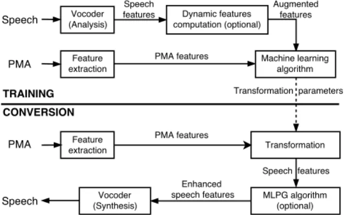
II. STATISTICALARTICULATORY-TO-SPEECHMAPPING This section details the proposed techniques for generating audible speech from captured articulator movement. A block-diagram of the general scheme applied for this transformation is illustrated in Fig. 1. There are two stages: a training stage where the transformation parameters are learned from parallel speech and PMA data and a conversion stage in which speech is synthesised from PMA data only. Initially, we consider GMMs to represent the articulatory-to-acoustic mapping, as described in Section II-A. Next, we extend, in Section II-B, this mapping technique by replacing the GMMs by DNNs. Finally, in Section II-D, we describe the mapping using RNNs,

(3)

Fig. 1: Block-diagram of the general scheme proposed for mapping the articulator movement into audible speech, includ-ing both traininclud-ing and conversion stages.

which explicitly accounts for the temporal evolution of the signals.

A. Conventional GMM-based mapping technique

The GMM-based mapping technique was originally pro-posed in [26] for VC and later applied to both articulatory-to-acoustic and acoustic-to-articulatory problems in [8], [30]. Here, we apply it to our articulatory-to-acoustic mapping problem. Firstly, we denote byxtandytthe source and target

feature vectors at time frame t, with dimensions Dx andDy

respectively, computed from the PMA and speech signals. In Section III-A3 we give the details of how these vectors are extracted from the raw signals. Mathematically, the aim of this technique is to model yt = f(xt), where the mapping

function f(·) is known to be non-linear [31]. Depending on the capabilities of the sensing device, this function might also be non-unique if the same sensor data can be obtained for different articulatory gestures (e.g. if the SSI is not able to capture the movement of some vocal-tract areas well).

To represent the articulatory-to-acoustic mapping, a GMM is used. As shown in Fig. 1, the dynamic speech features may also be taken into account in order to obtain smooth trajec-tories for the predicted speech features [26]. Only the first derivatives are considered and computed as∆yt=yt−yt−1.

The augmented target vector containing the static and dynamic features is defined as y_t = [y>_t,∆y_t>]>. For later use, we express the linear relation between the sequence of static speech parameters Y = [y₁>, . . . ,y_T>]> and the sequence of augmented speech parameters Y = [y>1, . . . ,y>T]> as Y =

RY, whereR is a(2DyT)-by-(DyT)matrix for computing

the sequence of augmented features vectors from the sequence of static features. More details about the construction ofRcan be found in [26], [27].

Let D = {zi} with i = 1, . . . , N represent the parallel

dataset with the feature vectors extracted from the training signals and z = [x>,y>]> is the concatenation of the source and target vectors. To learn the mapping between source and augmented target feature vectors, the expectation-maximisation (EM) algorithm is used in the training stage to fit

a GMM with the joint distributionp(x,y)toD. The resulting probability density function (pdf) has the following form

p(z) =p(x,y) = K

X

k=1

π(k)N(z;µ(k)_z ,Σ(k)_z ). (1)

The parameters of the GMM are the mixture weightsπ(k), mean vectorsµ(k)z = [µ(k)

>

x ,µ(k)

>

y ]

>_{and covariance matrices}

Σ(k)_z = "

Σ(k)xx Σ(k)_xy Σ(k)_yx Σ(k)_yy

#

for each Gaussian componentk= 1, . . . , K in the GMM. In the conversion stage, as illustrated in Fig. 1, the most likely sequence of static speech parameters Yˆ = [ ˆy>1, . . . ,yˆ>T]> is predicted from the articulatory features

X = [x>1, . . . ,x>T]>. Rather than estimating the speech

features frame-by-frame, the whole sequence of feature vectors is estimated at once under the constraints of both the static and dynamic speech features. This estimation is carried out by solving the following optimisation problem:

ˆ Y = arg max Y p(Y|X) = arg max Y p(RY|X). (2)

To solve (2), we use the MLPG algorithm with single-mixture approximation described in [26]. The solution to (2) is given by

ˆ

Y = (R>C−1R)−1R>C−1E, (3) where the (2DyT)-dimensional vector E and (2DyT) -by-(2DyT)block-diagonal matrixC are defined as follows,

In these expressions, kˆt = arg max1≤k≤KP(k|xt)

repre-sents the most likely Gaussian component at time t, while µ(k)_y_|_x

t andΣ

(k)

y|xt are the mean vector and covariance matrix of the posterior distributionp(y|xt, k). These parameters can be

easily computed from the parameters of the joint distribution p(x,y|k)as shown e.g. in [32].

From (3), we see that the predicted sequence of speech feature vectors Yˆ is computed as a linear combination of the frame-level speech estimates E in (4) computed from sensor data. In other words, the information provided by each source feature vector affects the reconstruction ofallthe target vectors. There are two covariance matrices involved in the prediction in (3): Σ_{Y Y} =C, which models the frame-level correlations between static and dynamic speech features, and Σ_{Y Y} = (R>C−1_R₎−1_R>_{, which models the correlations} between speech feature vectors at different time instants.

In [26] it is reported that the mapping represented by (3) produces temporal trajectories for the speech parameters that are often over-smoothed in comparison with the trajectories in natural speech. In particular, some detailed characteristics of speech are lost and the synthesised speech sounds muffled compared to natural speech. As discussed in [26], [33] the reason for this over-smoothing effect is the statistical averaging process carried out during GMM training. To alleviate this

(4)

problem, a mapping technique considering the GV of the speech parameter trajectories was proposed in [26]. In this case, the sequence of speech feature vectors is determined as follows ˆ Y = arg max Y {logp(RY|X)ω+ logp(v(Y))}, (6) where ω = 1/2T as suggested in [26], v = [v(1), . . . , v(Dy)]> is the Dy-dimensional vector with the

variances across time of each speech feature (i.e. v(d) = Var(yd

1, . . . , ydT)), and logp(v(Y)) is a new term which

penalises the reduction in variance of the predicted parameter trajectories. In this work, p(v(Y))is modelled as a Gaussian distribution with diagonal covariance matrix.

Unlike (2), there is no closed-form solution to (6) so we solve it iteratively by gradient-based optimisation methods. Finally, as shown in Fig. 1, a speech waveform is generated from the predicted features Yˆ using a vocoder.

B. DNN-based conversion

DNNs have been shown to achieve state-of-the-art per-formance in various speech tasks such as automatic speech recognition [34], speech synthesis [35], [36], voice conversion [37] and articulatory-to-acoustic mapping [6], [19]–[21] as well. Inspired by this, we describe in this section an alternative technique which employs DNNs to represent the mapping between PMA and speech feature vectors. In particular, a DNN is used to directly model the speech-parameter posterior dis-tribution p(y|xt). Here, we assume that the mean ofp(y|xt)

is given by the output of the DNN. To compute its outputs, a DNN uses several layers of nonlinear operations [38]. For a DNN withLhidden layers, the output of thel-th hidden layer at timet is computed as follows

htl =φh(Wlhtl−1+bl), (7)

where Wl and bl are the trainable parameters (i.e. weight

matrix and bias vector) of the l-th hidden layer, φh is a

non-linear activation function, typically the sigmoid function or a rectified linear unit (ReLU) (i.e. φh(z) = max(0,z)). The

first layer is defined as h0

t =xt for allt, while the output is

computed as

y_t=φy(WyhLt +by), (8)

where Wy and by are the weight matrix and bias vector of

the output layer and φy is the output activation function.

For regression problems involving continuous targets (e.g. Mel-Frequency Cepstral Coefficient (MFCC) or continuous F0 prediction) φy is the identity function (i.e. φy(z) = z).

For classification problems with discrete targets (e.g. binary voicing prediction), a logistic sigmoid function, φy(z) = 1/(1 + exp(−z)), is used instead.

Finally, as in the GMM-based mapping, the MLPG algo-rithm in (3) can also be applied to smooth out the predicted speech parameter trajectories E = [y>₁, . . . ,y>_T]>. In this case, the block-diagonal covariance matrix C is given by

C= diag[Σy|x, . . . ,Σy|x

| {z }

Ttimes

], (9)

where Σy|x is computed after the DNN training stage is

completed by estimating the covariance matrix of the squared errors between the original speech features and the DNN predictions over the training examples.

Comparing the GMM and DNN based approaches, we can observe that they differ in the way they approximate the non-linear mapping between source and target vectors. In the GMM-based technique, the mapping is piecewise linearly approximated by splitting the feature space intoKoverlapping regions (one for each mixture component) and approximating the mapping inside each region with a linear operation. The DNN-based technique, on the other hand, uses several layers of nonlinearites which are discriminatively trained using the backpropagation algorithm.

C. Use of contextual information in the GMM/DNN ap-proaches

One shortcoming of the GMM and DNN approaches is that per se they perform an independent mapping for each individual frame, thus ignoring the sequential nature of the PMA and speech signals. To address this limitation, these approaches can use the MLPG algorithm to post-process the frame-level speech parameter predictions to obtain smoother trajectories, as discussed above. However, this comes at the expense of an increased latency in the conversion. For instance, the MLPG algorithm has a latency ofO(T), though a recursive version with less latency has been proposed in [39].

A complementary way to mitigate the frame independence assumption in GMM/DNN approaches is by training these methods with segmental features, which are obtained from symmetric windows with ω consecutive PMA frames. To reduce dimensionality of the segmental features, we apply the partial least squares (PLS) technique [40] in this paper. By using these segmental features, we aim to reduce the uncer-tainty associated with the non-linear, non-unique articulatory-to-acoustic mapping by taking into account more contextual information.

D. Mapping using RNNs

Here, we explore RNNs as a way of modelling the PMA-to-acoustic mapping which explicitly considers the data dynam-ics. An RNN is a type of neural network particularly suited to modelling sequential data with correlations between neigh-bouring frames. In an RNN the outputs at each time instant are computed by (implicitly) considering all the inputs up to that time. To do so, these networks use hidden layers similar to those defined in (7) but modified so that the information in the RNNs not only flows from the inputs to the outputs but also across time instants, as illustrated in Fig. 2a. For a standard RNN with L hidden layers, the following equation is iteratively applied from t = 1 to T and l = 0, . . . , L to compute the outputs of each layer

− → hl_t=φh( −→ Wl − → hl_t−1+−→Vl − → hl_t₋₁+−→bl), (10) where −W→l, − → Vl, and − →

bl are the trainable weights for the l

(5)

yt−1 yt yt+1 · · · −→hL t−1 − → hL t − → hL t+1 · · · · · · · · · · −→h1 t−1 − → h1 t − → h1 t+1 · · · xt−1 xt xt+1 (a) yt−1 yt yt+1 · · · ←−hL t−1 ←− hL t ←− hL t+1 · · · · · · −→hL t−1 − → hL t − → hL t+1 · · · · · · ←−hL−1 t−1 ←− hL−1 t ←− hL−1 t+1 · · · · · · −→hL−1 t−1 − → hL−1 t − → hL−1 t+1 · · · · · · · xt−1 xt xt+1 (b) yt−δ · · · yt · · · −→hL t · · · − → hL t+δ · · · · · · · · · · −→h1 t · · · − → h1 t+δ · · · xt · · · xt+δ (c)

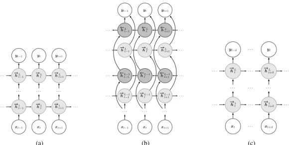
Fig. 2: RNN architectures evaluated in this work. RNNs consist of input and output layers (non-filled nodes) and L hidden layers (shaded nodes). (a) Unidirectional RNN. (b) Bidirectional RNN. (c) Fixed-lag RNN.

that the recursion is applied in the forwarddirection, as such a notation will be useful later. As for the DNNs, we define −

→ h0

t =xt for all t. Likewise, the initial value of the hidden

variables att= 0is−→hl0=0for alll.

Because the RNNs explicitly account for the sequential evolution of speech, there is no need to consider the dynamic speech features as in the GMM and DNN based approaches. Hence, the RNN is trained to directly predict the sequence of static speech parametersY = [y₁>, . . . ,y>_T]>. Similarly to (8), the RNN outputs are computed as

yt=φy( −→ Wy − → hLt + − → by), (11)

where−→hLt is the output of the last hidden layer for frametand

−→ Wy and

− →

by are the trainable parameters of the output layer.

These parameters and those of the hidden layers in (10) are estimated from a parallel dataset containing pairs of source and target vectors using the back-propagation through time (BPTT) algorithm [41], [42].

RNNs as described so far have the problem of explod-ing/vanishing gradients, which prevents them from learning long-term correlations. This problem is solved bygatedRNNs. In a gated RNN, a complex activation function is implemented by means of a state vector,−→hl

t, and two or more multiplicative

operators which act as gates. Fig. 2a shows a time-unrolled gated RNN in which units send the state vector to themselves at the next time instant. Thus, the state vector runs straight down the entire chain of unrolled units while the gates regulate the flow of information to the next time instant (−→hl

t+1) and

to the next layer. Well-known gated RNN architectures are the long short term memory (LSTM) [43], [44] and the GRU [28]. Preliminary experiments showed us that LSTM and GRU units provide roughly the same results on our data, but GRUs are faster to train due to the lower number of parameters. Hence, in the rest of this paper we will only focus on RNNs consisting of GRU blocks. Thus, the hidden activations of the RNN in (10) are instead calculated as the following composite activation function, − →_rl t=σ( −→ Wr_l−→hl_t−1+−→V_lr−→hl_t₋₁+−→br_l) (12) − →_ul t=σ( −→ Wu_l−→hl_t−1+−→V_lu−→hl_t₋₁+−→bu_l) (13) − →_cl t= tanh( −→ Wcl − → hlt−1+ − → Vcl(−→rlt − → hlt−1) + − → bcl) (14) − → hl_t=−→ul_t−→hl_t₋₁+ (1− −→ul_t) −→cl_t (15) where σ is the logistic sigmoid function and represents the element-wise multiplication of two vectors. The key com-ponents of the GRU are the vectors −→r and −→u, which are respectively known as the reset and update gates, and −→c, which is the candidate activation. These gates regulate the flow of information inside the unit and control the update of its hidden state−→h. Finally, the outputsytin a GRU-RNN are

computed just as in standard RNNs, that is, using (11). One limitation of RNNs is that they only make use of the current and past inputs for computing the outputs. For articulatory-to-acoustic conversion, though, the use of future sensor samples could improve the mapping accuracy by tak-ing into account more information about the articulators’ dynamics, at the expense of introducing a certain delay. A popular extension of RNNs that enables this are bidirec-tional RNNs (BiRNNs) [45], which make use of both past and future inputs for computing the outputs by maintaining two sets of hidden sequences: the forward hidden sequence − → H = [−→h1t>, . . . , − → hlt>, . . . , − →

hL_T>]> and thebackward hidden sequence ←H− = [←h−1t>, . . . ,

←− hlt>, . . . ,

←−

hLt>]>. As shown in

Fig. 2b, the backward hidden variables ←h−l

t summarise all

the future information from time T to the current frame t, thus providing complementary information to that summarised in −→hl

t. To compute

←−

H, the following recursive equation is iteratively applied fromt=T to 1 forl= 1, . . . , L:

←− hl_t=φh( ←− Wl ←− hl_t−1+←V−l ←− hl_t+1+←−bl), (16)

where, again, φh is used to denote the GRU composite

activation function in (12)-(15),←−h0

t =xt and

←− hl

(6)

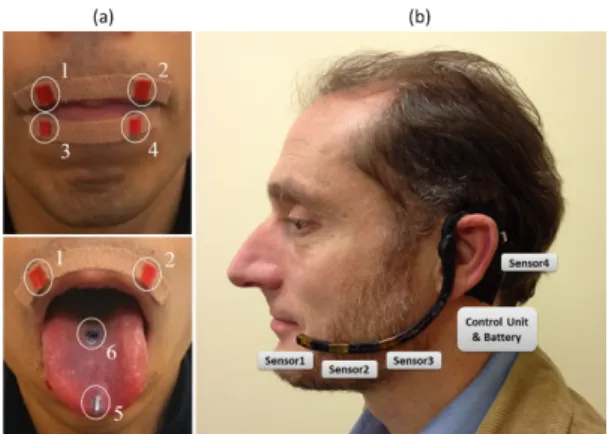
Fig. 3: Permanent Magnet Articulography (PMA) technique for capturing articulator movement. (a) Arrangement of mag-netic pellets on the tongue and lips. Magnet sizes are: 5 mm long by 1 mm diameter (magnets 1-4), 4 mm long and 2 mm diameter (magnet 5) and 1 mm long and 5 mm diameter (magnet 6). (b) Wearable sensor headset with control unit, battery and 4 tri-axial magnetic sensors: Sensor1-3 to measure articulator movements and Sensor4 as a reference sensor to measure the Earth’s magnetic field.

Then, the network outputs are computed from the forward and backward hidden sequences as follows

yt=φy( −→ Wy − → hL_t +←W−y ←− hL_t +by). (17)

Because BiRNNs compute the outputsytin (17) using both

past and future contexts, they could potentially obtain better predictions than unidirectional RNNs. However, it is infeasible to use all the future context in a real-time application. To achieve a good trade-off between the performance achieved by BiRNNs and the latency of unidirectional RNNs, we also investigate the use of fixed-lag RNNs in this work. As shown in Fig. 2c, fixed-lag RNNs are similar to unidirectional RNNs but they also use δ future inputs for computing the outputs, whereδis the size of look-ahead window. To implement fixed-lag RNNs, during the training stage we simply shift the input sequence to the right by addingδnull input vectors (i.e.xt= 0 for t =−(δ−1), . . . ,0) while keeping the output vectors unchanged. Then, the forward hidden sequence and outputs are computed as in a unidirectional GRU-RNN, that is, using (12)-(15) and (11), respectively. This way, during the RNN evaluation, the output vector at timetis obtained using all the inputs up to time t+δ.

III. EXPERIMENTS

To evaluate the performance of the proposed mapping techniques, we performed a set of experiments involving parallel PMA-and-speech data recorded by subjects with nor-mal speaking ability. The performance of the techniques was evaluated objectively using speech synthesiser error metrics and subjectively by means of listening experiments. More details about the evaluation framework are provided below.

A. Evaluation setup

Speaker Sentences Amount of data Average speech rate

M1 420 22 min 173 wpm M2 470 28 min 153 wpm M3 509 26 min 174 wpm M4 519 35 min 133 wpm F1 353 20 min 162 wpm F2 432 22 min 174 wpm

TABLE I: Details of the parallel PMA-and-speech database recorded for the experiments.

1) Data acquisition: Articulatory data was acquired us-ing a bespoke PMA device similar to that in Fig. 3 with magnets temporarily attached to the articulators using tissue adhesive. The headset comprises four anisotropic magneto-resistive sensors: three for measuring articulator movement and one for background cancellation. Each sensor provides 3 channels of data sampled at 100 Hz corresponding to the spatial components of the magnetic field at the sensor location. Contrary to other methods for articulator motion capture, PMA does not attempt to identify the Cartesian position or orientation of the magnets, but rather a composite of the magnetic field from the magnets that are associated with a particular articulatory gesture. As shown in Fig. 3, a total of 6 cylindrical neodymium-iron-boron magnets were used for measuring articulator movement: four on the lips, one at the tongue tip and one on the tongue blade. At the same time as recording sensor data, the subjects’ speech was also recorded at a sampling rate of 48 kHz.

The recording sessions were conducted in an acoustically isolated room. Each session lasted approximately 75 minutes (the maximum time for which the magnet glue is effective). Before the actual data recording, subjects were asked to perform some predefined head movements while keeping their lips and tongue still in order to measure the Earth’s magnetic field. The estimated magnetic field level was then removed from the subsequent PMA samples. During recording, subjects were asked to read aloud sentences from a given corpus (see below for more details). A visual prompt for each sentence was presented to the subject at regular intervals of 10 s.

2) Speech database: For this study we used the Carnegie Mellon University (CMU) Arctic set of phonetically-rich sen-tences [29] because it allows us to evaluate speech recon-struction performance for the full phonetic range. This corpus consists of 1132 sentences selected from English books in the Gutenberg project. Recordings of a random subset of the Arctic sentences were made by 6 healthy British English subjects: 4 men (M1 to M4) and 2 women (W1 and W2). The amount of data recorded by each subject after removing the initial and final silences from the utterances is reported in Table I.

3) Feature extraction: The PMA and speech signals were parametrised as a series of feature vectors computed every 5 ms from 25 ms analysis windows. The speech signals were first downsampled from 48 kHz to 16 kHz and then converted to sequences of 32-dimensional vectors using the STRAIGHT vocoder [46]: 25 MFCCs [47] for representing the spectral envelope, 5-band aperiodicities (0-1, 1-2, 2-4, 4-6, 6-8 kHz), 1 value for the continuous F0 value in logarithmic scale and

(7)

1 value for the binary voiced/unvoiced decision.logF0values

in unvoiced frames were linearly interpolated from adjacent voiced frames.

The 9-channel, background-cancelled PMA signals were firstly oversampled from 100 Hz to 200 Hz to match the 5 ms frame rate. PMA frames are here defined as overlapping segments of data computed every 5 ms from 25 ms analysis windows (same frame rate as for the speech features). For the RNN-based mapping, the models were directly trained with PLS-compressed PMA frames as RNNs are already able to model data dynamics. In PLS, we retained a sufficient number of components to explain 99% of the variance of the speech features. For the GMM and DNN approaches, as mentioned in Section II-C, segmental features computed from the articulatory data were used to train the models. To compute the segmental features, we applied the PLS technique over segments of ω + 4 consecutive PMA samples from the oversampled signal. The segmental feature at time t is computed from a window containing the following: the PMA sample at time t, the d(ω −1)/2e preceding ones and the b(ω−1)/2c+ 4future ones. For example, for ω= 1, 5 PMA samples are concatenated (the current one plus 4 in the future to complete the 25 ms analysis window). For ω= 3, 7 PMA samples are concatenated (1 preceding, the current one and 5 in the future). In the reported experiments we variedωfrom 1 to 31. Finally, the PMA and speech features were normalised to have zero mean and unit variance.

4) Model training and inference: Speaker-dependent mod-els were independently trained for each type of speech feature (MFCCs, 5-band aperiodicities, logF0, and voicing). In the

conversion stage, inference was performed for each type of feature and, finally, the STRAIGHT vocoder was employed to synthesise a waveform from the predicted features.

For the GMM-based mapping of Section II-A, GMMs with 128 Gaussians with full covariance matrices were trained. This number of components was chosen because in our previous work [17] we found that 128-mixtures provided the best results. GMM training was performed with the EM algorithm over 100 iterations. After training, the GMMs for predicting the MFCCs had approximately half a million parameters.

For the DNN approach of Section II-B, models with ap-proximately the same number of parameters as the GMMs were trained: 4 hidden layers and 426 units per layer. The sigmoid activation was used in the hidden layers since it outperformed other activation functions in a set of preliminary experiments. DNN weights were initialised randomly (without pretraining) and optimised using the Adam algorithm [48] with minibatches of size 128 and a learning rate of 0.003. The sum-of-squared errors (SSE) loss was employed for the continuous speech features (i.e. MFCCs, band aperiodicities, andlogF0),

while the cross-entropy loss was employed for the binary voicing decision. We found that applying dropout [49] as a regularization method during training (dropout percentage of 10%) helped the DNNs to generalise better. Training was then run for 100 epochs or until the performance over a validation set dropped.

The training procedure for the RNN mapping in Section II-D was almost identical to that for the DNNs, except that

white noise was added to the inputs (σ2

noise= 0.25) instead of

dropout for regularising the network-weights and minibatches with 50 sentences were used. Similarly, RNNs with 4 hidden layers were trained but we used fewer units per layer (164 GRUs) to end up with approximately the same number of parameters as in the GMM and DNN models.

No smoothing was applied to the voicing parameter trajec-tories in the GMM and DNN approaches, as this was shown ineffective in [30]. Therefore, the frame-level predictions obtained by those models were directly used without any further post-processing. Similarly, as also suggested in [30], the GV penalty was only considered for the conversion of the MFCC features since its effectiveness in the conversion of the excitation features is limited.

5) Performance evaluation: We used a 10-fold cross-validation procedure to evaluate the mapping techniques. In each round of the cross-validation, the total amount of the available data for each speaker is divided into 80% training, 10% validation, and 10% test. The results obtained for the 10 rounds were finally averaged.

The performance of the mapping techniques was evaluated using both objective and subjective quality measures. Accu-racy of spectral estimation was objectively evaluated using the Mel-cepstral distortion (MCD) metric [50] between the MFCCs from the speech signals recorded by the subjects and those estimated from PMA data. For the excitation parameters, we computed the root mean squared error (RMSE) for mea-suring the estimation accuracy of the 5-band aperiodicities, the error rate for the voicing parameter and the Pearson cor-relation coefficient between the estimated and originallogF0

contours in the voiced segments. For subjective evaluation, we conducted a set of listening tests whose details are provided below.

B. Results

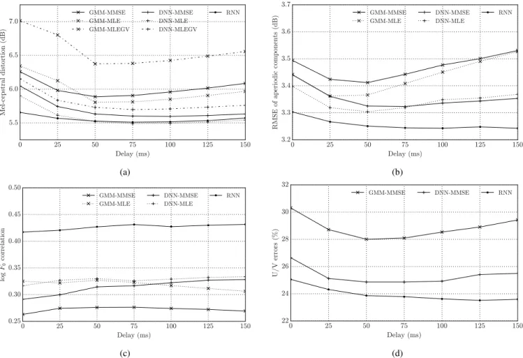
1) Objective results: Fig. 4 shows the objective distortion metrics between the speech signals recorded by the subjects and those estimated from PMA data by the mapping tech-niques. These techniques are the baseline GMM- and DNN-based mapping techniques with frame-level speech-parameter predictions and no smoothing (GMM-MMSE and DNN-MMSE), their respective enhanced versions using the MLPG algorithm to smooth out the speech parameter trajectories (GMM-MLE and DNN-MLE), the versions considering both the MLPG algorithm and the GV penalty (GMM-MLEGV and DNN-MLEGV) and, finally, the mapping technique based on fixed-lag RNNs1_{. For the GMM- and DNN-based techniques,} the performance achieved when using segmental input features computed from symmetric windows spanning from 5 ms of data (0 ms look-ahead window) up to 305 ms of data (150 ms look-ahead window) is shown. For the RNN-based mapping, the results obtained by using look-ahead windows with0(0 ms latency) up to 30 frames (150 ms latency) are reported. Results in Fig. 4 are presented as a function of the delay incurred

1_{Speech samples produced by these techniques are available at https:}

(8)

0 25 50 75 100 125 150 Delay (ms) 5.5 6.0 6.5 7.0 Mel-cepstral distortion (dB) GMM-MMSE GMM-MLE GMM-MLEGV DNN-MMSE DNN-MLE DNN-MLEGV RNN (a) 0 25 50 75 100 125 150 Delay (ms) 3.2 3.3 3.4 3.5 3.6 3.7

RMSE of aperiodic components (dB)

GMM-MMSE GMM-MLE DNN-MMSE DNN-MLE RNN (b) 0 25 50 75 100 125 150 Delay (ms) 0.25 0.30 0.35 0.40 0.45 0.50 lo g F0 c or re la ti on GMM-MMSE GMM-MLE DNN-MMSE DNN-MLE RNN (c) 0 25 50 75 100 125 150 Delay (ms) 22 24 26 28 30 32 U/V errors (%) GMM-MMSE DNN-MMSE RNN (d)

Fig. 4: Average objective results for all subjects computed between the original speech features and those estimated from PMA data by using the mapping techniques described in Section II and considering equivalent delays from0to150ms for segmental feature computation and look-ahead: a) Speech spectral envelope distortion (MCD), b) aperiodic component distortion (5-band RMSE), c) speech fundamental frequency (log F0 correlation), and d) unvoiced/voiced decision accuracy (frame error rate).

when computing the segmental features (GMM-MMSE, DNN-MMSE conversion techniques) or due to the use of future PMA samples in the look-ahead windows (RNN). It must be noted that the actual latency of the techniques employing the MLPG algorithm does not correspond with this delay. For these the actual latency is much higher, typically of the order of the length of the utterance.

Fig. 4 shows that the neural network approaches consis-tently outperform the GMM-based mapping for all the speech features: spectral envelope (Fig. 4a), aperiodic component dis-tortion (Fig. 4b), fundamental frequency (Fig. 4c) and voicing decision (Fig. 4d). Also, it can be seen that the smoothing carried out by the MLPG algorithm (MLE) improves the map-ping accuracy for the spectral envelope and the aperiodicity components, as well as increasing the correlation in the F0

contours. The introduction of the GV penalty, however, seems to degrade the spectral envelope estimation as shown in Fig. 4a (as explained above, this penalty is only considered here for the mapping of the MFCCs). Nevertheless, as discussed below, although it has a negative impact on the objective measures, the GV penalty improves the perceptual quality of speech.

Best results are clearly obtained by the fixed-lag

RNN-based mapping, particularly for the excitation related features (aperiodic components,F0contour and voicing decision). The

PMA technique does not capture any information about the glottal area, so these features must ultimately be predicted from the the lips and tongue movements. In this sense, RNNs seem to be better at exploiting suprasegmental clues to predict these features with a longer time span.

Increasing the window size for computing the segmental features used in the GMM and DNN approaches has a positive effect up to certain point, but excessively long windows can degraded performance. This could be explained by the loss of information produced after applying dimensionality reduction over such a long segmental vectors. A similar, but weaker, effect can be observed for the fixed-lag RNNs.

Fig. 5 shows the MCD results of the RNN-based mapping for each speaker. The results obtained by the BiRNN-based mapping are also included as a reference (since using all the future context is infeasible for a real-time application). The lowest distortions are achieved for male speakers, particularly for M4. The gender differences could be explained by a better fit between the speaker’s vocal tract and the PMA device in terms of size and sensor distribution. Another possible reason

(9)

0 25 50 75 100 125 150 BiRNN Look ahead (ms) 5.0 5.5 6.0 6.5 Mel-cepstral distortion (dB) W1 W2 M1 M2 M3 M4

Fig. 5: MCD results obtained by the fixed-lag RNN- and BiRNN-based mapping approaches for each of the speakers considered in this study.

Vowel Plosive Nasal Fricative Affricate Approximant 0 2 4 6 8 10 Mel-cepstral distortion (dB) Manner of Articulation

Bilabial Labiodental Dental Alveolar Postalveolar Palatal Velar Glottal 0 2 4 6 8 10 Mel-cepstral distortion (dB) Place of Articulation

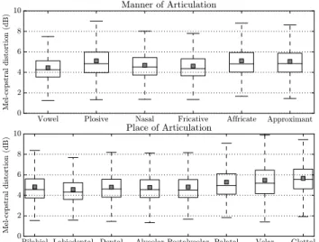
Fig. 6: Distribution of the MCD results obtained by the RNN-based mapping technique with 50 ms look-ahead for different phone categories. Each box represent the first quartile (lower edge), median (segment inside the box) and third quartile (upper edge of the box) of the MCD distribution for each phonetic class, while the small shaded squares inside the boxes represent the means of the distributions. (Upper) Distribution of MCD results for all speakers when considering the manner of articulation. (Lower) MCD distribution for the place of articulation categories.

for these differences comes from the fact that speaker M4 recorded more training data (35 minutes compared to around 25 minutes for the other subjects), and took care to speak slowly (133 words per minute compared to an average of 174 for the other speakers) and clearly. It can be concluded that a delay of 50ms provides a reasonable compromise between speech quality and the mental stress which such a delay might induce in the speaker. Thus, in the following, we will focus on fixed-lag RNNs with a look-ahead set to this value.

Fig. 6 shows two boxplots with the MCD results for the RNN-based mapping (look-ahead of 50 ms) for different pho-netic categories. To compute these results, the speech signals were first segmented into phones by force-aligning their

word-level transcriptions using an ASR system adapted to each subject’s voice. The phone-level transcriptions were then used to segment the original and estimated speech signals. Next, the MCD metric was computed for each phone in English. For the sake of clarity of presentation, we show the aggregated results computed for those phones sharing similar articulation properties. When considering the manner of articulation, it can be seen that the vowels and fricatives (with median values of 4.25 ± 0.005 dB and 4.37 ± 0.009 dB, with p < 0.05) are the best synthesised sounds, while plosive, affricate and approximant consonants (whose medians are, respectively, 4.85 ± 0.009 dB, 4.82 ± 0.028 dB and 4.85 ± 0.012 dB, withp <0.05) are, on average, less well reconstructed due to their more complex articulation and dynamics. For the place of articulation classes, we see that the phones articulated at the middle and back of the mouth (i.e. palatal, velar and glottal consonants, whose MCD median values are 4.96±0.039 dB, 5.19 ± 0.019 dB and 5.55 ± 0.027 dB with p < 0.05) are systematically more poorly estimated. This is due to those areas of the vocal tract not being well captured by PMA [17], [51].

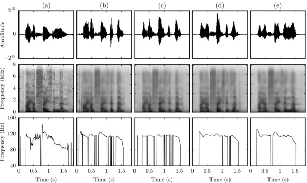
Finally, in Fig. 7, examples of speech waveforms and speech features are shown for natural speech and speech synthesised with several mapping techniques. It can be seen that all techniques are able to estimate the speech formants relatively well, but they are more sharply defined and their trajectories more stable in the RNN- and BiRNN-based estimates. This is not the case of the suprasegmental features (i.e.F0and

voic-ing), where the GMM-MLE and DNN-MLE methods show many errors when predicting the voicing feature. Also, the estimated F0 contours are much flatter than the natural ones.

In contrast, the RNN approaches more accurately predict these features due to their ability to model long-term correlations as commented before. Particularly remarkable is theF0 contour

estimated by the BiRNN technique from PMA data, as PMA does not make any direct measurement ofF0. It is also worth

noting that some detailed characteristics present in natural speech are lost in the spectrograms obtained by the mapping techniques. The reason is that these characteristics are related to articulatory movements which the current PMA device is not yet able to capture.

2) Subjective results: We conducted several listening tests to evaluate the naturalness, quality and intelligibility of the speech produced by the mapping techniques. The details of each listening test and the results obtained are reported next.

First, we conducted an AB test to evaluate the naturalness of different types of excitation signal for the speech predicted from sensor data. Because of the limited ability of PMA to capture information from the vocal folds, we wanted to determine which type of excitation signal sounds more natural when predicted from sensor data. The four types of excitation signals we evaluated are:

• Whispered speech, i.e. speech synthesised without voic-ing.

• Monotone F0: a fixed F0 value (the average F0 for

each speaker) is used for speech synthesis. For speech synthesis we use the aperiodicities and voicing estimated from the sensor data.

(10)

−215 0 215 Amplitude

(a)

(b)

(c)

(d)

(e)

0 2 4 6 8 Frequency (kHz) 0 0.5 1 1.5 Time (s) 40 80 120 160 Frequency (Hz) 0 0.5 1 1.5 Time (s) 0 0.5 1 1.5 Time (s) 0 0.5 1 1.5 Time (s) 0 0.5 1 1.5 Time (s)

Fig. 7: Examples of speech waveforms (first row), spectrograms (second row) and F0 contours (third row) for the sentence

‘I had faith in them’ for (a) natural speech and speech predicted by the following mapping techniques: (b) GMM-MLE, (c) DNN-MLE, (d) RNN with look-ahead of 50 ms and (e) BiRNN. For the GMM-MLE and DNN-MLE methods, segmental features computed over segments spanning 205 ms of data are employed.

Whispered Monotone F0 Cont. F0 Cont. F0

(all voiced) 0 20 40 60 80 100 Preference score (%) 95% confidence interval

Fig. 8: Results of the listening test on naturalness of different types of excitation signal.

• Continuous F0: all the excitation parameters (i.e. F0,

band aperiodicities and unvoiced/voiced (U/V) decision) are estimated from sensor data.

• ContinuousF0(all voiced): as can be deduced from Fig.

4d, the estimation of the voicing parameter from sensor data is currently far from perfect. The errors in the voicing prediction can degrade the perceptual speech quality, so to avoid this, we also evaluate an excitation signal with a continuousF0 contour but all the sounds are synthesised

as voiced.

Twelve listeners participated in the AB test. In the test, the listeners were presented with two versions of the same speech sample but resynthesised with different types of excitation signals and asked to select the version they preferred in terms

Reference Anchor DNN-MMSE DNN-MLEDNN-MLEGV RNN 0 20 40 60 80 100 MUSHRA score [0-100] 95% confidence interval

Fig. 9: Results of the listening test on speech quality.

of naturalness. Each listener evaluated 60 sample pairs: 10 samples for each of the 6 types of excitation signal. All the speech samples were synthesised by the RNN-based technique with look-ahead of 50 ms. The results of the test are shown in Fig. 8. Clearly, speech signals synthesised with Continuous F0and U/V decision are considered significantly more natural

than the other types of excitation. The next more natural types of excitation are the Continuous F0 and all the sounds

voiced and, surprisingly, the Whispered excitation. Least nat-ural, although not significantly different from the Whispered excitation under the sample considered, is the Monotone F0

excitation, which most of the listeners considered very robotic. Next, we conducted a MUlti Stimulus test with Hidden Ref-erence and Anchor (MUSHRA) [52] test to evaluate the speech

(11)

quality resulting from the DNN- and RNN-based mappings. The GMM-based mappings were not evaluated since they obtained the worst objective results and we preferred not to overwhelm the listeners with an excessive number of stimuli to rate. 18 listeners participated in the test and each one assessed 10 different items randomly chosen from a set of available synthesised utterances. For each item, the listeners evaluated speech samples generated by the DNN-MMSE, DNN-MLE, DNN-MLEGV, and RNN approaches in comparison with a reference and an anchor stimuli. For the DNN approaches, a symmetric window with 21 frames (i.e. look-ahead window of 10 frames, that is, 50 ms) was used. For the RNN approaches, the same look-ahead window was used. The signals resynthe-sised with the STRAIGHT vocoder were used as a reference while a GMM-MMSE mapping poorly represented with only 16 Gaussians and no segmental features was employed for the anchor. All the speech samples were synthesised with the Continuous F0 and U/V decision excitation since this

configuration yielded the highest naturalness scores in Fig. 8.

Figure 9 summarises the results of the MUSHRA test. As expected, the Reference and Anchor systems achieved, respectively, the best and worst scores. Despite the objec-tive distortion metrics in Fig. 4, the DNN-MLEGV method achieves significantly higher quality scores than the DNN-MLE method. Thus, the GV penalty seems to improve the perceived quality of speech. On the other hand, in agreement with the objective distortion metrics, the RNN technique achieves significant better results than the DNN-MMSE and DNN-MLE methods and provides a speech quality comparable to DNN-MLEGV but without incurring its long latency. There are no significant differences between the DNN-MMSE and DNN-MLE methods in terms of speech quality.

Finally, we conducted a subjective evaluation of speech intelligibility resulting from the following techniques: GMM-and DNN-based techniques with the MLE GMM-and MLEGV con-version algorithms and the fixed-lag RNN-based mapping. For the listening test, we made a selection of the Arctic sentences to avoid those containing proper names, unusual words or unusual constructions in order to evaluate intelligibility in a vocabulary closer to that a laryngectomee might use in her/his daily life. This resulted in a subset of 145 sentences. As in the previous tests, the speech samples were synthesised with the Continuous F0 and U/V excitation. Moreover, to evaluate

the effect of excitation prediction errors on the intelligibility, we also evaluated the intelligibility of speech generated by the RNN method but with whispered excitation. A total of 21 listeners participated in this listening test. Each one was asked to transcribe 9 samples for each of the 6 conversion systems above (i.e. 54 samples in total). Listeners were allowed to replay the speech stimuli as many times as they wanted.

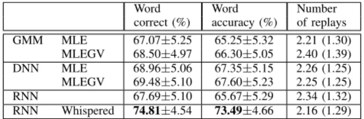
Table II shows the results of the intelligibility test. Three measures are reported for each technique: the percentage of words correctly identified by the listeners (word correct), the word accuracy (i.e. ratio of words correctly identified after discounting the insertion errors) and the average number of replay times by the listeners. The differences in results obtained are not statistically significant in our sample, but it

Word Word Number

correct (%) accuracy (%) of replays GMM MLE 67.07±5.25 65.25±5.32 2.21 (1.30) MLEGV 68.50±4.97 66.30±5.05 2.40 (1.39) DNN MLE 68.96±5.06 67.35±5.15 2.26 (1.25) MLEGV 69.48±5.10 67.60±5.23 2.25 (1.25) RNN 67.69±5.10 65.67±5.29 2.34 (1.32) RNN Whispered 74.81±4.54 73.49±4.66 2.16 (1.29) TABLE II: Results of the intelligibility test (average results for all speakers). 95% confidence intervals for the means are reported for the word correct and word accuracy results. For the number of replays, the average number of replays and standard deviation (SD) are shown.

Word Word Number

correct (%) accuracy (%) of replays GMM MLE 80.15±8.76 79.18±8.76 1.82 (1.06) MLEGV 82.60±6.49 79.96±6.67 2.10 (1.20) DNN MLE 84.65±6.92 83.49±6.92 1.69 (0.90) MLEGV 81.33±6.86 80.34±6.98 1.87 (1.12) RNN 87.53±4.88 86.53±4.98 1.84 (1.06) RNN Whispered 92.00±3.41 91.53±3.57 1.64 (1.13) TABLE III: Results of the intelligibility test for the speaker M4.

can be seen that they follow the same trend as for the objective results: the neural network based approaches outperform the GMM-based mapping and, as in the results of the speech quality test, the GV penalty seems to be beneficial for both GMM- and DNN-based mappings.

Table III shows the intelligibility results for M4, the speaker who achieved the best objective results in Fig. 5. Surprisingly, although the whispered excitation was ranked among the less natural excitations in Fig. 8, the best intelligibility results for this speaker are obtained using the RNN method with this type of excitation. A similar finding has been reported by other authors for a non-audible murmur (NAM)-based SSIs [30] and it is also apparent from the average results in Table II (although not statistically significant). This can be attributed to the errors made during the estimation of the voiced excitation signal hampering the understanding of the converted signal. For the rest of the mapping techniques, a similar trend to that mentioned above for all speakers can be observed. To our knowledge both the objective and subjective results for this speaker are the best obtained for a silent speech interface, and, furthermore, they are obtained without a restricted vocabulary and with an unobtrusive device that delivers audio in close to real time.

IV. CONCLUSIONS

In this paper we have presented a technique for synthesising audible speech from sensed articulator movement using a tech-nique known as PMA. To estimate the transformation between PMA data and speech acoustics, three types of supervised machine learning techniques have been investigated: Gaus-sian mixture models (GMMs), deep neural networks (DNNs) and recurrent neural networks (RNNs). These techniques are trained on parallel data to learn the mapping between the articulatory data and the speech parameters from which a

(12)

waveform signal is finally synthesised. We have reported that each machine learning technique has different latency requirements, an important parameter that has to be taken into account for our ultimate goal in this work: real-time speech restoration for larygectomees.

Results have been reported for two types of evaluations on a parallel database with speech and articulatory data recorded by 6 British-English healthy speakers: objective quality metrics and three listening tests. From the objective evaluation, it is clear that the best performance is obtained using BiRNNs for the mapping. This technique, however, cannot be implemented in real-time and, hence, it could not be applied for real-time PMA-to-speech conversion, but it could potentially be used for batch processing. Encouragingly, a related architecture, a fixed-lag RNN that introduces a small latency by exploiting some sensor samples in the future, has been shown to achieve similar results to that of the BiRNN architecture. Evaluations of latency in data acquisition, transformation and synthesis indicate that these are small and so this approach could enable a real-time speech synthesis with latencies of 25-50 ms.

The results of a listening test on speech naturalness have shown that, despite the PMA devices’ inability to deliver any voicing information, a voiced glottal signal can be estimated from the articulatory data, which improves the perceptual naturalness of the speech produced by the mapping techniques. Nevertheless, in terms of intelligibility, a listening test con-cluded that the intelligibility of signals synthesised with a white-noise excitation (i.e. a whispered voice) are far more intelligible than other types of excitation signal. This can be attributed to the errors in the F0 and voicing estimation from

PMA data. The intelligibility of our best mapping method on a phonetically rich task is, on average, around 75% words correctly identified, but it can reach accuracies around 92% for some speakers.

There is still work to be done before the techniques psented in this paper can be applied to help laryngectomees re-cover their voices (our ultimate goal). Firstly, a subject-tailored design of the PMA device must be developed to achieve more consistent results across individuals. Also, there are parts of the vocal tract that the PMA device is not accurately sensing (e.g. glottis and velum) and the performance of the proposed techniques could be greatly improved by modelling these areas. Another interesting topic for future research would be that of adding more constraints for the articulatory-to-acoustic mapping since, apart from the dynamics constraints in the RNNs, few constraints are imposed. In this sense, the introduction of linguistic knowledge could help to improve the performance by constraining more the mapping process. Another interesting topic of research is that of investigating ways of speaker adaptation for articulatory-to-acoustic map-ping. Finally, our experiments have been based on parallel sensor and acoustic data, but it may not be possible to obtain such data directly in clinical use. Ideally, the magnets would be implanted and recordings made from a patient before removal of the larynx, but when this is not possible we might be able to record acoustics and later on obtain the corresponding sensor data by asking the patient to mime to her/his recordings, with the magnets in place. A variant on this, which would work

for someone who has already had a laryngectomy, would be to mime to another voice. Finally, if the patient can produce speech from an electrolarynx we could deconvolve this signal to obtain articulatory tract parameters from which to estimate more natural acoustics.

ACKNOWLEDGMENT

This is a summary of independent research funded by the National Institute for Health Research (NIHR)’s Invention for Innovation Programme (Grant Reference Number II-LB-0814-20007). The views expressed are those of the author(s) and not necessarily those of the NHS, the NIHR or the Department of Health.

REFERENCES

[1] B. Denby, T. Schultz, K. Honda, T. Hueber, J. Gilbert, and J. Brumberg, “Silent speech interfaces,”Speech Commun., vol. 52, no. 4, pp. 270–287, Apr. 2010.

[2] J. S. Brumberg, A. Nieto-Castanon, P. R. Kennedy, and F. H. Guenther, “Brain-computer interfaces for speech communication,” Speech Com-mun., vol. 52, no. 4, pp. 367–379, Apr. 2010.

[3] C. Herff, D. Heger, A. de Pesters, D. Telaar, P. Brunner, G. Schalk, and T. Schultz, “Brain-to-text: decoding spoken phrases from phone representations in the brain,”Frontiers in Neuroscience, vol. 9, no. 217, Jun. 2015.

[4] T. Schultz and M. Wand, “Modeling coarticulation in EMG-based continuous speech recognition,” Speech Commun., vol. 52, no. 4, pp. 341–353, Apr. 2010.

[5] M. Wand, M. Janke, and T. Schultz, “Tackling speaking mode varieties in EMG-based speech recognition,”IEEE Trans. Bio-Med. Eng., vol. 61, no. 10, pp. 2515–2526, Oct. 2014.

[6] L. Diener, C. Herff, M. Janke, and T. Schultz, “An initial investigation into the real-time conversion of facial surface EMG signals to audible speech,” inProc. EMBC, 2016, pp. 888–891.

[7] M. J. Fagan, S. R. Ell, J. M. Gilbert, E. Sarrazin, and P. M. Chapman, “Development of a (silent) speech recognition system for patients following laryngectomy,”Med. Eng. Phys., vol. 30, no. 4, pp. 419–425, 2008.

[8] T. Toda, A. W. Black, and K. Tokuda, “Statistical mapping between articulatory movements and acoustic spectrum using a Gaussian mixture model,”Speech Commun., vol. 50, no. 3, pp. 215–227, Mar. 2008. [9] T. Hueber, E.-L. Benaroya, G. Chollet, B. Denby, G. Dreyfus, and

M. Stone, “Development of a silent speech interface driven by ultrasound and optical images of the tongue and lips,”Speech Commun., vol. 52, no. 4, pp. 288–300, 2010.

[10] J. A. Gonzalez, L. A. Cheah, P. D. Green, J. M. Gilbert, S. R. Ell, R. K. Moore, and E. Holdsworth, “Evaluation of a silent speech interface based on magnetic sensing and deep learning for a phonetically rich vocabulary,” inProc. Interspeech, 2017, pp. 3986–3990.

[11] T. M. Jones, M. De, B. Foran, K. Harrington, and S. Mortimore, “La-ryngeal cancer: United Kingdom national multidisciplinary guidelines,”

J. Laryngol. Otol., vol. 130, no. Suppl 2, pp. S75–S82, 2016.

[12] J. M. Gilbert, S. I. Rybchenko, R. Hofe, S. R. Ell, M. J. Fagan, R. K. Moore, and P. Green, “Isolated word recognition of silent speech using magnetic implants and sensors,”Med. Eng. Phys., vol. 32, no. 10, pp. 1189–1197, 2010.

[13] R. Hofe, S. R. Ell, M. J. Fagan, J. M. Gilbert, P. D. Green, R. K. Moore, and S. I. Rybchenko, “Small-vocabulary speech recognition using a silent speech interface based on magnetic sensing,” Speech Commun., vol. 55, no. 1, pp. 22–32, 2013.

[14] A. Toutios and S. Narayanan, “Articulatory synthesis of french connected speech from EMA data,” inProc. Interspeech, 2013, pp. 2738–2742. [15] M. Speed, D. Murphy, and D. Howard, “Modeling the vocal tract transfer

function using a 3d digital waveguide mesh,”IEEE/ACM Trans. Audio

Speech Lang. Process., vol. 22, no. 2, pp. 453–464, 2014.

[16] J. L. Kelly and C. C. Lochbaum, “Speech synthesis,” Proc. of the

Stockholm Speech Communication Seminar, 1962.

[17] J. A. Gonzalez, L. A. Cheah, J. M. Gilbert, J. Bai, S. R. Ell, P. D. Green, and R. K. Moore, “A silent speech system based on permanent magnet articulography and direct synthesis,”Comput. Speech Lang., vol. 39, pp. 67–87, 2016.

(13)

[18] T. Hueber and G. Bailly, “Statistical conversion of silent articulation into audible speech using full-covariance HMM,”Comput. Speech Lang., vol. 36, pp. 274–293, 2016.

[19] S. Aryal and R. Gutierrez-Osuna, “Data driven articulatory synthesis with deep neural networks,”Comput. Speech Lang., vol. 36, pp. 260– 273, 2016.

[20] F. Bocquelet, T. Hueber, L. Girin, P. Badin, and B. Yvert, “Robust articulatory speech synthesis using deep neural networks for BCI ap-plications,” inProc. Interspeech, 2014.

[21] F. Bocquelet, T. Hueber, L. Girin, C. Savariaux, and B. Yvert, “Real-time control of an articulatory-based speech synthesizer for brain computer interfaces,”PLOS Computational Biology, vol. 12, no. 11, p. e1005119, 2016.

[22] A. J. Yates, “Delayed auditory feedback,”Psychological bulletin, vol. 60, no. 3, p. 213, 1963.

[23] A. Stuart, J. Kalinowski, M. P. Rastatter, and K. Lynch, “Effect of delayed auditory feedback on normal speakers at two speech rates,”

J. Acoust. Soc. Am., vol. 111, no. 5, pp. 2237–2241, 2002.

[24] J. M. Gilbert, J. A. Gonzalez, L. A. Cheah, S. R. Ell, P. Green, R. K. Moore, and E. Holdsworth, “Restoring speech following total removal of the larynx by a learned transformation from sensor data to acoustics,”

J. Ac. Soc. Am., vol. 141, no. 3, pp. EL307–EL313, 2017.

[25] L. A. Cheah, J. Bai, J. A. Gonzalez, S. R. Ell, J. M. Gilbert, R. K. Moore, and P. D. Green, “A user-centric design of permanent magnetic articulography based assistive speech technology,” inProc. BioSignals, 2015, pp. 109–116.

[26] T. Toda, A. W. Black, and K. Tokuda, “Voice conversion based on maximum-likelihood estimation of spectral parameter trajectory,”IEEE

Trans. Audio Speech Lang. Process., vol. 15, no. 8, pp. 2222–2235, Nov.

2007.

[27] K. Tokuda, T. Yoshimura, T. Masuko, T. Kobayashi, and T. Kitamura, “Speech parameter generation algorithms for HMM-based speech syn-thesis,” inProc. ICASSP, 2000, pp. 1315–1318.

[28] K. Cho, B. Van Merriënboer, Ç . Gülçehre, D. Bahdanau, F. Bougares, H. Schwenk, and Y. Bengio, “Learning phrase representations using RNN encoder–decoder for statistical machine translation,” in Proc.

EMNLP, 2014, pp. 1724–1734.

[29] J. Kominek and A. W. Black, “The CMU Arctic speech databases,” in

Fifth ISCA Workshop on Speech Synthesis, 2004, pp. 223–224.

[30] T. Toda, M. Nakagiri, and K. Shikano, “Statistical voice conversion techniques for body-conducted unvoiced speech enhancement,” IEEE

Trans. Audio Speech Lang. Process., vol. 20, no. 9, pp. 2505–2517,

Nov. 2012.

[31] B. S. Atal, J. J. Chang, M. V. Mathews, and J. W. Tukey, “Inversion of articulatory-to-acoustic transformation in the vocal tract by a computer-sorting technique,”J. Ac. Soc. Am., vol. 63, no. 5, pp. 1535–1555, 1978. [32] C. M. Bishop, Pattern recognition and machine learning. Springer,

2006.

[33] H. Zen, K. Tokuda, and A. W. Black, “Statistical parametric speech synthesis,”Speech Commun., vol. 51, no. 11, pp. 1039–1064, Nov. 2009. [34] G. Hinton, L. Deng, D. Yu, G. Dahl, A. Mohamed, N. Jaitly, A. Senior, V. Vanhoucke, P. Nguyen, T. Sainath, and B. Kingsbury, “Deep neural networks for acoustic modeling in speech recognition: The shared views of four research groups,”IEEE Signal Process. Mag., vol. 29, no. 6, pp. 82–97, Nov. 2012.

[35] H. Zen, A. Senior, and M. Schuster, “Statistical parametric speech synthesis using deep neural networks,” inProc. ICASSP. IEEE, 2013, pp. 7962–7966.

[36] Z. Wu, C. Valentini-Botinhao, O. Watts, and S. King, “Deep neural networks employing multi-task learning and stacked bottleneck features for speech synthesis,” inProc. ICASSP, 2015, pp. 4460–4464. [37] L.-H. Chen, Z.-H. Ling, L.-J. Liu, and L.-R. Dai, “Voice

conver-sion using deep neural networks with layer-wise generative training,”

IEEE/ACM Trans. Audio Speech Lang. Process., vol. 22, no. 12, pp.

1859–1872, 2014.

[38] Y. LeCun, Y. Bengio, and G. Hinton, “Deep learning,”Nature, vol. 521, no. 7553, pp. 436–444, May 2015.

[39] T. Muramatsu, Y. Ohtani, T. Toda, H. Saruwatari, and K. Shikano, “Low-delay voice conversion based on maximum likelihood estimation of spectral parameter trajectory,” in Proc. Interspeech, 2008, pp. 1076– 1079.

[40] S. De Jong, “SIMPLS: an alternative approach to partial least squares regression,”Chemometrics Intell. Lab. Syst., vol. 18, no. 3, pp. 251–263, 1993.

[41] P. J. Werbos, “Generalization of backpropagation with application to a recurrent gas market model,”Neural Networks, vol. 1, no. 4, pp. 339– 356, 1988.

[42] A. J. Robinson and F. Fallside, “The utility driven dynamic error prop-agation network,” University of Cambridge, Engineering Department, Tech. Rep. CUED/F-INFENG/TR.1, 1987.

[43] S. Hochreiter and J. Schmidhuber, “Long short-term memory,”Neural

computation, vol. 9, no. 8, pp. 1735–1780, 1997.

[44] P. Liu, Q. Yu, Z. Wu, S. Kang, H. Meng, and L. Cai, “A deep recur-rent approach for acoustic-to-articulatory inversion,” in Proc. ICASSP. IEEE, 2015, pp. 4450–4454.

[45] M. Schuster and K. K. Paliwal, “Bidirectional recurrent neural net-works,”IEEE Trans. Signal Process., vol. 45, no. 11, pp. 2673–2681, 1997.

[46] H. Kawahara, I. Masuda-Katsuse, and A. De Cheveigne, “Restructuring speech representations using a pitch-adaptive time–frequency smoothing and an instantaneous-frequency-based F0 extraction: Possible role of a repetitive structure in sounds,”Speech communication, vol. 27, no. 3, pp. 187–207, Apr. 1999.

[47] T. Fukada, K. Tokuda, T. Kobayashi, and S. Imai, “An adaptive algorithm for Mel-cepstral analysis of speech,” inProc. ICASSP, 1992, pp. 137– 140.

[48] D. Kingma and J. Ba, “Adam: A method for stochastic optimization,”

inInternational Conference on Learning Representations, 2015.

[49] N. Srivastava, G. E. Hinton, A. Krizhevsky, I. Sutskever, and R. Salakhutdinov, “Dropout: a simple way to prevent neural networks from overfitting.”J. Mach. Learn. Res., vol. 15, no. 1, pp. 1929–1958, 2014.

[50] R. Kubichek, “Mel-cepstral distance measure for objective speech qual-ity assessment,” inProc. IEEE Pacific Rim Conference on

Communica-tions, Computers and Signal Processing, 1993, pp. 125–128.

[51] J. A. Gonzalez, L. A. Cheah, J. Bai, S. R. Ell, J. M. Gilbert, R. K. Moore, and P. D. Green, “Analysis of phonetic similarity in a silent speech interface based on permanent magnetic articulography,” inProc.

Interspeech, 2014, pp. 1018–1022.

[52] Method for the subjective assessment of intermediate quality levels of