AUC Knowledge Fountain
AUC Knowledge Fountain
Theses and Dissertations
6-1-2015
ADR-Miner: An Ant-based data reduction algorithm for
ADR-Miner: An Ant-based data reduction algorithm for
classification
classification
Ismail Mohamed Anwar Abdel Salam
Follow this and additional works at: https://fount.aucegypt.edu/etds
Recommended Citation Recommended Citation
APA Citation
Abdel Salam, I. (2015).ADR-Miner: An Ant-based data reduction algorithm for classification [Master’s thesis, the American University in Cairo]. AUC Knowledge Fountain.
https://fount.aucegypt.edu/etds/130
MLA Citation
Abdel Salam, Ismail Mohamed Anwar. ADR-Miner: An Ant-based data reduction algorithm for classification. 2015. American University in Cairo, Master's thesis. AUC Knowledge Fountain. https://fount.aucegypt.edu/etds/130
This Thesis is brought to you for free and open access by AUC Knowledge Fountain. It has been accepted for inclusion in Theses and Dissertations by an authorized administrator of AUC Knowledge Fountain. For more
School of Sciences and Engineering
ADR-Miner - An Ant-Based Data
Reduction Algorithm for Classification
A Thesis Submitted to
Department of Computer Science and Engineering
In partial fulfilment of the requirements for
the degree of Master of Science
By
Ismail M. Anwar
Under the Supervision of
Dr. Ashraf M. Abdelbar
ADR-Miner - An Ant-Based Data Reduction Algorithm for Classification
A Thesis Submitted by
Ismail Mohamed Anwar Abdel Salam
To the Master of Science in Computer Science Program March / 2015
In partial fulfillment of the requirements for The degree of Master of Science
Has been approved by
Thesis Committee Supervisor/Chair Affiliation
Thesis Committee Reader/Examiner Affiliation
Thesis Committee Reader/Examiner Affiliation
Thesis Committee Reader/External Examiner Affiliation
I would like to start by thanking Dr. Ashraf Abdelbar for his guidance and patience, for without them this work would not have been possible. I would also like to thank my family and friends for their unyielding support throughout the entire process. To all those who helped me complete this thesis, I sincerely thank you and will forever cherish your support.
Classification is a central problem in the fields of data mining and machine learning. Using a training set of labeled instances, the task is to build a model (classifier) that can be used to predict the class of new unlabeled instances. Data preparation is crucial to the data mining process, and its focus is to improve the fitness of the training data for the learning algo-rithms to produce more effective classifiers. Two widely applied data prepa-ration methods are feature selection and instance selection, which fall under the umbrella of data reduction. For my research I propose ADR-Miner, a novel data reduction algorithm that utilizes ant colony optimization (ACO). ADR-Miner is designed to perform instance selection to improve the predic-tive effecpredic-tiveness of the constructed classification models. Two versions of ADR-Miner are developed: a base version that uses a single classification algorithm during both training and testing, and an extended version which uses separate classification algorithms for each phase. The base version of the ADR-Miner algorithm is evaluated against 20 data sets using three classifica-tion algorithms, and the results are compared to a benchmark data reducclassifica-tion algorithm. The non-parametric Wilcoxon signed-ranks test will is employed to gauge the statistical significance of the results obtained. The extended version of ADR-Miner is evaluated against 37 data sets using pairings from
performance of the classification algorithms but without reduction applied as pre-processing.
Keywords: Ant Colony Optimization (ACO), Data Mining, Classifica-tion, Data Reduction.
Acknowledgements iii
1 Introduction 1
2 Background 7
2.1 Ant Colony Optimization . . . 7
2.1.1 The Ant Colony Optimization Meta-heuristic . . . 9
2.1.2 ACO Algorithms . . . 14 2.1.3 Convergence . . . 20 2.2 Data Reduction . . . 22 2.3 Classification . . . 25 2.3.1 k-Nearest Neighbor . . . 26 2.3.2 C4.5 . . . 27 2.3.3 Naive Bayes . . . 30 3 Related Work 33 3.1 Ant Colony Optimization . . . 33
3.2 Data Reduction . . . 36
4.2 The ADR-Miner Overall Algorithm . . . 44
4.3 Solution Creation . . . 46
4.4 Quality Evaluation and Pheromone Update . . . 49
5 Implementation 51
5.1 ADR-Miner . . . 51
5.2 WEKA Integration . . . 56
6 Experimental Approach 61
6.1 Performance Evaluation and Benchmarking . . . 62
6.2 Effects of Using Different Classifiers During Reduction and
Testing . . . 64
7 Experimental Results 67
7.1 Performance Evaluation and Benchmarking . . . 67
7.2 Effects of Using Different Classifiers During Reduction and
Testing . . . 70
8 Conclusions and Future Work 101
8.1 Conclusions . . . 101
8.2 Future Work . . . 104
Appendix - Pairing Results (Alternate View) 109
2.1 An example of instance selection performed on a data set with
two classes. . . 24
4.1 The ADR-Miner Construction Graph . . . 43
5.1 Materialization of the construction graph in ADR-Miner and
the sliding window of validity during solution construction. . . 53
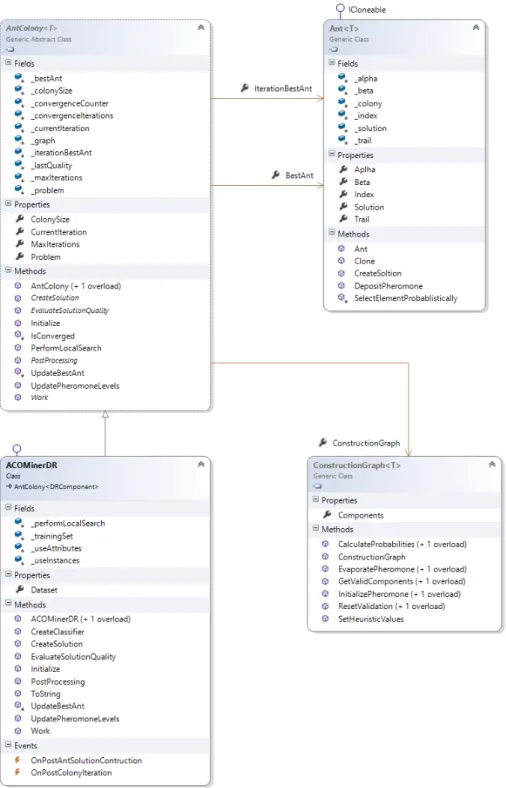
5.2 Class Diagram of ADRMinerDR, AntColony, Ant and
Con-structionGraph. . . 55
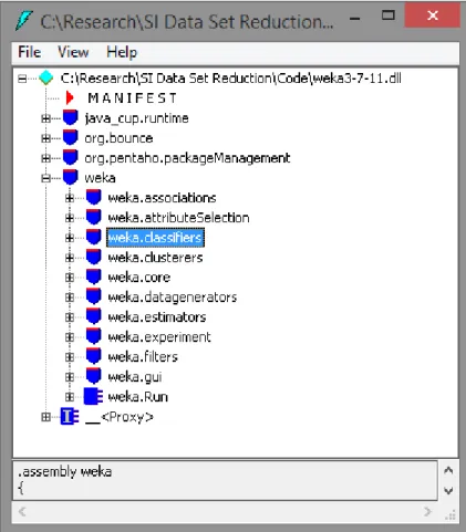
5.3 Disassembly of the weka.dll file. Performed by the Microsoft
IL DASM tool. . . 58
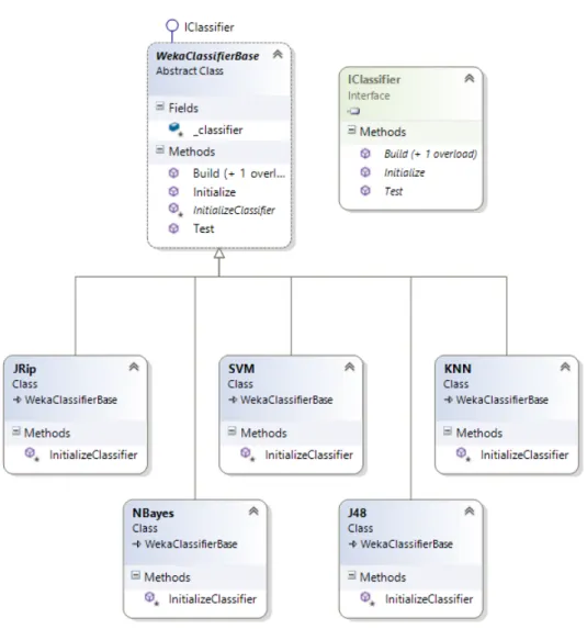
5.4 Class diagram of IClassifier, WekaClassifierBase and all
de-rived classifiers. . . 59
7.1 1-Nearest Neighbor (1-NN) - 1-Nearest Neighbor (1-NN) Results 71
7.2 1-Nearest Neighbor (1-NN) - Na¨ıve Bayes (NB) Results . . . . 72
7.3 1-Nearst Neighbor (1-NN) - Ripper (JRip) Results . . . 73
7.4 1-Nearest Neighbor (1-NN) - C4.5 (J48) Results . . . 74
7.5 1-Nearest Neighbor (1-NN) - Support Vector Machine (SMO)
7.7 Na¨ıve Bayes (NB) - Na¨ıve Bayes (NB) Results . . . 77
7.8 Na¨ıve Bayes (NB) - Ripper (JRip) Results . . . 78
7.9 Na¨ıve Bayes (NB) - C4.5 (J48) Results . . . 79
7.10 Na¨ıve Bayes (NB) - Support Vector Machine (SMO) Results . 80 7.11 Ripper (JRip) - 1-Nearest Neighbor (1-NN) Results . . . 81
7.12 Ripper (JRip) - Na¨ıve Bayes (NB) Results . . . 82
7.13 Ripper (JRip) - Ripper (JRip) Results . . . 83
7.14 Ripper (JRip) - C4.5 (J48) Results . . . 84
7.15 Ripper (JRip) - Support Vector Machine (SMO) Results . . . 85
7.16 C4.5 (J48) - 1-Nearest Neighbor (1-NN) Results . . . 87
7.17 C4.5 (J48) - Na¨ıve Bayes (NB) Results . . . 88
7.18 C4.5 (J48) - Ripper (JRip) Results . . . 89
7.19 C4.5 (J48) - C4.5 (J48) Results . . . 90
7.20 C4.5 (J48) - Support Vector Machine (Support) Results . . . . 91
7.21 Support Vector Machine (SMO) - 1-Nearest Neighbor (1-NN) Results . . . 92
7.22 Support Vector Machine (SMO) - Na¨ıve Bayes (NB) Results . 93 7.23 Support Vector Machine (SMO) - Ripper (JRip) Results . . . 94
7.24 Support Vector Machine (SMO) - C4.5 (J48) Results . . . 95
7.25 Support Vector Machine (SMO) - Support Vector Machine (SMO) Results . . . 96
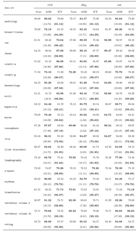
7.1 Experimental Results - Predictive Accuracy % (Size Reduction
%) . . . 68
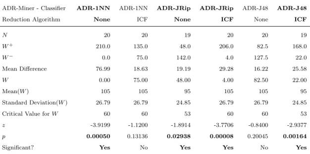
7.2 Results of the Wilcoxon Signed-Rank Test. The ADR-Miner algorithm (paired with a classifier) is compared against the performance of a reducer. . . 70
7.3 Baseline Predictive Accuracy (%) Results for the Classification Algorithms Without Data Reduction . . . 97
7.4 Average Rankings of Predictive Accuracy . . . 98
7.5 Size Reduction (%) Results . . . 99
7.6 Best Performing Combinations . . . 100
8.1 g−hPairing-based Predictive Accuracy (%) Results for ADR-Miner . . . 110
Introduction
Data mining is the process of extracting insightful knowledge from large quantities of data either in an automated or a semi-automated fashion [19], [34]. Data mining techniques have been traditionally divided into four cate-gories: classification, clustering, regression and association rule mining. Clas-sification techniques analyze a given data set and attempt to learn the re-lationship between the input attributes in the data set and a categorical class label. This relationship is then used to build a model that can be used to predict the class label of unforeseen instances. Since the classes for the instances used to build the model are known beforehand, classification is con-sidered to be a form of supervised learning. Clustering is in direct contrast with classification in that it analyzes data sets that have no known class associated with the instances in those data sets. The aim of clustering is to uncover hidden relationships between instances in the data sets being ana-lyzed. In essence, a clustering algorithm will attempt to group the instances in the data set being analyzed into naturally occurring classes, where the instances assigned to a group are ”similar” to one another and ”dissimilar”
to members in other groups. Depending on the clustering algorithm, cluster membership may vary from mutual exclusivity to supporting membership to multiple clusters at the same time. Similarity or dissimilarity in clustering is defined by a distance function - a function that returns the distance between two instances in a data set. As the class labels are not known beforehand, clustering is considered to be a form of unsupervised learning. Regression (and other numerical techniques) are used to build models capable of pre-dicting unseen values in data series that are continuous in nature. Finally, association rule mining analyzes data sets in search of frequently occurring patterns within its instances and attempts to encode these findings in the form of rules. The rules can be used to predict the occurrence of related items when one or more items that are frequently associated with them are detected.
As the work presented in this dissertation is related to classification, let us revisit it and formally define classification. Given a set of labeled instances, the aim of a classification algorithm is to learn the relationship between the input attributes and the label and encode this information as a model. The label associated with each instance defines the class to which the instance belongs, and has to be categorical in nature. If the label is continuous in fashion, then the data mining task used to build models for this label is usually identified as belonging to the regression family of algorithms. The model, as mentioned earlier is used to identify the class of instances that have not been seen by the classification algorithm before. The data set used to learn the model is usually known as the training set. Many techniques have been developed over time to perform classification, and these include
decision trees, classification rules, probabilistic graphical models, instance-based learning, neural networks and support vector machines [5], [8], [25], [34].
With the increasing availability of affordable computational power, abun-dant cheap storage, and the fact that more and more data are starting their life in native digital form, more and more pressure is put on classification algorithms to extract effective and useful models. Real world data sets are frequently rife with noisy, erroneous, outlier, miss-labeled and irrelevant data. These can be harmful to the classification algorithm and, in turn, may affect the predictive power of the produced classification models. In an attempt to remedy these maladies, the data presented to the algorithm for the purposes of training is put through a phase that either removes instances, attributes or both before the actual learning process. This pre-processing phase is known as data reduction. Not only does the data reduction process aim to improve the predictive effectiveness of the produced classifiers by removing the at-tributes and instances that can be misleading to the learning algorithm, it also decreases the size of the training set presented to the algorithm by keep-ing only the most representative instances. The benefits of havkeep-ing a reduced set to work with is two-fold: learning using a smaller volume of data is faster, and the maintenance overhead is diminished.
Ant colony optimization (ACO) [7], [15], [16] is a search meta-heuristic inspired by the behavior of real ants as they forage for food. By observing the ants, it was noted the ants are capable of converging on the shortest path between their nest and the closest food source without any means of
to develop a meta-heuristic that utilizes the same underlying mechanisms to tackle combinatorial optimization problems. Since its introduction, ACO has shown a successful track record with combinatorial optimization problems in multiple fields of application, and has since been extended to handle other types of problems, including data mining problems [38].
In this dissertation I introduce ADR-Miner: an ant-inspired algorithm designed to do data reduction. ADR-Miner adapts ACO to perform data reduction via instance selection with the sole purpose of improving classifier effectiveness. The objective of ADR-Miner is to process a given data set and arrive at the minimum set of instances to use that produces the model with the highest classifier effectiveness. The ADR-Miner algorithm is introduced here in two versions: a base version and an extended one. The base version of ADR-Miner will use a single classification algorithm during both its training and testing phases. The extended version on the other hand will use two separate classification algorithms, one per each phase of the algorithm.
The base version of ADR-Miner will be evaluated using three well known classification algorithms and against 20 data sets from the well-known UCI
Machine-Learning repository. The results obtained will be benchmarked
against the performance of another data reduction algorithm: the Iterative Case Filtering (ICF) algorithm [11]. Statistical significance in the results will be established using the non-parametric Wilcoxon Signed-Rank test. The extended version of ADR-Miner will be evaluated using all the possible pairings between five classification algorithms and against 37 data sets from the UCI repository. The results obtained are then benchmarked against the performance of the five classification algorithms without data reduction.
The rest of this dissertation is structured as follows. Chapter 2 provides a brief introduction to ACO, Data Reduction and Classification. Chapter 3 provides a review the previous work done with ACO and Data Reduc-tion. Chapter 4 presents an in depth explanation of ADR-Miner and its
components. Chapter 5 covers the technical details of implementing the
ADR-Miner algorithm. Chapter 6 covers the experimental approach used to evaluate ADR-Miner, with the results obtained being interpreted in Chapter 7. Finally, I round things off in Chapter 8 with my conclusions and suggested avenues of further research.
Background
In this chapter, we go through the concepts of ACO, classification and data
reduction. These form the core concepts whose intersection is the main
impetus behind the development of ADR-Miner.
2.1
Ant Colony Optimization
Ant colony optimization (ACO) is a search meta-heuristic that is designed to tackle combinatorial optimization problems. First described by Dorigo et al in 1992 [4], ACO is inspired by the behavior observed in multiple species of ants as they forage for food. As the ants forage for food, the scouts would first wander around the opening of the nest looking for a viable food source. As the scouts locate one, they would carry food back to the nest. Over time, it is observed that the ants out searching for food would converge on the shortest
path between the nest and the closest food source. This behavior is not
explicitly wired into the psyche of the individual ants. Instead, the ants only follow a simple set of rules and the resultant property of the ants following
these rules is that the colony displays the capacity of finding the shortest path between it and the closest food source. An individual ant would first start out at the nest, and wander randomly around it favoring paths that have the scent of food. As soon as an ant locates a source of food, it would carry a portion of the food back to the nest. While the ant travels back and forth between the nest and food source, it deposits a chemical, known as a pheromone, along its trail. New ants setting out from the nest would then probabilistically favor paths that contain both scents of pheromone and food on them versus those which do not. As time passes, the pheromone evaporates. Longer paths to the food would have a larger percentage of the pheromone deposited on them evaporate versus shorter paths due to the amount of time an ant takes to traverse this course. As more and more ants find the shortest of the paths favorable, more ants would take this path, all the while depositing pheromone on it further reinforcing its selection in the future. Eventually, all the ants that set out to search and obtain food adopt the shortest path due its highest concentration of pheromone and abandon all the other paths. This emergent behavior of being able to converge on the shortest path between the nest and the food source is what drove Dorigo et al to adapt it into a search meta-heuristic that can be used to solve combinatorial optimization problems.
Over the next few subsections, well will cover how the behavior observed in real life ants was adapted into the ACO search meta-heuristic and some of the most common ACO algorithms in chronological order of development.
2.1.1
The Ant Colony Optimization Meta-heuristic
Before describing the ACO meta-heuristic, let us first deconstruct it into a set of constituent components:
• A construction graph: This is a representation of the search space that
the ants would course in search of a solution. The construction graph is basically a translation of the problem being solved into a form that can be used by the ants. Composed of a set of vertices and edges con-necting them, the construction graph’s vertices represent components that when combined with other vertices in the graph would form a valid solution to the problem being solved. For example, if we are try-ing to solve the Traveltry-ing Salesman Problem (TSP), a given instance of the problem would be translated into a construction graph where the nodes or cities in the instances are directly translated to vertices and the roads connecting them are translated in the edges connecting them. An ant could then start at a city, and construct a valid solution by continuously selecting the next city/vertex to visit till it returns to its starting point. The vertices in a construction graph are also known as decision components, since the ants have to decide to either include or exclude it by choosing whether to visit it or not.
• A fitness function: This is a function that is used to gauge how well a
proposed solution performs in the context of the problem being solved. This is problem specific, and would vary depending on the problem being tackled, whether it is a minimization or maximization type prob-lem. The fitness function is used by the meta-heuristic to determine the fitness of the solutions presented by the ants, and is employed
to determine the best solution encountered throughout the run of the meta-heuristic (and thus return it as the solution to the problem being solved) and is sometimes employed during the pheromone update pro-cedure as elaborated further below. Using TSP as an example, a valid fitness function would be one over the length of the route proposed.
• A colony of ants: This is a collection of agents that share no means of
direct communication with each other and that follow a simple set of rules. These rules dictate the behavior of these agents as they course the construction graph in search of valid solutions.
• A transition probability function: This a function that calculates the
probability for a given decision component on the construction graph for selection from another node on the same graph. This is extensively
used in the Construct Solution() sub-procedure in the meta-heuristic
as will be explained shortly.
• A pheromone update scheme: This describes how the pheromone trails
are updated by the ants as they traverse the construction graph, and how the pheromone evaporates over time.
The overall meta-heuristic shared by most ACO algorithm can be glimpsed in Algorithm 1. The meta-heuristic begins by initializing its parameters and the colony. Depending on the implementation of the meta-heuristic, this can include setting the total number of iterations to be performed, the number of ants in the colony, the number of iterations after which the meta-heuristic is considered to have converged among other possible parameters. The meta-heuristic then enters its main loop (lines 5-9), that only exits when a
pre-defined set of stopping criteria are satisfied. Again, these stopping criteria will depend on the particular implementation of the meta-heuristic, and can range from simple criteria such as exhausting a preset number of iterations to more complex schemes such as detecting stagnation after a number of restarts. Within the main loop, the meta-heuristic goes through three steps: having the ants in the colony construct solutions, applying local search and updating the pheromone trails.
The first step within the main loop is for each ant within the colony
to construct a solution (line 6). This is further expanded in the
Con-struct Solutions() sub-procedure (lines 12-22). To construct a solution, an ant would first start at a node within the construction graph. The beginning node code be a random one or a specific one depending on the problem being solved. From there, the ant would continuously check all feasible neighbors, select the next component from the feasible neighbors and traverse to se-lected component. Once reaching a node with no feasible neighbors, then the ant has basically traversed the construction graph and built a solution. At this point it returns the route it has taken as the solution proposed by that particular ant. Since the selection of components is probabilistic, before a ant selects a node, it will first calculate the probabilities for each node in the feasible neighborhood using the transition probability function and then stochastically select one with a bias towards those with a higher probability. How the ants calculate the probability for each node in their feasible neigh-bors and then proceeds to select one is governed by the implementation’s transition probability function and therefore will differ from one implemen-tation to the other. The transition probability function is a function of two
values: heuristic information available locally to the ants (η) and the amount
of pheromone available at each node (τ). Going with our example of TSP,
one possible value ofη could be 1 divided by the distance from each node to
the next, giving favor of selection towards node that are closer by.
The second step within the main loop of the meta-heuristic is the appli-cation of local search. Here, an attempt is made to improve the fitness of the solutions returned by the ants via the application of a local search algorithm. The algorithm would search in the immediate vicinity of the solution for one with a higher fitness. If such a solution is found, then it would replace the so-lution presented by the ant, otherwise no change is made. This is an optional step, and depending on implementation, it may or may not be applied.
The third and final step within the meta-heuristic’s main loop is the process of updating the pheromone trails. This is done over two phases. First, the ants within the colony would deposit pheromone on the routes they have selected throughout the construction graph. Which ants get to deposit pheromones and how much pheromone is deposited depends on the particular implementation of the meta-heuristic. Generally speaking, the amount of pheromone deposited is usually tied to the fitness of the solutions presented by ants, whether in terms of defining which ants get to deposit pheromones on their routes, or the amount of pheromone deposited per trail. To gauge the fitness of a solution, the meta-heuristic uses the fitness function that is deployed along with the implementation and would therefore differ depending on the type of the problem being solved. Second, the pheromone trails are allowed to evaporate, and as with the process of depositing pheromones is governed by the implementation. Both the deposit and evaporate mechanics
Algorithm 1 General ACO Meta-heuristic
1: procedure ACO Metaheuristic()
2: set parameters
3: initialize colony
4: initialize pheromone trails to τθ
5: repeat
6: Construct Solutions()
7: Apply Local Search() . This step is optional.
8: Update Pheromone Trails()
9: until stopping criteria are satisfied 10: return best solution encountered
11: end procedure
12: procedure Construct Solutions()
13: for each ant in colony do
14: xant ←xant∪Initial Component
15: while valid nodes still exist for ant in construction graphdo
16: N ← get feasible neighbors for ant
17: P ← Get probabilities for each node in N
18: d← Select Component Probabilistically(N,P)
19: xant ←xant∪d
20: end while
21: end for
of the heuristic form part of the pheromone update scheme of the meta-heuristic.
Once the main loop exits, the meta-heuristic returns the best solution encountered. This is the general meta-heuristic that is adhered to by most implementations, and the implementations discussed next are some such ex-amples. For a deeper treatment of the meta-heuristic, the reader is referred to [17].
2.1.2
ACO Algorithms
The number of ACO algorithms has been growing steadily since their in-troduction in the early 1990’s, with extensions and applications emerging for various optimization and data mining problems. In the following subsections, we cover the following algorithms: Ant System, the first and quintessential
ACO algorithm on which meta-heuristic is based; and M AX−M IN Ant
System, an extension on which ADR-Miner is based; Ant Colony System; AS-Rank and Antabu. For a broader coverage of the ACO algorithms, the reader is referred to [15]–[17], [32].
Ant System
The first of the ACO algorithms, Ant System was developed in 1992 [4]. Ant System follows the basic structure of the meta-heuristic described earlier and is in fact what lead to its development. In Ant System, the transition
the following equation: pkij(t) = τα ij(t)η β ij(t) P u∈Nk i(t) τα ij(t)η β ij(t) if j ∈ Nk i (t) 0 if j /∈ Nk i (t) (2.1) where
• τij represents the amount of pheromone deposited on the trail linking
nodei to node j
• ηij represents the a priori effectiveness of moving from nodei to node
j
• α and β represent bias towards pheromone and heuristic information
respectively
• N represents the feasible neighborhood for nodei at time t
An ant at node i would first get its feasible neighborhood N. The feasible
simply represents the nodes the ant can visit next without violating any
problem specific constraints. For each node j in the neighborhood, the ant
would calculate the probability pij and the use Roulette Wheel Selection to
pick a node j from the neighborhood to move to.
The pheromone evaporation and update procedure for Ant System are performed using the following formulas:
τij(t)←(1−ρ)τij (2.2) τij(t+ 1) =τij(t) +4τij(t) (2.3) with 4τij(t) = nk X k=1 4τijk(t) (2.4)
where 4τij(t) = Q f(xk(t)) if link(i, j)∈xk(t) 0 otherwise (2.5)
Here, ρ represents an evaporation factor and ranges between 0 and 1. After
evaporation has been applied, the ant solutions are inspected and for each link in the graph:
• Get all ants that have link(i, j) as part of their solution (xk(t)).
• For each ant in the cohort that include link(i, j) in their solutions,
deposit pheromone in proportion to the quality of the solutions attained
(Equation 2.5). Q is a constant that is set by the user, and Equation
2.5 assumes a minimization problem. For a maximization problem,
Qf(xk(t)) is used instead.
Ant System was first employed by Dorigo et al to solve the Traveling Salesman and the Quadratic Assignment problems, and the algorithm has shown to be successful. The algorithm was later extended, for example by allowing a number of elite ants to deposit an extra amount of pheromones, and was the basis of the ACO meta-heuristic as we know it.
M AX−M IN Ant System
TheM AX−M IN Ant System is an extension of the Ant System algorithm,
and was designed to tackle a specific issue: stagnation. During experimen-tation with Ant System, it was observed the ants would sometimes converge early on a path in the construction graph that might not be optimal and get stuck on a local minima. To remedy this situation, the original Ant System was altered in the following manner:
• Only one ant is allowed to deposit pheromone: The current iteration best or the global best.
• The pheromone levels on the links in the graph are bounded to be
between τmin and τmax.
• Upon initialization, pheromone levels are set to τmax. This is in
con-trast with the Ant System algorithm where the pheromone levels where initialized to zero or a small random figure.
• If and when the algorithm reaches stagnation, the pheromone levels are
reset toτmax.
There are a number of ways to set the values for τmin andτmax. One way
is to set the values for the bounds as static values at the beginning of the algorithm run. Another way, would be to use the following equations based on the best estimation available of the optimal solution:
τmax(t) = ( 1 1−ρ) 1 f(ˆx(t)) (2.6) τmin(t) = τmax(t)(1− √ ˆ pnG) (nG/2−1) √ ˆ pnG (2.7) where
• f(ˆx(t)): the fitness of the best solution encountered so far. This could
be the iteration best or the global best.
• pˆ: the probability of finding the best solution. This is a user set
pa-rameter and ˆp must be less than 1 so that τmin could take on a value
greater than zero.
Note that sinceτmax depends on the best solution found so far, this makes it
time dependent. This results in both bounds forτ being dynamic and adjust
throughout the run of the algorithm.
Ant Colony System
Ant colony system (ACS) is an extension of Ant System that was devel-oped by Dorigo and Gambardella in an attempt to improve performance and achieve a better balance between exploration and exploitation. ACS dif-fers from Ant System on three aspects: the transition probability function, pheromone maintenance and the introduction of the use of candidate lists.
ACS uses Equation 2.8 as its transition probability function. r0 is a user
paremeter set between 0 and 1, while r is a random number generated such
that r∈U(0,1). Using this scheme, an ant will occasionally favor making a
greedy decision to select the node with the highest pheromone and heuristic
values within its feasible neighborhood. At times when r is greater than r0,
then ant would select its next step based on Equation 2.1, but withα preset
to 1. P(i, j) = arg maxu∈Nk j(t){τiu(t)η β iu(t)} if r ≤r0 J otherwise (2.8)
The pheromone trails in ACS are only updated by the best ant, and as in MMAS, this could either be the iteration best or the global best. To hasten evaporation, and promote exploration within the colony, a little amount of pheromone is removed every time an ant visits a node within the graph. Also, as in MMAS, the pheromone levels are bounded between a minimum and a
maximum level to stave off early convergence on local minima.
Candidate lists are preferred nodes to be visited next given an ants posi-tion, and influence how an ant transitions from one node to the next within the graph. Given a choice to select a node, an ant would first inspect the candidate list for choices and make a selection there, before looking into the rest of the feasible neighborhood. Members in the candidate list are usually sorted from highest utility to least, and a candidate list is always less than feasible neighborhood in terms of size.
AS-Rank
AS-Rank is a relatively straight forward extension to Ant System, with mod-ifications introduced to how pheromones are updated, using elitist ants and only allowing the best ant to deposit an extra amount of pheromone. The pheromone update rule in AS-Rank is modified into the following:
τij(t+ 1) = (1−ρ)τij(t) +ne4τˆij(t) +4τijr(t) (2.9) where 4τˆij(t) = Q f(ˆx(t)) (2.10) 4τijr(t) = ne X σ=1 4τijσ(t) (2.11) 4τijσ(t) = (ne−σ)Q f(xσ(t)) if(i, j)∈xσ(t) 0 otherwise (2.12)
Here, σrepresents rank is assigned from 1 to n to the ants from the fittest
to the least fit. ne represents the number of elite ants used. By using rank,
the elite ants get to deposit pheromone in proportion to their fitness.
Antabu
Kaji et al have introduced a version of AS that use Tabu search during the local search step, as well as factor in the fitness of the current path, best solution and worst solution encoutnered so for into the process of updateing the pheromone trails. The pheromone update function now becomes:
τij(t+ 1) = (1−ρ)τij(t) + (
ρ f(xk(t)))(
f(x−(t))−f(xk(t))
f(ˆx(t)) ) (2.13)
wherexk,x−(t) and ˆx(t) stand for the fitness of the current ant’s solution,
the best solution encountered so far and the worst solution encountered so far respectively.
2.1.3
Convergence
Is the ACO meta-heuristic guaranteed to arrive at a solution? The ques-tion of convergence is usually the first theoretical quesques-tion that asserts itself whenever a new meta-heuristic is introduced. When speaking of convergence in relation to a stochastic meta-heuristic designed to tackle combinatorial op-timization, we usually consider two types of convergence: value convergence and solution convergence. Value convergence is concerned with quantifying the probability that the meta-heuristic will arrive at an optimal solution at least once throughout its lifetime. Solution convergence is concerned with quantifying the probability that the meta-heuristic will keep arriving at the
same optimal solution over and over again. As the ACO meta-heuristic is very broad in its definition, it renders itself difficult for this type of analy-sis. Instead of trying to arrive at a convergence proof for the overall meta-heuristic, researchers have instead opted to find proofs for specific models based on the ACO meta-heuristic, and we discuss one such proof over the
next few paragraphs. As for the aspect of speed of convergence, no current
measures provide an estimation for the various ACO algorithms, and one would have to resort to empirical evaluation and extensive testing to arrive at such measures.
Among the first proofs of convergence provided for an ACO algorithms is
the one provided by St¨utzle and Dorigo for the M IN −M AX Ant System
(MMAS) [14]. The proof is developed under the following assumptions on the MMAS algorithm:
• τmin < f(π∗), where π∗ represents the optimal solution.
• β = 0, i.e. there is no dependence on heuristic information while
constructing the solutions.
• Only the global best is allowed to deposit pheromone on its trail.
• The amount of pheromone deposited is proporional to the quality of
the solution, in this caseπ∗.
With these stipulations in place, St¨utzle and Dorigo were able to prove the
following:
• The probability of finding the optimal solution at least once isP∗ ≥1−
of iterations and a relatively small non-zero error rate
lim
t→∞P
∗(t) = 1 (2.14)
• Once an optimal solution is found, the algorithm will only need a
lim-ited number of steps before the trail associated with the optimal solu-tion will have pheromone levels that are higher than any other possible trail. From that point forward, the probability of any ant of finding
this optimal solution will be P∗ ≥1−eˆ(τmin, τmax).
By providing a schedule that slowly decreasesτmin to 0, all ants in the colony
will build the optimal solutionτ∗ once it is found. This in essence provides a
solution convergence proof that complements the value convergence proof just presented. With slight adjustments, these proofs hold when we reintroduce the reliance on heuristic information while building solutions as well providing similar proofs to the Ant Colony System (ACS) algorithm. This, of course, is a brief discussion of these proofs. For a more fuller discussion that includes how these proofs were arrived at, the reader is directed to [14], [31]
2.2
Data Reduction
As mentioned earlier, data reduction is a vital preprocessing task for ma-chine learning and data mining schemes, and its significance lies in that it removes noisy, outlier and other data from the training data set that can be detrimental or misleading to the algorithm learning a model. In addition to improving accuracy, it also reduces the size of the training set before it is pre-sented to the machine learning algorithm. The use of a reduced training set
such as induction decision trees, classification rules and probabilistic models. For lazy-learning algorithms, such as nearest neighbor(s), the reduced data set decreases the time needed for arriving at the class of a new instance in question. In addition, a smaller data set would require less resources for storage and maintenance.
Data reduction employs a number of techniques, including instance se-lection, feature sese-lection, replacing the data set with a representative model and encoding the data set to arrive at a ”compressed” representation of the data set amongst others[9]. Since an in depth treatment of the various data reduction techniques is beyond the scope of this proposal, I will choose to focus instead on both feature and instance selection, the latter of which has a specific significance to my proposal.
Feature selection is the process of selecting a subset of the attributes
associated with the data for usage and ignoring the rest. The objective
here is to arrive at the minimum set of attributes that can be used without upsetting the class distribution in the original data set, or be close to it as possible. Attributes that considered for exclusion are usually those which are redundant or whose values are random in relation to the data classes and as such will not contribute any statistically significant information to the machine learning or data mining model being built. Using a reduced attribute set to build such models also has the added benefit that the models are more comprehensible to human operators versus employing the entire set of attributes.
Instance selection is analogous to attribute selection, but instead of find-ing the minimum set of attributes it attempts to find the minimum set of
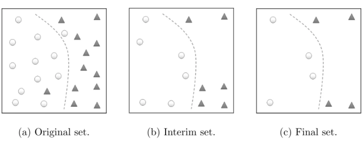
(a) Original set. (b) Interim set. (c) Final set.
Figure 2.1: An example of instance selection performed on a data set with two classes.
instances within the data set that can be used. The focus with instance se-lection is to rid the data set of outlier (which are usually detrimental to the quality of the model being built), superfluous and noisy instances. Instance selection can either start with an empty set and continuously add instances from the data set till it satisfies the objective of finding the minimum repre-sentative set, or start with the full set of instances in the data set and whittle it down to the most representative instances. Another technique that can be deployed is to replace a cluster of instances with a representative (sometimes also known as a prototype instance), which may or may not be a natural instance from the original data set. An example of a how an instance se-lection might proceed to achieve data reduction can be seen in Figure 2.1. Research in instance selection stretches as far back as the 1970’s with the advent of Wilson editing, and a survey of such algorithms is presented in the next chapter.
2.3
Classification
Classification is a data mining and machine learning field that focuses on building models that are capable of predicting the class of a given case. In particular, classifier models attempt to predict the categorical label or class of the case being studied. Given a set of labeled instances, a classification algorithm will try to capture the mapping between the attributes of the instances within the set and their respective class. Once this mapping has been captured it is used to build a model, which can take the form of a set of rules; a decision tree or a statistical model among others, which in turn is then used to predict the class of unforeseen instances. The set of instances used to build the model is usually known as a training set. Since the training set is labeled, i.e. the class of each instance is known beforehand, classification is considered to be a form of supervised learning. This is in contrast to other data mining schemes that build models from instances where no known class is present a priori, such as clustering. The effectiveness of a classifier is evaluated using a data set different from the training set, known as the testing test, and the performance of the classifier can be gauged using a number of metrics. The most common metric used for gauging classifier performance is accuracy, and it is simply the number of instances from the testing set that were classified correctly out of the total number of instances in the testing set. Over the next few subsections, we will examine three of the most common classification algorithms. For a broader coverage of classifiers, the reader is referred to [9], [19], [34].
2.3.1
k
-Nearest Neighbor
First developed in the 1950’s, the k-Nearest Neighbor classifier is considered
to be of the earliest classification algorithms. Based on learning by
compar-ison, a k-Nearest Neighbor Classifier will attempt to classify a new instance
based on the nearest representative(s) in a set of maintained instances. Each
instance of the maintained set will haven attributes and a class label. Given
a new instance to classify, the classifier will go over its set of maintained
instances, also known as the training set, and find the k-nearest neighbors.
The proximity between instances is defined by a distance function which measures the distance between two instances by aggregating the differences
between each of then attributes for the two instances being compared. Once
located, the k-nearest neighbors then vote on the class of the new instance
by counting the number of instances per class. The class with the majority count then gets assigned to the new instance.
dist(X1,X2) = v u u t n X i=1 (x1i−x2i) 2 (2.15)
An example of a distance function that is commonly used with the k
-Nearest Neighbor classifier is the Euclidean distance, seen in Equation 2.15. Handling numerical attributes is straight forward, as the difference for each positional pair of numerical attributes is measured, squared, aggregated and the square root of the sum is returned. Before applying the distance measure, numerical attributes are usually normalized so as not to allow the numerical range of the attribute to skew the measure. For categorical attributes, the difference is considered to be one if their values do not match, and zero otherwise. The rest of the equation would apply without modification.
In the original version of the classifier, the distance measure is applied to the attributes of the instance without weighing. This made the classifier susceptible to noisy or irrelevant attributes. To remedy this, extensions were introduced that allowed the weighing of the attributes within the distance function, as well as the cleansing of noisy data.
2.3.2
C4.5
Developed by J. Ross Quinlan [5] as an extension to an earlier algorithm, the C4.5 is a greedy tree induction algorithm that recursively divides the training set into smaller and smaller sections, where each section is dominated by a particular class. Moving down the tree, each node leads to its children based on value ranges of one particular attribute. The general workings of a typical decision tree induction algorithm can be seen in Algorithm 2.
The algorithm starts by creating the root node, which starts with the entire training set of tuples and a list of attributes. It then checks to see if all the tuples belong to the same class or if the attributes list is empty. If that is the case then the node is assigned the majority class within the tuples and is returned. Next, we get the splitting criteria through the use of an attribute selection function. The attribute selection function inspects a collection of tuples, along with a list of attributes, and decides on the best attribute to split on along with the value ranges to use per branch. We then update the attribute list based on the attribute that was selected for the splitting. For each of the branches included in the splitting criteria we either add a leaf node containing the majority class of the current node if the branch being considered has no tuples or add an entire sub-tree based on the remaining
Algorithm 2 Decision Tree Induction Algorithm
1: procedure GetTree(D, attributes list)
2: N ← new node
3: if attributes list=φ or class(∀x∈D) = C then 4: N.Class← GetMajorityClass(D)
5: return N
6: end if
7: split criterion← Attribute Selection(D, attributes list)
8: update attributes list
9: for j ∈split criterion do
10: Dj ← Split(D, j)
11: if Djis empty then
12: leaf ← GetMajorityClass(D)
13: N.Children←N.Children∪leaf
14: else
15: N.Children←N.Children∪GetT ree(Dj, attributes list)
16: end if
17: end for
18: return N
attributes and tuples associated with the branch being considered.
As mentioned earlier, the attribute selection function decides on the next attribute to split on. The first function used by Quinlan is known as Infor-mation Gain, and is defined as:
Gain(A) = Inf o(D)−Inf oA(D) (2.16) where Inf o(D) =− m X i=1 pilog2(pi) (2.17) Inf oA(D) v X j=1 |Dj| |D| ×Inf o(Dj) (2.18)
Equation 2.16 measures the gain in purity if an attribute A is used for
the split. Purity in this sense is attempting to have a set where all the tuples share the same class, or have this set as homogeneous as possible. Equation
2.16 measures this gain by seeing how entropy in the original setDis reduced
by splitting on attribute A. Equation 2.17 attempts to measure the amount
of information required to classify a tuple in D encoded as bits (thus the
use of log2 in the function). This information is measured by averaging the
probabilities of an arbitrary tuple belonging to a class Ci. Once the entropy
associated with the original tuple setD, we then test the amount of entropy
that would removed by an attribute A using Equation 2.18. This function
does the same as the previous one but on a smaller scale: on the scale of the tuple set that would result if we split on a value of the attribute at hand. To split using Information Gain, we simply select the attribute that returns the maximum gain. (To see Information Gain in action, the reader is referred to [9])
Using information gain had an issue that it was biased towards selecting the attributes that had a large number of unique values such as a row iden-tifier which would not have value in classification. To remedy this, Quinlan introduced Gain Ratio, a successor of Information Gain and is the basis of the C4.5 extension. GainRatio(A) = Gain(A) SplitInf o(A) (2.19) where SplitInf oA(D) = − v X j=1 |Dj| |D| ×log2( |Dj| |D|) (2.20)
Note that Equation 2.20 takes into account the number of tuples in the resultant set post split. By doing so, Gain Ratio favors those splits that result in larger sets versus those which result in smaller sets, thus alleviating the bias towards attributes with a large number of unique values.
2.3.3
Naive Bayes
The Naive Bayes classifier is a statistical classifer based on Bayes’ Theorem. Although a relatively simple classifier, the Naive Bayes classifier has shown to be competitive with some of the more sophisticated classifiers such as decision tree induction and some forms of neural network classifiers. Over the next few paragraphs, we will look into the basics of Bayes Theorem and how it was used to form the classifier.
Bayes Theorem
Bayes Theorem was developed in the 18th century by one Thomas Bayes, a
data described by n attributes. In the context of the theorem, X would be
considered ”evidence” of a fact. Let H be a hypothesis. In the context of
classification, such a hypothesis could be thatX belongs to a specific classC.
In order to arrive at a classification, our aim would be to find out P(H|X),
i.e. that probability of X belonging to a specific class C given the values of
attributes inX.
P(H|X) is known as a posteriori probability ofHbeing conditioned onX.
Suppose for example thatX represents a loan application with two attributes:
applicant employment status and applicant yearly income. Now suppose that
the values of these attributes were ”Employed” and ”≥ 100,000”. For our
hypothesis, suppose that it would be whether the loan application is rejected
or approved. P(H|X) in this case would be whether a loan application
is approved or rejected knowing that the applicant’s employment status is
”Employed” and that his yearly income is ”≥100,000”.
P(H) orP(X) are known as a priori probability since their measurement
is unconditional on the presence of other facts. This probability can be easily calculated using basic information that is supplied from the data set being analyzed.
Since our focus here is classificaiton, our aim is to calculate P(H|X) for
the various classes present with theX at hand. Bayes’ Theorem allows us to
estimate this probability using Equation 2.21.
P(H|X) = P(X |H)P(H)
Classification Algorithm
Now that we have seen Bayes’ Theorem, let us see how it used to classify tuples or instances.
1. Let T be a set of training data. Each tuple X in the training data is
made up of n attributes.
2. Let there be m classes in T, C1,C2, ...,Cm. The aim here would be to
get the maximizeP(Ci|X). This can be calculated using Equation 2.21
3. Since the denominator in the Bayes equation (P(X)) is constant, we
only need to worry about maximizing the numerator, i.e. P(X |Ci)P(Ci).
4. Using the assumption of conditional independence, we can estimate
P(X |Ci) with P(X |Ci) = n Y k=1 P(xk|Ci) (2.22)
where k represents the positional index of the attributes in X. If the
attribute being handled is categorical, then the estimation of probabil-ity is a simple matter of counting occurrences and dividing by the total
number of instances in Ci. If the attribute is numerical however, then
we can safely assume that it follows a Gaussian distribution within the data and the process of calculating its probability would involve cal-culating the mean and variance for that attribute and then using the Gaussian distribution function to estimate the probability.
5. After calculating the probabilities for a given X to belong to each of
Related Work
In this chapter, we will look into previous work done with ACO and Data Reduction that is relevant to the research proposed in this article.
3.1
Ant Colony Optimization
Classically applied to combinatorial optimization problems, ACO has been extended to tackle a number of other classes of problems, including ordering problems, assignment problems, subset problems and grouping problems. Since the research introduced in this thesis is related to classification, I will focus on some of the applications of ACO in that field and would direct the reader to [17] for a survey of ACO’s application in the aforementioned ones. Ant-Miner [13] is the first ant-based classification algorithm, which aims to build a list of classification rules from a training data set that can success-fully be used to classify instances in an unforeseen data set. A classification rule takes the form of:
where term refers to an assignment of a value to one attribute from the data set. Before the ants can start building these rules, the search space must first be converted into a construction graph. The nodes in the construction graph in Ant-Miner are all the possible terms that can be extracted from the data set, i.e all the possible value assignments that can be performed to the attributes in the data set. These nodes are fully connected to each other. To construct a solution, an ant will select one term from the set of nodes pertaining to one particular attribute before moving on to the next. Once the ant has selected a term per each attribute in the data set, then it has completed building the antecedent part of the classification rule. To get the consequent, the ant will get the majority vote for class on all the instances that this rule applies to. After the rule is constructed, it will go through a pruning phase that considers the impact of removing any of the terms in the antecedent on the rule’s quality. If a term’s absence from the antecedent does not negatively impact the rule’s quality, then it is removed. The ants in Ant-Miner iteratively try to arrive at new rules, and only the best rule per iteration is kept. A rule’s quality is judged based on its classification effectiveness over the instances that it covers. Once a rule is accepted, the instances covered by that rule are removed from the data set and the ants will try to arrive at new rules from the remaining instances till the number of uncovered instances falls under a prespecified threshold. As with any other ACO-based algorithm, the ants are biased to selecting one node over the other based on the heuristic information and pheromone levels associated with that node. The heuristic information used here is information entropy
information provided by a given attribute assignment or term. Terms with a high level of entropy, thus costing more to describe, are disliked and the ants would be biased against selecting them. As for pheromone updates, only the nodes associated with the last added rule have their pheromones incremented, while all other nodes have their pheromone levels decreased based on a predetermined evaporation schedule.
Since its introduction, a lot of extensions have been proposed for Ant-Miner. These extensions either aimed to address limitations in the original algorithm or improved the quality and precision of the rules that were pro-duced by it, and include the following examples. The cAnt-Miner [26], [28] extension allows Ant-Miner to handle attributes with continuous values, a capability that was missing from the original design. The use of multiple pheromone types [33], [39], [41], one per each class in the data set being pro-cessed, resulted in improvements in the quality of the rules produced as well as their simplicity. Freitas and Chan [20] have introduced an improved rule pruning procedure that resulted in shorter rules, while improving the com-putational time used while handing large data sets. Liu et al.[12] proposed an improved function for calculating the heuristic value of the terms in the construction graph, thus improving the quality of the rules produced by the algorithm.
Boryczka and Kozak [29], [35] were able to use ACO to build classifiers
based on decision trees. The authors use the splitting rule from CART
(Classification and Regression Trees) to build a heuristic function which they use in their new algorithm, dubbed ACDT. This function assigns higher heuristic value to attributes that result in splits with the highest degree of
homogeneity in the descendant nodes. ACDT was compared with CART and Ant-Miner and has shown to produce favorable results.
Salama et al. [42], [43], [45] have adapted the ACO meta-heuristic to build Bayesian Network based classifier. The ABC-Miner algorithm attempts to build a Bayesian Augmented Naive-Bayes (BAN) classifier for the entire data set. Empirical results show that ABC-Miner performed competitively to state of the art algorithms that produced a similar classifier. Another approach for building for building Bayesian Network based classifiers is to build one network per class in the data set, and was also explored by the authors of Miner. This approach was tested against the original ABC-Miner algorithm, as well as start of the art algorithms, and has shown to produce superior classification results in most cases.
More recently, ACO has been applied to the field of neural network based classifiers. Liu et al. [22] introduced a hybrid ACO algorithm that uses BP to optimize the weights on links between neurons in a feed forward neural
network. The ACOR algorithm [27] (which performs continuous
optimiza-tion) was adapted by Socha and Blum to train neural networks as classifiers [18], [24]. Finally, Abdelbar and Salama introduced ANN-Miner [44], which uses ACO to build multi-layered feed forward neural networks for use as classifiers.
3.2
Data Reduction
One of the earliest algorithms for data reduction is Wilson editing [1], also known as Editing Nearest Neighbor. This algorithm attempts reduction by going through the instances and removing those that are incorrectly classified
by their nearest neighbors, typically considering the three closest neighbors. This has the effect of removing noisy instances that lie within the body of homogeneous zones of a particular class, as well as smoothing the boundaries between zones of different classes. Two known extensions of Wilson editing
are Repeated Edited Nearest Neighbor and All k-NN [2]. In RENN,
Wil-son editing is performed iteratively until no more instances can be removed
from the data set. All k-NN is similar to RNN, but increasedk (the number
of nearest neighbors to consider) with each iteration. Both extensions pro-vided higher accuracies than Wilson editing when paired with instance based classifiers.
The IB family of algorithms are a group of incremental lazy learners introduced by Aha et al in 1991 [3]. Two of these algorithms performed reduction by means of instance selection, and therefore are of interest as they fall in-line with this proposal’s main context. With IB2, a new case is added to the set of maintained cases by the classifier if and only if it cannot be correctly classified by the set already maintained. At the end of the algorithm, the set that is used by the classifier then becomes our reduced set. This makes IB2 susceptible to noisy instances, as they will always be misclassified and thus added to the set of maintained cases by the classifier. In an attempt to remedy the problem of noisy instances, IB3 enforces a policy that removes instances from the maintained set if they contribute negatively to the classification. This is done by keeping track of how well instances in the maintained set classify instances in the training set. If that classification has a statistically significant negative record, then the instance that produced that record is removed from the set of maintained instances. IB3 has shown
to have a higher accuracy than IB2 when tested in application and since both IB2 and IB3 algorithms are incremental in nature, they are highly efficient when compared to other reduction algorithms.
Wilson et al introduced the DROP family of reduction algorithms in [10]. DROP 1 performs reduction by considering whether removing an instance would result in a misclassification of its neighbors. If that is not the case, the instance is removed. The algorithms starts with the entire training set, and for each instance in that set, it gets its nearest neighbors. The current instance is added to each of the neighbors associates list, those instances where the current instance can be found as a neighbor. It then considers the following question using each instances and its associates: if the current instance is removed from the neighborhood of each of its associates, would that result in a misclassification, or would the associates be classified cor-rectly without the influence of the current instance? If the removal of the instance at hand results in a misclassification, then it is removed, otherwise it is kept. The algorithm does this iteratively and the data set that remains after this whittling is then the reduced data set. DROP 1 attempts to remove noisy instances, since they will always cause a misclassification amongst their neighbors. DROP 1 also has a bias to remove instances that are in the center of class ”zones” as opposed to ones near the boundary, since these instances are superfluous and the membership of any newly encountered instances to the class zone can easily be inferred from the boundary instances. How-ever, in the process of removing instances, DROP 1 may resolve to remove a lot of instances around a noisy instance(s) that lies within the center of a homogeneous region of a class before the noisy instances themselves are
removed. DROP2 was designed with a measure that addresses this issue. DROP 2 differs from DROP 1 in that during iterations, it will consider the effect of leaving a considered instance on the misclassification of deleted in-stances in pervious iterations as well as those who remain. DROP 2 also adds an ordering to the process of removing instances. At the beginning of each iteration it would sort the instances still being considered for reduction by distance from their respective nearest enemy: an instance of a different class. Instances are then considered for removal starting with those furthest away from their enemies. DROP 3 adds preprocessing stage whereby Wilson editing is performed on the data set before the algorithm proceeds. Since at times this has shown be too aggressive, and in effect filtering out the entire data set, DROP 4 adds a constraint to the preprocessing phase: An instance promoted for removal by Wilson editing is only removed if doing so would not cause a misclassification with its associates. Finally, DROP 5 differs from DROP 2 in that it considers instances for removal in the reverse of the order used in DROP 2. This means that instances that are closer to their enemies are considered before those further away. This has the effect of smoothing the class zone boundaries and removing central points more efficiently than DROP 2.
Iterative Case Filtering, or ICF, is an algorithm devised by Mellish et al [11] that achieves reduction over two phases. The first phase of the algorithm performs regular Wilson editing, with a neighborhood size of 3 typically. The second phase then builds two sets for each instance that still remains: a reachable set and a coverage set. The reachable set are those instances that include the current instance in their neighborhoods. The coverage set are
those instances that have the current instance as a neighbor. In essence, the reachable set are those instances that influence the classification of the cur-rent instance, and the coverage set are those whose classification is influenced by the current instance. After having built those sets, the algorithm then removes those instances who have a reachable set larger than that of their coverage set, for those instances are considered superfluous and their removal would not affect the general accuracy of a model built on the remaining in-stances. The ICF algorithm has proven to be an efficient reduction algorithm when tested against a wide panel of data sets from UCI Machine Learning repository.
The ADR-Miner Algorithm
As alluded to earlier, the ADR-Miner adapts an ACO algorithm to perform data reduction with an emphasis on improving a classifier’s predictive effec-tiveness. In particular, given a training set, a testing set and a classification algorithm, we want to see if we can achieve more accurate predictions if the classifier is constructed using a reduced set then tested, as opposed to being constructed using the raw training set.
Adapting the ACO algorithm to perform data reduction involves a num-ber of steps:
1. Translating the problem into a search space that is traversable by the ants, also known as a construction graph.
2. Defining the overall meta-heuristic that will be used to direct the ants as they search the problem space.
3. Defining how an ant constructs a candidate solution (i.e., a reduced set) while traversing the construction graph.
4. Defining the mechanics of evaluating the quality of such solutions and updating the pheromone trails.
Over the next few sections, we will delve into the details associated with these steps and in effect describe how we can adapt ACO to perform data reduction via instance selection.
4.1
The Construction Graph
At the core of the ACO algorithm is the construction graph. This is a graph of decision components that when a subset is chosen from by an ant forms a solution to the problem being solved. Our main concern when tackling a problem is how to translate the related search into a graph of decision com-ponents with the stipulation that the graph contains subsets of the decision components that form valid solutions to the problem being solved. Take for example the traveling salesman problem, one of the first to be tackled by ACO. In the traveling salesman problem, we are given a set of cities and distances between them and asked to find the shortest route that visits all the cities exactly once and return to the origin city. Translating such a prob-lem into a construction graph would first lead us to building a graph where the nodes represent the cities and vertices between the nodes would repre-sent the distances among them. The nodes form decision components as at each node, an ant would have to ”decide” which node to visit next whilst maintaining the process of building a valid solution: not to revisit any cities already visited. From this graph of cities and distances, an ant could start at one node and iteratively decide which city to visit next till it returns to origin. The graph in its current form can thus be considered a construction
Figure 4.1: The ADR-Miner Construction Graph
graph as it could possibly contain one or more valid routes connecting all the cities. This graph was coined a ”construction” graph since the ants traverse it one node after the next, iteratively deciding which node to visit next while ”constructing” a solution.
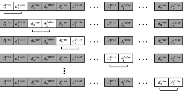
In our case, we are attempting to perform data reduction via instance
selection. Starting with a set of instancesI, we want to arrive at a subsetR ⊆
I that produces the best possible classifier effectiveness. Essentially, we have
to decide which instances fromI are to be included inR, and that translates
into each instance having two decision components within the graph: dtrue
i
whose selection would imply the inclusion of the i-th instance in I, and
df alsei whose selection would imply the exclusion of the i-th instance from I.
Selection betweendtrue
i andd f alse
i for the same value ofiis mutually exclusive,
and an ant constructing a solution cannot include both in its selection. The decision components of the graph conceptually take the form of a two
dimensional array, with a length of|I|and a depth of 2, signifying the choice
between inclusion and exclusion. A visual representation of the construction graph can be seen here 4.1. A valid candidate solution can be built from this construction graph by starting at the first node of the array, selecting either the inclusion or exclusion nodes from the second dimension and then moving onto the next node till the entire array is parsed.
4.2
The ADR-Miner Overall Algorithm
The overall procedure for ADR-Miner can be seen in Algorithm 3 We begin by initializing the pheromones on all the decision components to the value of 1 (line 4). This includes both the components for inclusion and exclusion for
all instances in the data set to be reduced (i.e., the current trainingset).
We then enter arepeat−until loop (lines 5 to 21) that is terminated when
either of the following criteria are reached: we exhaustmax iterations
num-ber of iterations, or the colony has converged on a solution and no visible
improvement has been observed overconv iterationsnumber of iterations,
wheremax iterations and conv iterationsare external parameters.
Within each iteration t of this outer loop, each anta in the colony
con-structs a candidate solution Ra (line 7), that is, a reduced set of instances.
After a candidate solution is produced, a classification model Ma is
con-structed using the reduced set Ra and an input classification algorithm g
(line 8). The quality of model Ma is evaluated (line 9), and if it is higher
than that achieved by other ants in the current iteration t, it supplants an
iteration best solution Rtbest (lines 10 to 13).
After all the ants in the colony complete the building of their solutions, the best ant in the iteration is allowed to update the pheromone trails based onRtbest. This complies with the pheromone update strategy of theMAX
-MIN Ant System [6], on which this algorithm is based. The iteration best
solution Rtbest will supplant the best-so-far solution Rbsf if it is better in
quality (lines 16 to 20). This process is repeated until the main loop exits,
at which point, the best-so-far solution,Rbsf, observed over the course of the
Algorithm 3 Pseudo-code of ADR-Miner.
1: g ←classification algorithm
2: I ← training set
3: InitializeP heromones()
4: repeat
5: for a ← 1 to colony size do
6: Ra ← anta.CreateSolution(I) 7: Ma ← ConstructM odel(g, Ra) 8: Qa ← EvaluateM odelQuality(Ma) 9: if Qa> Qtbest then 10: Qtbest ←Qa 11: Rtbest ←Ra 12: end if 13: end for
14: U pdateP heromones(Rtbest)
15: if Qtbest > Qbsf then
16: Qbsf ←Qbest
17: Rbsf ←Rtbest
18: t ←t+ 1
19: end if
20: until t =max iterations or Convergence(conv iterations)
So far, the ADR-Miner algorithm uses a single classification alg