Optimization Problems
Michel X. Goemans
1and Francisco Unda
21 MIT, Cambridge, MA, USA
2 MIT, Cambridge, MA, USA
Abstract
We consider incremental combinatorial optimization problems, in which a solution is constructed incrementally over time, and the goal is to optimize not the value of the final solution but the average value over all timesteps. We consider a natural algorithm of moving towards a global optimum solution as quickly as possible. We show that this algorithm provides an approximation guarantee of (9 +√21)/15 > 0.9 for a large class of incremental combinatorial optimization problems defined axiomatically, which includes (bipartite and non-bipartite) matchings, matroid intersections, and stable sets in claw-free graphs. Furthermore, our analysis is tight.
1998 ACM Subject Classification F.2.2 Nonnumerical Algorithms and Problems, G.1.6 Optim-ization, G.2. Discrete Mathematics
Keywords and phrases Approximation algorithm, matching, incremental problems, matroid in-tersection, integral polytopes, stable sets
Digital Object Identifier 10.4230/LIPIcs.APPROX/RANDOM.2017.6
1
Introduction
Usually, in the context of combinatorial optimization, a single solution is sought which optimizes a given objective function. This for example could be designing (or upgrading) a network satisfying certain properties. But the solution might be large, and implementing it may mean proceeding in steps. As the adage says “Rome wasn’t built in a day”. Therefore it becomes important to consider not just the value of the (final) solution, but also the values at intermediate steps. Such incremental models have gained popularity in the last years [7, 1, 9], because of their practical applications to network design problems, disaster recovery, and planning.
As a first approximation to this extra level of complexity, we consider the setting in which we want to evaluate our solution at each time step, and would like to maximize the sum of the values of the intermediate solutions. To formalize this, consider a finite ground set Eof
qelements, together with a valuationv: 2E→
Z+. The valuation function measures some quantity of interest over a subset ofE, for example, the size of a maximum matching, the maximum value of an independent set in a matroid, or a maximum flow. Our goal is to find a permutationσ:E→ {1, . . . ,|E|}that maximizes
f(σ) =
q X
i=0
v({e∈E:σ(e)≤i}). (1)
This is a very general class of problems, which also includes for example scheduling problems, production planning problems and routing problems; such problems typically involve finding a permutation of tasks to perform.
© Michel X. Goemans and Francisco Unda; licensed under Creative Commons License CC-BY
Approximation, Randomization, and Combinatorial Optimization. Algorithms and Techniques (APPROX/RAN-DOM 2017).
Even for simple, polynomially computable valuationsv, the problem of finding the best
σmight be NP-hard. This applies for example to the situation in whichE corresponds to some of the edges of a directed or undirected graphG= (V, E0∪E) with capacities on its edges, andv(F) represents the maximum flow value fromstot(wheres, t∈V) in the graph (V, E0∪F). The NP-hardness of this incremental problem was shown by Nurre and Sharkey
[9], see also Kalinowski et al. [7].
On the tractable side, the incremental problem (1) can be solved efficiently if v(F) represents the weight of a maximum-weight independent subset ofF in a matroidM with ground setE. Indeed, an optimum permutation can be obtained from a maximum-weight independent setB for the entire ground setE in the following way. First, orderB in order of non-increasing weight followed by all elements ofE\B in an arbitrary order. In the case of the incremental spanning tree problem, this was also derived in [6].
In this paper, we consider a class of valuationsv which arise naturally from unweighted combinatorial optimization problems, and for which we are able to provide a worst-case analysis of a greedy-like algorithm. This class of valuations is defined axiomatically. First, we require thatvtakes nonnegative integer values,
(A1): ∀F ⊆E :v(F)∈N
and is monotonically non-decreasing and can only increase by at most 1 when an element is added:
(A2): ∀A⊂E,∀e∈E\A:v(A)≤v(A∪ {e})≤v(A) + 1.
Additionally, we assume that for any kwithv(∅) = minFv(F)≤k≤maxFv(F) =v(E),
there exists a set of cardinality at mostkachieving the valuek:
(A3): For allk:v(∅)≤k≤v(E),∃A⊆E:|A| ≤k andv(A) =k.
Consider, for example, an independence systemI onE0∪E, i.e.I ⊆2E0∪E andI is closed under taking subsets. Then if we definev(F) forF ⊆E as the cardinality of the largest independent subset ofE0∪F, we can easily see thatv(·) satisfies (A1), (A2) and (A3). This generalizes the matroid setting mentioned previously.
We further assume one additional key property, that v satisfies the followingdiscrete convexity property:
(A4) Discrete Convexity: ∀A, C ⊆E withv(C)−v(A)>1,∃B : v(B) = v(A) + 1 and
|B| − |A| ≤ v(|C|−|A|C)−v(A).Furthermore ifA⊂C thenA⊂B⊂C.
This discrete convexity is not satisfied by all independence systems. However, we show in Section 2 that if a certain family of polyhedra is integral then the discrete convexity property is satisfied.
ITheorem 1. LetI ⊆2E0∪E be any independence system. LetP(I)⊆
RE0∪Ebe the convex
hull of incidence vectors of all independent sets inI. If for every integerk,
P(I)∩ ( x| X e∈E0∪E xe=k )
is integral then(A4) holds forv: 2E→Z+ defined as v(F) = max{|I| |I∈ I, I⊂E0∪F}. In Section 2, we show that this holds for example whenI corresponds to the matchings in a (not necessarily bipartite) graph, or to the independent sets common to two matroids, or to the (independent or) stable sets in a claw-free graph. This last example, although more esoteric, is interesting as a complete description ofP(I) by linear inequalities is unknown but we can nevertheless rely on the above theorem. The incremental valuation problem in the case ofbipartite matchings was already considered in [7], where the authors propose
Algorithm 1:Quickest-To-Ultimate for Incremental Valuation
Input :A valuation functionv as above.
Output :A permutationσofE
1 ComputeO⊆E of minimum cardinality such thatv(O) =v(E); 2 SetF =∅;
3 fori= 1tov(E)−v(∅)do
4 ComputeS⊂O\F such thatv(F∪S)≥v(∅) +iand|S|is minimum; 5 SetF =F∪S;
6 end
7 Output σconsistent with how elements were added to S;
several approximation algorithms, the best achieving an approximation ratio of 3/4. Other problems falling under the framework discussed here were not considered before.
For any valuation satisfying (A1)−(A4), we provide an approximation algorithm for the incremental valuation problem. For an efficient implementation, we assume that we can compute efficiently (or have oracle access to) the valuation v(·) and we can also find efficiently a minimum cardinality setO withv(O) =v(E). Our algorithm first computes a smallest setO ⊆E achievingv(O) =v(E), and then starting fromS=∅ with valuev(∅), repeatedly and greedily adds a smallest subset ofOto increasev(S) by 1 until all elements of
Ohave been added and then finishes the ordering with the elements ofE\O. This algorithm is formally described in Section 3 and in Algorithm 1. In Section 3, we present a worst-case analysis of this algorithm:
ITheorem 2. For any valuation satisfying(A1)−(A4), Algorithm 1 (Quickest-to-Ultimate) is aγ-approximation for the incremental valuation problem, where
γ= 9 +
√
21
15 >0.9055.
The proof of this result is given in Section 4. We also show that the bound ofγis tight in the sense that there are instances of the valuation problem in which the algorithm cannot do better.
2
Problems in this Framework
2.1
Maximum matchings
One of the basic problems that falls in this framework is theIncremental Matching Problem. Given a graphG= (V, E0∪E), whereE0 denotes the edges already present at the start, we would like to find an ordering of the edges ofE so as to maximize the average size of the maximum matching inE0 union the edges already selected. This corresponds to the valuation withv(F) =µ(E0∪F) whereµ(A) equals the size of the maximum matching in the graph (V, A). The bipartite version of this problem is considered in [7], and two different greedy approximation algorithms are presented. The first one,Quickest-Increment, is a locally greedy algorithm that seeks to minimize the number of edges needed to increase the size of the matching by one, until we reach a maximum matching of the entire graph. Kalinovski et al. [7] prove an approximation guarantee of 23 for this algorithm. Their second algorithm,Quickest-to-Ultimate, is globally greedy, in the sense that it first computes a maximum matching of the entireG, and then only adds edges from this matching, in a locally greedy fashion. For this algorithm, [7] prove an approximation bound of 34. In this
paper, we generalize this algorithm to a larger class of incremental problems and improve the guarantee to 0.9055· · ·.
This matching problem, even in the non-bipartite case, fits in the framework discussed here. One can show that this valuationv(F) =µ(E0∪F) satisfies the discrete convexity property (A4), by considering maximum matchings inA andC, and their symmetric difference and carefully arguing about it. Although this is possible, this does not generalize easily to other problems.
Discrete convexity, however, is easier to argue polyhedrally as we show next.
2.2
Polyhedral characterization for discrete convexity
LetI ⊆2E0∪Ebe any independence system, and letv(F) = max{|I|:I∈ IandI⊆E
0∪F}. LetP= conv{χ(I) :I∈ I}be the convex hull of all independent sets, and as we will see, we do not necessarily need to know a complete description ofP in terms of linear inequalities. We will show Theorem 1 that discrete convexity (A4) holds if, for any integerk,
P∩ {x:x(E∪E0) =k} is integral.
Proof of Theorem 1. For A(resp. C), letIA (resp. IC) be a maximum independent subset of E0∪A (resp. E0∪C). So, v(A) = |IA| andv(C) = |IC|. Let ` = |IC| − |IA|. Now
consider y = 1`χ(IC) + (1−1
`)χ(IA). By convexityy ∈P and by construction, we have y(E∪E0) =|IA|+ 1. Thus,y∈P∩ {x:x(E∪E0) =|IA|+ 1}, and by integrality of this
polytope, we have that there existsx=χ(S)∈P∩ {x:x(E∪E0) =|IA|+ 1}with
|S∩E| = min{x(E) :x∈P∩x(E∪E0) =|IA|+ 1} ≤ y(E) =1 `|IC∩E|+ (1− 1 `)|IA∩E| ≤ 1 `|C|+ (1− 1 `)|A|=|A|+ |C| − |A| v(C)−v(A).
ThusB=S∩Esatisfies the first part of the claim in Theorem 1. Now consider the case in whichA⊆C. Proceeding as before, we get
y∈P∩ {x:x(E∪E0) =|IA|+ 1} ∩ {x:xe= 0∀e∈E\C},
and this is again an integral polytope since it is the face of an integral polytope. Now minimizingx(E\A) over
P∩ {x:x(E∪E0) =|IA|+ 1} ∩ {x:xe= 0∀e∈E\C},
we getx=χ(T)∈P∩ {x:x(E∪E0) =|IA|+ 1}withT ⊆E0∪C and
|T∩(E\A)| ≤y(E\A) = 1
`|IC∩(E\A)| ≤
|C| − |A|
v(C)−v(A). This means thatB =A∪(T∩E) is such thatA⊆B⊆C,
|B| ≤ |A|+ |C| − |A|
v(C)−v(A)
andv(B)≥v(T) =|IA|+ 1. Thus eitherv(B) =|IA|+ 1, or we can eliminate one by one elements ofB\A as long asv(·) is not equal tov(A) + 1. Eventually, we find a set with the
2.3
Maximum stable set in claw-free graphs
A graph G= (V, E) is claw-free if it does not includeK1,3 (the star on 4 vertices) as an induced subgraph. The line graph of any graph is claw-free, but the converse is not true as there exist claw-free graphs which are not line graphs. Minty [8] and Sbihi [10] have shown that the maximum stable (or independent) set in a claw-free graph is polynomially solvable. When the claw-free graph is a line graph, this extends Edmonds’ algorithm [4, 3] for maximum matching, as the maximum matching problem in a graph is equivalent to the maximum stable set problem in its line graph.
By taking the line graph, we can extend the incremental matching problem to an incremental stable set problem in a claw-free graph G= (V, E) in which we are given an initial vertex set V0 and our task is to choose an ordering of the remaining vertices in
V \V0 so to maximize the average size of a maximum stable set in the corresponding prefix. Thus, herev(F) denotes the size of the largest stable set inG[V0∪F]. As said before, if the claw-free graph is not a line graph, this is a strictly more general problem than the incremental matching problem.
A complete description of the stable set polytopeP for claw-free graphs is still unknown (see, eg, section 69.4a in Schrijver [11]), but we can nevertheless use Theorem 1 to show that (A4) holds (the other conditions (A1), (A2) and (A3) obviously hold).
ITheorem 3. LetP be the stable set polytope of a claw-free graph G= (V, E). Then for any integerk, we have that
P∩ ( x∈RV | X v∈V xv =k ) is integral.
Proof. We exploit the known adjacency properties of the stable set polytope (of any graph). Chvátal [2] has shown that two stable setsS1 andS2 inGare adjacent vertices in the stable set polytope if and only if their symmetric differenceS14S2 induces a connected subgraph ofG. When the graph is claw-free, this connected subgraphG[S14S2] must be a path, and therefore this means that−1≤ |S1| − |S2| ≤1.
Consider any vertexx∗ofP∩
x∈RV |P
v∈V xv=k . x∗must lie on a face of dimension
at most 1 ofP, and therefore must be in the line segment between two adjacent vertices of
P. But since the sizes of these stable sets can differ by at most 1, we derive thatx∗ must be
a vertex ofP, and integrality follows. J
Thus our approximation algorithm result applies to the incremental maximum stable set problem in claw-free graphs.
The adjacency argument in the proof of Theorem 3 generalizes in the sense that Theorem 1 is equivalent to imposing that any pair of adjacent vertices ofP(I) differ in cardinality by at most one unit.
2.4
Matroid intersection
Another generalization of the incremental version of the bipartite matching problem is to consider the incremental version of matroid intersection. LetM1andM2be matroids defined on the same ground set, sayE0∪E, and forF ⊆E, letv(F) be the cardinality of the largest common independent set to the two matroids withinE0∪F.
For matroid intersection, we can directly use Theorem 1 to show that the discrete convexity holds. The matroid intersection polytopeP has been characterized by Edmonds [5], and the integrality ofP∩ {x|P
ixi =k} follows simply by truncating both matroids to sizek. Thus
Theorem 1 can be used to prove (A4) and Theorem 2 can be used to derive a better than 0.9-approximation algorithm for the incremental maximum matroid intersection problem.
3
Quickest-To-Ultimate for Incremental Problems
Algorithm Quickest-To-Ultimate (Q2U in short, see Algorithm 1) was introduced by Kalin-owski et al. [7] for the problem of incremental flows (defined in the introduction). The general idea behind this algorithm is to reach the maximum valuation possible in the shortest number of steps. In the setting of incremental flows, finding the smallest setOof edges whose addition gives a maximum flow is a hard problem, and they resort to a mixed integer program for findingO. In this direction it is known that the incremental flow problem is NP-hard even if the capacities are restricted to be one or three [9]. In the case of unit capacities, Q2U becomes a polynomial approximation algorithm, and in [7] it is shown that it finds a solution with at least half the value of the optimum for the incremental flow problem with unit capacities, and they also show a matching family of examples in which this approximation ratio is attained as the size of the graph grows. In the case of bipartite matchings, a further restriction of the problem, Q2U is shown to find a solution to the incremental matching problem of value at least 3/4 of the optimum, and they show an instance in which the value obtained by Q2U is 6869 of the value attained by the optimal solution. Theorem 2 and the example given in Section 3.1 below close this gap for a more general class of valuations, which includes the incremental matching problem.
We show Theorem 2, that for any valuation satisfying (A1)-(A4) the performance guarantee of the algorithm is at least 9+
√
21
15 >0.9055. The proof appears later in this section, and our analysis is tight as we show next.
3.1
Bad instance for Quickest-to-Ultimate
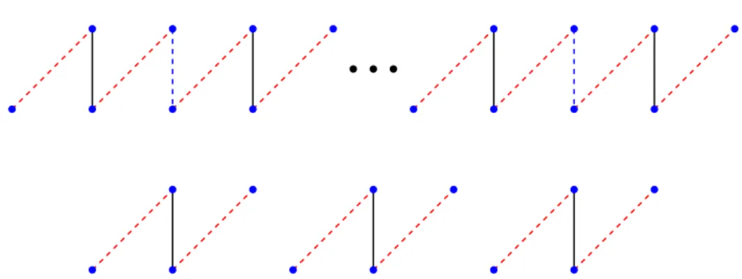
In the special case of matchings, and even bipartite matchings (or any setting which includes bipartite matchings), the analysis is tight. Consider, indeed, a graph formed byadisjoint copies of P3, a path with 3 edges, and one copy of P4b+3, a path with 4b+ 3 edges, see
Figure 1. The edges ofE0 correspond to each middle edge in the copies ofP3, and every fourth edge ofP4b+3, starting with the second one. The remaining edges are edges ofE. The
valuation is v :E →N, wherev(S) is the size of a maximum matching using edges from
E0∪S.
In this graph, we haveq:=|E|= 2a+ 3b+ 2 edges to be added, the original matching has sizem:=a+b+ 1, and it can grow byr:=a+b+ 1. The minimum number of edges we need to add to reach this maximum matching iscr:= 2a+ 2b+ 2. Quickest-to-Ultimate adds these edges in pairs that increase the matching, so it adds two edges for each increment in the maximum matching. The value it attains is thenfalg= (q+ 1)(m+r)−Pa+b+1
i=1 2i= 3a2+ 5b2+ 8ab+ 7a+ 9b+ 3. On the other hand, here is a better solution. The solution first adds theb edges ofP4b+3 that increase the maximum matching frommtom+b, then it addsa pairs of edges to increase the matching by a and then it adds 2b+ 2 edges to increase the matching by one. This gives a valuef withfopt≤f = (q+ 1)(m+r)−P
b i=1i− Pa+b i=b+1(2(i−b) +b)−(2a+b+ 2b+ 2) = 3a 2+11 2b 2+ 9ab+ 7a+17 2b+ 4. A straightforward optimization overaandb, yields that the minimum value of falg
Figure 1Solid black edges are edges ofE0 and dashed edges are the edges ofE.
go to infinity, witha=δb, withδ=
√ 21 6 − 1 2, with value of 9+√21
15 . This is the worst case for Q2U and matches the bound we prove in Theorem 2.
4
Analysis
Before diving into the analysis of Q2U, we introduce some notation and exhibit some convexity properties of various sequences associated with these incremental problems.
We denote v(∅) bym,v(E) by m+r, and|E|byq. For any permutationσofE, define
di(σ) :=|{j∈ {0, . . . , q} : v({e∈E : σ(e)≤j})≤m+i−1}|,
which is the number of elements needed for the solutionσto get to a valuationm+i. We will denote byd∗i the values ofdi(σ∗) for an optimal solutionσ∗ to (1), and bydi the values ofdi(σ) for the permutationσoutput by Q2U.
Define for eachi∈ {0, . . . , r}
ci:= min{|S| : v(S)≥m+i}.
By definition, we haveci≤di and similarly ci≤d∗i. Also by (A2) we must haveci ≥i, and by (A3),
ci≤m+i, (2)
fori∈ {0, . . . , r}.
We show that our assumptions imply that both the sequence {ci}r
i=1, and the sequence
{di}ri=1 satisfy a convexity property.
ILemma 4. The sequence {ci}r
i=1 satisfies
ci+1−ci≥ci−ci−1, 1≤i≤r−1.
Proof. To see this, apply (A4) to the respective solutionsSi−1, Si, Si+1 where
Sj= arg min
S {|S|:v(S)≥m+j}.
Note first that by (A2) we have that v(Sj) = m+j for j = i−1, i, i+ 1. This implies
v(Si+1)−v(Si−1) = 2>1, and so by (A4), there existsBsuch thatv(B) =v(Si−1)+1 =m+i
and 2(|Si| − |Si−1|)≤2(|B| − |Si−1|)≤(|Si+1| − |Si−1|). This implies Lemma 4. J The solution given by Q2U also satisfies this same convexity property.
ILemma 5. The sequence{di}r
i=1 corresponding to Q2U satisfies
di+1−di≥di−di−1, 1≤i≤r−1.
Proof. To see this, denote bySi the set computed in the inner loop of the algorithm at step
i. That isSi⊂Fr\(S1∪. . .∪Si−1) such that|Si|is minimum andv(S1∪. . .∪Si)≥m+i.
Minimality of|Si|, and property (A2) imply thatv(S1∪. . .∪Si) =m+i, and then di =
|S1∪. . .∪Si|. Now takei∈ {1, . . . , r−1}. Thenv(S1∪. . .∪Si+1)−v(S1∪. . .∪Si−1) = 2>1, and then by property (A4) there is aBsuch thatv(B) =m+iand 2(|B|−di−1)≤di+1−di−1.
Finally by minimality of|Si|we must have di ≤ |B|, which implies the claim. J We could also show that any optimum orderingσ∗ satisfies the same convexity property:
d∗i+1−d∗i ≥d∗i −d∗i−1for alli, although we will not need this. This requires the second part of (A4) which says that ifA⊆CthenB can be chosen to be sandwiched by AandC.
4.1
Local minima
We also show that the convexity property (A4) implies a relationship between local and global optima, that will be used to derive the optimal upper bound for the Quickest-To-Ultimate Algorithm 1.
ILemma 6. LetS andT be two subsets ofE, such thatv(S) =m+|S|andv(T) =m+|T|, and let S be maximal with this property, that is for any S0 ⊃S we have v(S0)< m+|S0|. Then, 2|S| ≥ |T|.
This is a generalization of the well-known result that any maximal matching is at least half the size of a maximum matching.
Proof. If|S| ≤ |T|, there is nothing to prove, so we assume that|T|>|S|. Now use (A4) with
A=S andC=S∪T. Then there is a setBwithS ⊂B ⊂S∪T such thatv(B) =v(S) + 1 and
|B| − |S| ≤ |S∪T| − |S|
v(S∪T)−v(S) ≤
|T| |T| − |S|.
On the other hand, by the maximality ofS, we must have|B| − |S| ≥2. Putting these two together yields 2≤ |T| |T| − |S|, or equivalently 2|S| ≥ |T|. J
4.2
Quickest-To-Ultimate
To analyze Quickest-To-Ultimate, we need to introduce some additional parameters related to the instance being considered. Define
p= max{|P| : P ⊂E, v(P) =m+|P|},
the maximum size of a set that, if added sequentially, increases the valuation at each step. In other words,p= max{i:ci=i}. Clearly p≤r. Also, by maximality of p, we have that
ci=i i≤p
ci≥p+ 2(i−p) i > p.
For Q2U, we are interested in the quantitys, the number of times the setS in the inner loop is a singleton. Note that by Lemma 5, thesesiterations occur at the beginning, so an equivalent way to definesis
s= max{i∈ {1, . . . , r} : di=i}.
Our objective is to relate the quantitiessandp, which will give us some control over the approximation ratiofalg/fopt. We must haves≤p, since otherwise it would contradict the maximality of p. To get a lower bound ons, define S to be the set of the firstselements added by the algorithm, and T =P ∩O, where O is the set of elements chosen by Q2U to first reach v(E) and P is a set of p elements withv(P) = m+p. Note that we have
v(S) =m+|S|andv(T) =m+|T|, andS must be maximal, by definition ofs. Then by using Lemma 6, we conclude that 2|S| ≥ |T|=|P∩O|. This implies that
q=|E| ≥ |O∪P|=|O|+|P| − |O∩P| ≥cr+p−2s. (4) And we also know that
q≥cr. (5)
Finally, we need the following inequality. Observe that all the elements that are used by the algorithm come fromO, and conversely, all the elements ofOmust be used by the algorithm to reach valuationv(E), by minimality ofcr. This means that|O|=cr=dr=Pr
i=1(di−di−1), and using the definition ofs, then cr=s+Pr
i=s+1(di−di−1), from which it follows that
cr≥2r−s. (6)
We are now ready to prove Theorem 2.
Proof of Theorem 2. For any permutationσ, we can rewritef(σ) as
f(σ) = (q+ 1)(m+r)−
r X
i=1
di(σ). (7)
In particular, for the optimum permutationσ∗ and its optimum valuefopt=f(σ∗), we have:
fopt= (q+ 1)(m+r)− r X i=1 d∗i ≤(q+ 1)(m+r)− r X i=1 ci. (8)
Using (3) and distinguishing between i≤p,p < i < r andi=r, we can write:
fopt≤(q+ 1)(m+r)−p2/2−p/2 +pr−r2+r−cr. (9)
Now, denoting the value obtained by Q2U asfalg, and using the definition of s, we have
falg= (q+ 1)(m+r)− r X i=1 di= (q+ 1)(m+r)− s−1 X i=1 i− r X i=s di. (10)
To upper bound the last term of (10), we use the following lemma, whose proof is given in the appendix.
ILemma 7. Letf : {0, . . . , a} →Nbe a discrete convex function, i.e. f(i+ 1)−f(i)≥
f(i)−f(i−1), such that f(0) = 0 and f(a) = b. Furthermore let b = ka+t, where t∈ {0, . . . , a−1}. Then, a X i=0 f(i)≤(b+ka2+t2)/2 = (a+ 1)b 2 − t(a−t) 2 .
Applying this tof(i) =ds+i−s, we obtain
falg ≥(q+ 1)(m+r)−s(s−1)/2−(r−s+ 1)s−(r−s+ 1)(cr−s)/2 +t(r−s−t)/2,
wheret=cr−smodr−s. Or after simplification:
falg ≥(q+ 1)(m+r)−rs/2−(r−s−1)cr/2 +t(r−s−t)/2. (11) We need to find the minimum value attainable byfalg/fopt≤1, which is a lower bound on the approximation ratio. We will show that this lower bound coincides with the upper bound given by the example in Section 3.1. Denote byPopt(resp. Palg) the right-hand-side
of inequality (9) (resp. (11)). To find this lower bound, we maximizePopt/Palg over all integralq, m, cr, r, p, sand tsatisfying the conditions:
1. r≥p≥s≥0 2. (5): q≥cr 3. (4): q≥cr+p−2s 4. (6): cr≥2r−s 5. m+r≥cr 6. t=cr−smodr−s.
We first show that the we can ignore all but the quadratic terms in the variablesq, m, r, p, s, t. If we double each ofq, m, cr, r, p, s, thentalso doubles by6, and all inequalities1-5are still satisfied. Furthermore, if we denotePopt0 and Palg0 the respective values of the bounds after doubling, we have Popt0 Palg0 = 4Popt−2(m+r) +p−2r+ 2cr 4Palg−2(m+r) +cr ≥ 4Popt−2(m+r) +cr 4Palg−2(m+r) +cr ≥ Popt Palg,
where in the first inequality we have used thatcr−2r+p≥cr−2r+s≥0,by4, and the second inequality follows from5.. So, for the extremum, we can assume there are no linear terms:
Popt Palg ≤
q(m+r)−p2/2 +pr−r2
q(m+r)−rs/2−(r−s)cr/2 +t(r−s−t)/2. Now, using the inequality5, we can eliminatem, and obtain
Popt Palg ≤
qcr−p2/2 +pr−r2
qcr−rs/2−(r−s)cr/2 +t(r−s−t)/2.
The remaining constraints are now1–4and6. Ifs >0, andq > cr+p−2swe can decrease
all variables by one unit, and preserve the above inequalities. In so doing, the value oftdoes not change, and both the numerator and denominator decrease by the same amount
cr+q−r−1/2≥0.
This implies we can decrease all variables by the same amount until one of two things happen. Eithers= 0, orq=cr+p−2s. In the latter case, since we also have thatq≥crby2, this
implies that 2s≤p. At this point, after eliminatingq(and replacing it bycr+p−2s), the ratio becomes: Popt Palg ≤ (cr+p−2s)cr−p 2/2 +pr−r2 (cr+p−2s)cr−rs/2−(r−s)cr/2 +t(r−s−t)/2 .
If we decrease all remaining variables by one unit, both the denominator and numerator of the above fraction decrease by
cr+p−r−2s+ 1/2≥0,
since p≥2sandcr≥r. And we can continue this process until s= 0. In both cases we obtain
Popt Palg ≤
(cr+p)cr−p2/2 +pr−r2
(cr+p)cr−rcr/2 +t(r−t)/2. (12)
And we need to maximize this over integral solutions tor≥p≥0,cr≥2randt=crmodr.
We consider two cases, depending on the value ofcr.
1. If cr= 3r+k, fork≥0, and we discard the (nonnegative) term involvingt in (12), we
obtain:
Popt Palg ≤
8r2+ 4rp−p2/2 +k(6r+p+k) 15r2/2 + 3rp+k(11r/2 +p+k).
As an upper bound, we can take the maximum of this value fork= 0 and the ratio of the terms involving k, and therefore obtain that:
Popt Palg ≤max 8r2+ 4rp−p2/2 15r2/2 + 3rp , 6r+p+k 11r/2 +p+k .
The second term on this maximum is at most 1211 <γ1 whereγis our desired bound. The first one, by setting α=r/p≥0, is equal to
8α2+ 4α−1/2 15α2/2 + 3α .
This ratio is maximized forα=58+
√
41
8 ,and it achieves a value of 112√41 + 656
99√41 + 615 < 1
γ.
2. If 2r≤cr<3r, thencr= 2r+t, and (12) becomes:
Popt Palg ≤
3r2+t2−p2/2 + 3pr+pt+ 4rt 3r2+t2/2 + 2pr+pt+ 4rt .
It is easy to see that for any constant C, and fixed values ofrand p, the set
I={t∈[0, r] : 3r
2+t2−p2/2 + 3pr+pt+ 4rt 3r2+t2/2 + 2pr+pt+ 4rt ≤C},
is a convex set, and so the maximum value of this ratio is achieved at either t= 0 or
t=r. If we sett=r, we obtain 8r2+ 4pr−p2/2
15r2/2 + 3pr < 1
Algorithm 2: Quickest-Increment for Incremental Valuation
Input :A valuation functionvas above.
Output :A permutationσofE 1 SetF =∅;
2 fori= 1 tordo
3 ComputeS⊂E\F such thatv(F∪S)≥v(∅) +iand|S|is minimum; 4 SetF =F∪S;
5 end
6 Outputσconsistent with how elements were added to S.;
as we have already verified. Ift= 0, we obtain 3r2+ 3pr−p2/2 3r2+ 2pr , which is maximized at α=r/p= 1 2+ √ 21 6 , with value 1 γ = 9 4− √ 21 4 , orγ= 9+√21 15 . J This settles the question of how well Quickest-to-Ultimate approximates the maximum incremental matching problem.
5
Upper bound for Quickest-Increment
Quickest-Increment (QI) is another algorithm suggested in [7]. The idea is to increase the size of the current solution by adding as few elements as possible. In that paper, among other results, it was shown that QI has a performance guarantee of 2/3 in the case of bipartite matchings, and also they claim a bound of 3/4 ifr≥70. It is also conjectured there that, asr→ ∞, the approximation guarantee for Quickest-Increment approaches 1. We show a family of instances that show that this is false.
Consider the instance H formed by P7, the path with seven edges, in which the only edges ofE0 are the second and the second to last. Observe that both Q2U and QI have the same performance on this small graph, and it is even optimal. In this small graph we have
q= 5,r= 2 andm= 2. There are two incomparable choices fordi. The first one, given by
Q2U, isd1 = 2 =d2. The second one is given by QI and it isd1= 1, d2= 4. They both have value 18, which is optimum.
Now consider the instanceG, which isacopies ofH. Both algorithms fail to realize the optimum. When consideringacopies, we obtainq= 5a,r= 2aandm= 2a. Algorithm Q2U returnsdi = 2i fori= 1, . . . ,2a, with a value off = (5a+ 1)(4a)−P2a
i=12i= 16a 2+ 2a. Algorithm QI returndi=ifori= 1, . . . , aanddi= 4(i−a) +afori=a+ 1, . . . ,2a, with a
value off = (5a+ 1)(4a)−Pa i=1i−
P2a
i=a+1(4i−3a) = 33a
2/2 + 3a/2.
Now suppose we use the QI strategy onk of theacopies and the Q2U strategy on the rest. Then we getdi =i for i= 1, . . . , k, di =k+ 2(i−k) fori=k+ 1, . . . ,2a−k and di= 4(i−2a+k) + 4(a−k) +kfori= 2a−k+ 1, . . . ,2a, and a value of
f = (5a+ 1)(4a)− k X i=1 i− 2a−k X i=k+1 (2(i−k) +k)− 2a X i=2a−k+1 (5(i−2a+k) + 4(a−k) +k) f = 16a2+ 2a−(3k2/2 +k/2−2ak).
Optimizing overkwe obtain that fork= 2a/3, this solution has a value off = 50a2/3 + 5a/3. So asymptotically as we takea→ ∞the approximation factor for Q2U approaches 2425 and for
QI is approaches 99
100. Note that this family of examples hasr= 2a→ ∞, and so contradicts the conjecture about QI in [7]. Note this also shows that the approximation guarantee of Q2U is bounded, even whenr→ ∞. It is possible to show a family of examples that show that whenr→ ∞, the approximation guarantee for QI approaches 78.
References
1 M. Baxter, T. Elgindy, A. T. Ernst, T. Kalinowski, and M. W. P. Savelsbergh. Incremental network design with shortest paths. European Journal of Operational Research, 242:51–62, 2015. doi:10.1016/j.ejor.2014.04.018.
2 V. Chvátal. On certain polytopes associated with graphs.Journal of Combinatorial Theory, Series B, 18:138–154, 1975. doi:10.1016/0095-8956(75)90041-6.
3 J. Edmonds. Maximum matching and a polyhedron with 0,1 vertices. Journal of Research National Bureau of Standards, Section B69, pages 125–130, 1965.doi:10.6028/jres.069B. 013.
4 J. Edmonds. Paths, trees and flowers.Canadian Journal of Mathematics, 17:449–467, 1965. doi:10.4153/CJM-1965-045-4.
5 J. Edmonds. Submodular functions, matroids, and certain polyhedra.Combinatorial Struc-tures and Their Applications, pages 69–87, 1970. doi:10.1007/3-540-36478-1_2.
6 K. Engel, T. Kalinowski, and M. W. P. Savelsbergh. Incremental network design problem with spanning trees. Journal of Graph Algorithms and Applications, 2013. arXiv:0902. 0885,doi:10.7155/jgaa.00423.
7 T. Kalinowski, D. Matsypura, and M. W. P. Savelsbergh. Incremental network design with maximum flows. European Journal of Combinatorial Research, 3:675–684, 2014. doi: 10.1016/j.ejor.2014.10.003.
8 G. J. Minty. On maximal independent sets of vertices in claw-free graphs. Journal of Combinatorial Theory, Series B, 28:284–304, 1980.doi:10.1016/0095-8956(80)90074-X.
9 S. G. Nurre and T. C. Sharkey. Integrated network design and scheduling problems with parallel identical machines: Complexity results and dispatching rules. Networks, 63:306– 326, 2014. doi:10.1002/net.21547.
10 N. Sbihi. Algorithme de recherche d’un stable de cardinalité maximum dans un graphe sans étoile. Discrete Mathematics, 29:53–76, 1980. doi:10.1016/0012-365X(90)90287-R.
11 A. Schrijver. Combinatorial Optimization: Polyhedra and Efficiency. Springer, 2003.
A
Lower bound for integrals of integer convex functions
We prove Lemma 7. Suppose we have a discrete convex functionf :{0, . . . , a} →N, that is, for eachi= 1, . . . , a−1, we have
f(i+ 1)−f(i)≥f(i)−f(i−1).
Suppose furthermore thatf(0) = 0 and defineb=f(a). We compute a tight upper bound on the value ofPa
i=0f(i) that depends only onaandb. To this end, define
nk =|{j ∈ {1, . . . , a}:f(j)−f(j−1) =k}|.
We must haven1+n2+. . .=a, andn1+ 2n2+. . .=b, and sincef is convex as a sequence, the value ofPa i=0f(i) in terms ofnk is given by n1 X i=1 i+ n2 X i=1 (n1+ 2i) + n3 X i=1 (n1+ 2n2+ 3i) +. . .= 1 2 n Tv+nTAn ,
wherenis the vector of the nk,vk =k, and A= 1 1 1 . . . 1 2 2 . . . 1 2 3 . . . .. . ... ... ... ,
orAk`= min(k, `).This is a symmetric, positive definite matrix, since its Schur complement with respect to entry (1,1) is just a smaller version of the same matrix, and all its coefficients are positive integers. Note thatnTv=band so it is a constant independent of the vector of n. The solution given by the following optimization problem gives the required upper bound
maximize nTAn
subject to n1+n2+. . .=a
n1+ 2n2+. . .=b
nk ∈N k= 1, . . . , b.
We will show with the following lemma that a solutionn to this problem has at most two consecutive non zeros.
ILemma 8. If there are two positive integersiandj such thatj−i≥2, andni>0, nj>0, then defining
m=n+ (ei+1−ei)−(ej−ej−1)
we have thatmis feasible andmTAm > nTAn.
Proof. Note thatmis feasible. On the other hand, since Ais symmetric
mTAm−nTAn= (m+n)TA(m−n).
Now,m−n= (ei+1−ei)−(ej−ej−1), and thenA(m−n) =Pj−k=1i+1ek. The coefficients ofm andnare nonnegative integers, and furthermore (m+n)i+1 >0, which implies the
result. J
This implies a closed form solution to the problem above.
ITheorem 9. Suppose b=ka+t, for some integerk, andt ∈ {0, . . . , a−1}. Then the solution to
maximize nTAn
subject to n1+n2+. . .=a
n1+ 2n2+. . .=b
nk∈N k= 1, . . . , b
is given bynk = (k+ 1)a−b=a−t,nk+1=b−ka=t, and its value is ka2+t2.
Proof. By the lemma above, the solution has at most two non zeros, and they are adjacent. Let these be ` and `+ 1. The solution is given by the solution to n`+n`+1 = a and
`n`+ (`+ 1)n`+1=b. Given thatnhas two nonzeros, we can compute
nTAn=k(a−t)2+ 2k(a−t)t+ (k+ 1)t2=k(a−t+t)2+t2=ka2+t2. J