through Interactive Genetic Algorithms
Maximos A. Kaliakatsos–Papakostas1, Andreas Floros2, and Michael N. Vrahatis1
1 Department of Mathematics, University of Patras, GR-26110 Patras, Greece {maxk,vrahatis}@math.upatras.gr
2 Department of Audio and Visual Arts, Ionian University, Corfu, Greece [email protected]
Abstract. Drum rhythm automatic construction is an important step towards the design of systems which automatically compose music. This work describes a novel mechanism that allows a system, namely the evo-Drummer, to create novel rhythms with reference to a base rhythm. The user interactively defines the amount of divergence between the base rhythm and the generated ones. The methodology followed to-wards this aim incorporates the utilization of Genetic Algorithms and allows the evoDrummer to provide several alternative rhythms with spe-cific, controlled divergence from the selected base rhythm. To this end, the notion of rhythm divergence is also introduced, based on a set of 40 drum–specific features. Four population initialization schemes are discussed and an extensive experimental evaluation is provided. The obtained results demonstrate that, with proper population initializa-tion, the evoDrummer is able to produce a great variety of rhythmic patterns which accurately encompass the desired divergence from the base rhythm.
1
Introduction
Rhythm is an important aspect of music, an argument amplified by the fact that a great amount of research is performed towards the identification of rhythmic characteristics in music excerpts and the automatic generation of rhythms for the generation of novel music. In the field of automatic generation of rhythms, the utilization of evolutionary algorithms is among the most popular techniques. Several methodologies (among the ones cited below) incorporate the creation of rhythmic sequences without further determining whether these sequences are for tonal or percussion music instruments. The Genetic Algorithm (GA) approach specifically, has proven to be an efficient approach, either in an evolutionary scheme which utilizes Interactive Evolution (IE) [6], or in a feature based evo-lution [7]. IE discusses the assignment of fitness by human listeners with an objective rating or selecting process, while feature–based evolution leads succes-sive generation towards populations that satisfy certain subjective criteria.
Several works have focussed on the generation of rhythms targeted for per-cussive instruments or drums. These approaches utilize either real–value rhythm
P. Machado, J. McDermott, A. Carballal (Eds.): EvoMUSART 2013, LNCS 7834, pp. 25–36, 2013. c
encoding [1], or evolution of automatic agents–percussionists [3] among other techniques. Several other approaches further specify the instrumentation of the drums by incorporating different onset attributes, like left and right hand on-sets that form paradiddles [10]. Additionally, some works pivot around acknowl-edging and generating rhythms from standard drums setups (kick drum, snare drum and hi–hat). These approaches either incorporate the identification of drum rhythms from audio and the recombination of the audio parts to generate novel rhythms [8], [2] (see Chapter 6), or the identification and generation of symbolic drum sequences. Specifically, the latter two approaches may provide proper drum sequences for a given melodic excerpt [5], create fill–in patterns according to the provided drums rhythm [12], or recombine drum loops to generate novel ones that share similar complexity characteristics [9]. In [11] a system is presented which receives a reference drum rhythm defined by the user and outputs a similar rhythm from a database, based on a set of drum similarity features.
The motivation of the paper at hand is the automatic generation of various drum sequences with reference on a template rhythm called thebase rhythm. The drum rhythms discussed in this work, incorporate a typical drum set that com-prises a hi-hatH, a snareSand a kickK. These percussive elements are among the most commonly used and they compound the minimal set of percussions eligible to roughly reproduce the majority of popular rhythms made by a drum set. This set of percussions was also used in several other works in the literature [11,5,8,2]. The similarity level between the base rhythm and the generated ones is defined by the user and novel rhythms are constructed using a GA–based scheme. The described mechanism is incorporated in an interactive real–time rhythm compo-sition system calledevoDrummer, which it is available for download at [4]. In turn, the notion ofrhythm divergence is introduced and a methodology is described for the divergence computation between two rhythms. The defined divergence mea-sure is performed using a set of 40 drum–specific features, several of which rep-resent a novelty of this work. Next, the underlying evolutionary mechanism that produces rhythms with a certain desired divergence from a base rhythm is intro-duced, with emphasis on the fitness evaluation. The foremost aim of this work is to provide an extensive experimental evaluation on the population initialization process. To this end, four initialization schemes are examined and results are re-ported in terms of their ability to produce fit and diverse rhythms. The paper concludes with some pointers for further research directions.
2
Rhythm Divergence
This section proposes a set of drum features that consider theH,SandK percus-sive elements. Next, it introduces the notion of rhythm divergence and proposes a divergence measure that encapsulates the similarity (or difference) between two rhythms. The divergence computation is based on an array of each rhythm’s features and a conditional utilization of the mean relative distance between these two arrays.
2.1 Proposed Drums Features
Table 1 presents a compilation of 40 drum features, which comprise afeature ar-ray that characterizes each drum rhythm. In the next paragraph, the divergence (or dissimilarity) of two rhythms is measured with the utilization of their feature arrays. Some of these features have been in the literature, like the syncopation, symmetry and density of isolated percussive elements (see [9,7] and references therein). To compute the rest of the features, different attributes are considered for each drum element, in accordance to its contribution to the overall rhythm perception. For example, the main rhythm impression is provided by theKand
S onsets, while the H is mostly acting like an auxiliary element providing the main pulse. Hence, several statistics can be considered solely for the K and S
drums. Furthermore, a segregation of snare and kick onsets is realized, in ac-cordance to their role in the rhythm. Loud onsets are considered to contribute to the main rhythm impression, while weaker onsets are considered as aesthetic embellishments, like “ghost notes”. Therefore, in the description of the features that follows, an additional binary rhythm array in{0,1}1×16is considered, which
models the main rhythm impression. Therein, the main beats are indicated with 1, while weaker onsets with 0. The threshold for defining an onset as loud, is the 75% of the loudest onset in the rhythm under discussion.
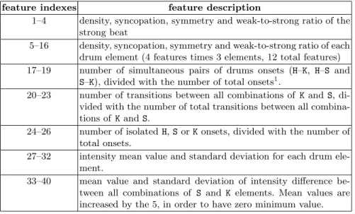
Table 1.The proposed drum features
feature indexes feature description
1–4 density, syncopation, symmetry and weak-to-strong ratio of the strong beat
5–16 density, syncopation, symmetry and weak-to-strong ratio of each drum element (4 features times 3 elements, 12 total features) 17–19 number of simultaneous pairs of drums onsets (H–K, H–S and
S–K), divided with the number of total onsets1.
20–23 number of transitions between all combinations of Kand S, di-vided with the number of total transitions between all combina-tions of KandS.
24–26 number of isolatedH,SorKonsets, divided with the number of total onsets.
27–32 intensity mean value and standard deviation for each drum ele-ment.
33–40 mean value and standard deviation of intensity difference be-tween all combinations of S and K elements. Mean values are increased by the 5, in order to have zero minimum value.
1 The total number of onsets is the number of beat subdivisions where at least
one drum element is played (in the current measure analysis, it is an integer in
2.2 Measuring Rhythm Divergence
The divergence between two rhythms is measured here by comparing the “mean relative distance” (MRD) of their feature arrays, as described in the previous paragraph. The MRD between two vectors,v1 andv2 ∈R1×k, is measured as
dMRD= 1 k k i=1 |v1(i)−v2(i)| max({v1(i),v2(i)}),
where the index i denotes the i–th element of the array. The MRD between two rhythms’ feature vectors is a real value in [0,1], with 0 meaning the same rhythm (no divergence), while higher values characterize pairs of rhythms with greater dissimilarities. It has to be noted that this divergence measure has the described functionality if all the vector elements have zero minimum value. This fact explains the addition of the constant (integer 5) to the group of features 33–40 in Table 1. The quantity of this divergence measure is not affected by each feature’s “scale” of measurement, as long as all features are between zero and an arbitrarily high value. Therefore, the MRD may be considered as a “percentage” of rhythm difference. The proposed rhythmic divergence, as has hitherto been described, disregards information about which features are actually responsible for the magnitude of the divergence. This fact allows many alternative rhythms to be considered as well fitted by the selection process, as discussed later in the analysis about fitness evaluation in Section 3.2. As a result,evoDrummer is capable of composing numerous different but equally fit rhythms, under certain user demands.
3
The Proposed GA-Based Schemes
The evolutionary strategy is a typical GA-based approach, i.e. it encompasses the standard crossover and mutation operators. However, four population ini-tialization approaches are discussed, which have different population variability potentialities. Furthermore, the chromosome representation introduces the in-corporation of intensity variations of percussive onsets, which allows the expres-sional characteristics of drum excerpts to be highlighted.
3.1 Phenotype and Genotype and Evolution of Drum Rhythms
The GA nomenclature incorporates the terms “phenotype” and “genotype” to refer to the representation of data in a given problem and the respective genetic modeling of these data. In the problem at hand, the phenotype is the represen-tation of drum rhythms, while the genotype is the represenrepresen-tation of rhythms in a form that the standard genetic operators are applicable. The phenotype is a matrix representation, called therhythm matrix, with each row corresponding to the activity of a drum element, and each column representing a certain subdivi-sion of a music measure. The number of drum elements determines the number
of rows, while the number of measure subdivisions the number of columns in the rhythm matrix. A zero matrix entry denotes that the drum in the specified row, at the beat specified by the column, remains silent (i.e. does not produce an onset). A non–zero entry denotes an onset with “intensity” defined by the magnitude of this entry. Any abstract refinement of intensities is plausible, but for the presented results we utilized 6 intensity scales, represented by integers in the set I = {1,2, . . . ,6}. Using more than 6 scales was not considered to produced a significantly richer variety in perceived intensities, as studied after careful listening by the authors. Further investigation on this subject, however, is necessary. Using these terms, a rhythm matrix can be defined as a matrix M ∈(I ∪ {0})n×m, wherenis the number of instruments, andmis the number of measure subdivisions.
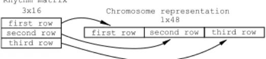
The genotype of a rhythm matrix, also referred to as chromosome represen-tation, is constructed with the serial concatenation of all its rows. The first row occupies the first part of the chromosome array and subsequent rows follow, as depicted if Fig. 1. Therefore, the chromosomeCM of a rhythm matrixMis an array with the propertyCM ∈ (I ∪ {0})1×n·m. A set of initial rhythms, which comprise the initial generation, is fed into the GA evolutionary process. New rhythms (or a new generation of rhythms) are produced, which provide better solutions to the problem at hand. Four possible population initialization schemes are discussed later. The evolution of the initial and the subsequent generations is realized through the utilization of standard genetic operators, which can be applied to a set of the aforementioned chromosome representation of rhythms, namely the following two:
1. Thecrossover operator: this operator incorporates the exchange of equally sized random parts between two chromosomes. The result is the creation of two new chromosomes, namedchildren, which encompass characteristics of both initial chromosomes, namedparents.
2. The mutation operator: mutation acts on the chromosome by assigning a random value to a random element. In the case of CM, this random value should be an integer value in{0,1, . . . ,6}.
The selection of the parent rhythms at each step of evolution is performed by a selection process that is biased towards individuals which constitute a better solution to the problem. A measurement of how good a rhythm is, in accordance to the specific problem, is realized with a fitness evaluation process which is described in the following paragraph. This work utilizes the roulette selection, according to which an individual is selected for breeding the new generation, with a probability that is proportional to its fitness.
3.2 Fitness Evaluation
A proper fitness evaluation methodology is crucial for the GA to produce effective results. The motivation of this work, as stated in Section 1, is the generation of rhythms whichdivergeby a certain amount from abase rhythm. This divergence
first row second row
third row
first row second row third row
3x16
1x48 Rhythm matrix
Chromosome representation
Fig. 1.Depiction of the rhythm matrix to chromosome transformation
is measured by the MRD, as described earlier in Section 2.2. Suppose that we have a base rhythm with afeature array denoted byrb, and a novel rhythm with afeature array denoted byrn. Suppose also that the desired divergence between the base and the novel rhythm isdd. Then, the fitness of rhythm rn according to the desired divergence is frn = |dMRD(rb, rn)−dd|, which is the distance between the desired and the observed rhythm divergence. Through evolution, the rhythms that have a fitness value closer to 0 are promoted to the next generation; thus, these rhythms have a divergence from the base rhythm which is close to the desired one. As mentioned in Section 2.2, this divergence measure does not incorporate any information about which rhythm features are responsible for its magnitude. When the user provides a base rhythm and a desired magnitude of divergence, the responses that theevoDrummer provides may encompass a large set of different rhythms. Further discussion on this issue is provided in the experimental results presented in Section 4.2.
3.3 Four Initialization Schemes
The evolutionary scheme that has hitherto been described, begins with the for-mulation of an initial generation of rhythms that breeds the next generations, creating populations of rhythms that are better fit. The paper at hand discusses four such different population initialization schemes, with different strategies on selecting a blend of random and non–random initial rhythms. Specifically, the non–random initial rhythms are copies of thebase rhythm itself. The rationale behind these schemes is to allow evolution to combine random rhythmic parts with segments of the base rhythm, creating new ones which diverge from the base rhythm by a certain amount. The random and non–random blending can be described by ablending ratio, b∈[0,1], which describes a rough percentage of random rhythms in the initial population. Therefore, if the initial population is composed of N rhythms, then the random members are [N·b], where [x] is the integer part of a real numberx.
The examined initialization schemes are the following:
1. Random: This initialization scheme is an extreme blending case whereb= 1, meaning that only random rhythms constitute the initial population. 2. Self: This initialization is the opposite of the previous case with
blend-ing ratio b = 0, where only copies of the base rhythm compose the initial population.
3. Half: The initial population comprises a fixed blend of half random rhythms and base rhythm replicates, thusb= 1/2.
4. Analog: In this initialization scheme, the blending of rhythms is proportional to the desired divergence. Specifically, the blending ratio is equal to the desired divergence measure,b=dd.
The extremeRandomandSelfinitializations are examined as test cases, in order to observe how close (or far) from the base rhythm can an initial breed of rhythms be evolved. The actual comparison that is expected to take place is presumably between theHalfandAnaloginitialization strategies.
4
Experimental Results
The experimental results aim to examine two aspects of the proposed methodol-ogy. Firstly, the efficiency of the proposed evoDrummer methodology under all the proposed initialization schemes considered, by measuring the fitness of the best individuals in several simulations. Secondly, the diversity among the best generated rhythms is analyzed, in order to measure the ability of the system to produce alternative rhythms with the desired divergence from a base rhythm. To this end, a set of six base rhythms constructed by the authors was utilized, ranging from simple to more complex rhythms. The rationale behind not us-ing random base rhythms, is the necessity to assess the system’s performance in accordance with the features produced by human–created rhythms. All the simulations described in the next paragraphs incorporated a fixed population size of 100 rhythms, a number of 100 generations, the crossover and mutation genetic operators and the roulette selection process, as described in Section 3. Furthermore, the desired divergence was considered as successfully achieved if the fitness of the best individual in a generation was below 0.0001 (error toler-ance). For each of the six base rhythms, 50 simulations were conducted in order to assess performance statistics, as well as to examine the similarity between all the generated rhythms and their characteristics. Finally, results are reported for desired divergences in the set{0 : 0.025 : 1}, which are the real numbers from 0 to 1 with an increment step of 0.025. Experimental results do not incorporate rhythm examples, since the interested reader may create as many examples as she/he wishes by using the downloadable application [4].
4.1 Adaptivity per Initialization Scheme
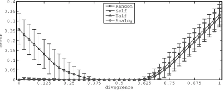
The fitness mean and standard deviations of the best fitted individuals for all desired divergences, among all 50 simulations for every rhythm are illustrated in Fig. 3. One may first notice that the fitness of the best rhythms becomes worse as the desired divergence moves from 0.625 and above for all initialization schemes. This fact highlights the lack of descriptiveness of the MRD distance, as defined in Section 2.2, when incorporating vastly different arrays. For instance, the highest value of MRD,dMRD= 1, is achieved only if one of the two measured arrays is
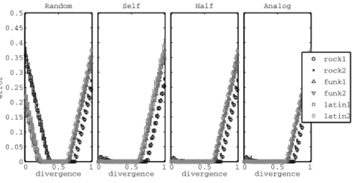
the zero array. Another notable fact is the inability of theRandominitialization process to produce rhythms which are evolved towards the base rhythm, for
all base rhythms, as depicted in Fig. 2. This fact also pinpoints that there is a vast difference between human–created rhythms and random ones, since the evolution of the latter may hardly follow the structure of the former.
0 0.5 1 0 0.05 0.1 0.15 0.2 0.25 0.3 0.35 0.4 0.45 0.5 Random divergence error 0 0.5 1 Self divergence 0 0.5 1 Half divergence 0 0.5 1 Analog divergence rock1 rock2 funk1 funk2 latin1 latin2
Fig. 2.Fitness per initialization scheme for each rhythm separately
For desired divergence with magnitude larger than 0.625, the performance of theSelf initialization scheme is the worst. This denotes that the exclusive utilization of the base rhythm itself, under several evolutionary steps (with the crossover and mutation operators as described here) is not enough to entirely alter its characteristics. This fact, along with the poor performance of the other extreme initialization methodology – the Random initialization – allows the re-jection of these two methodologies within the presented framework. Table 2 presents the mean values and standard deviations of the fitness results, catego-rized in different desired divergence groups according to the findings in Fig. 3. Therein, one may clearly observe in numeric terms the two aforementioned con-siderations about the Random and Self initializations. Additionally, it is also clear that there is a relative decrease in the low similarity divergence region (0– 0.125), compared to the middle divergence range (0.15–0.625). This may be an evidence that it is difficult to automatically devise human–like rhythms (accord-ing to the proposed features at least), even if the automatic generation process originates from the human–created rhythm itself. It also has to be noted that all the initialization techniques which used any proportion of base rhythm repli-cates, produced a perfectly fitted individual from the initial generation at the 0 divergence level, which was the base rhythm itself.
4.2 Diversity of Produced Rhythms
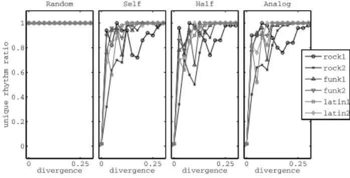
An important aspect ofevoDrummer is its ability to compose a diverse set of novel rhythms which diverge by a certain amount from the base rhythm. Two experimental measurements are utilized to evaluate this diversity, over all the desired divergences available (dd= 0 : 0.025 : 1). Firstly, the rhythm diversity is measured explicitly: for a given divergence and base rhythm, we assess a percent-age of how many unique rhythms are returned throughout the 50 simulations.
0 0.125 0.25 0.375 0.5 0.625 0.75 0.875 1 0 0.05 0.1 0.15 0.2 0.25 0.3 0.35 0.4 divegrence error Random Self Half Analog
Fig. 3.Fitness per initialization scheme for all rhythms
Table 2.Mean and standard deviation of fitnesses in several divergence regions. Best fitness in each region is demonstrated in boldface.
divergence range: 0–0.125 0.15–0.375 0.35–6.25 0.65–1.0
Random 0.1939 (0.0772) 0.0399 (0.0446) 0.0001 (0.0004) 0.1694 (0.0455)
Self 0.0022 (0.0048) 0.0003 (0.0006) 0.0006 (0.0015) 0.1844 (0.0507)
Half 0.0017(0.0027)0.0002(0.0004) 0.0001 (0.0002) 0.1705 (0.0459)
Analog 0.0021 (0.0045) 0.0002(0.0005)0.0000(0.0001)0.1690(0.0452)
This percentage is measured as theunique rhythm ratio, divided with the number of total rhythms returned by each simulation (50 in number). Therefore, the unique rhythm ratio can take a value in [50,1 1], where the extreme values denote that all rhythms are the same (value 501), or every pair of rhythms is different (value 1). Secondly, the diversity is measured through the feature difference of all the produced rhythms. The diversity of features among the 50 best rhythms returned by each simulation is measured with the mean value of the standard deviation of these features, as it is discussed more thoroughly later.
The unique rhythm ratios are illustrated in Fig. 4, for divergence values below 0.275, since above this value, almost all ratios for every base rhythm are nearly equal to 1. Additionally, the mean and standard deviation of the unique rhythm ratios for several groups of divergences are demonstrated in Table 3. These results indicate that for small desired divergences, the produced results may incorpo-rate non–unique rhythms, at some extent, except from theRandominitialization, which has the highest unique rhythm ratio value for every measured divergence. A more detailed look in Fig. 4 reveals that the simplest base rhythms consid-ered (rock1 and rock2) maintain a lower–than–unit unique rhythm ratio for divergences that approach 0.25, for all initializations exceptRandom.
The second part of the diversity analysis incorporates the assessment of the standard deviation for each feature, over all 50 simulations with a target rhythm– divergence pair. Thereafter, the standard deviation of each feature is divided with the feature’s maximum value over all 50 simulations, in order to obtain a “normalized” version of the standard deviation measurements. As a result,
0 0.25 0 0.2 0.4 0.6 0.8 1 Random divergence
unique rhythm ratio
0 0.25 Self divergence 0 0.25 Half divergence 0 0.25 Analog divergence rock1 rock2 funk1 funk2 latin1 latin2
Fig. 4.Rhythm diversity per initialization scheme. For divergence values above the depicted ones (greater than 0.275), rhythm novelty ratio is approaching 1.
Table 3.Mean unique rhythm ratios for all test rhythms in certain desired diver-gence groups. Standard deviations are demonstrated in parentheses. The initialization schemes (except random initialization) with the highest identical rhythm ratio are demonstrated in boldface typesetting.
divergence range: 0–0.125 0.15–0.275 0.3–0.425 0.45–1.0
Rand 1.0000 (0.0000) 1.0000 (0.0000) 1.0000 (0.0000) 1.0000 (0.0000)
Self 0.7161(0.3523) 0.9694 (0.0223) 1.0000(0.0000)1.0000 (0.0000)
Half 0.6811 (0.3328) 0.9717 (0.0255) 0.9994 (0.0014) 1.0000 (0.0000)
Analog 0.7033 (0.3421) 0.9733(0.0173) 0.9994 (0.0014) 1.0000 (0.0000)
the feature diversity among all simulations of a certain base rhythm–desired divergence setup, are represented by a “normalized” vector, which encompasses a description of the “relative” diversity of each feature. Consequently, the mean relative diversity, along with their standard deviation allow an overview of all the features’ diversities per desired divergence, for each base rhythm scenario. These results are depicted in Fig. 5, where the aforementioned mean value and standard deviation are demonstrated as error–bars. It has to be noted that the scale of the results (the y-axes values) does not provide any quantitative information; the informative part of this graph is the diversity changes according to divergence and base rhythm.
Feature diversity does not seem to follow any pattern with theRandom initial-ization processes. The utilinitial-ization of the rest initialinitial-ization schemes on the other hand, seems to follow a trend of increasing diversity, as divergence increases, up to one certain point. The point that the increasing trend terminates, seems to differ for different rhythm and initialization procedures. Afterwards, a descend-ing trend is observed, followed by random feature diversity fluctuations, which are compared to the ones produced by theRandominitialization scheme. Further analysis based on the findings of these graphs could reveal additional charac-teristics of the rhythms that are produced by each initialization process. This analysis can be the subject of a future work.
0 0.5 1 0 0.05 0.1 0.15 0.2 0.25 0.3 0.35 Random divergence feature diversity 0 0.5 1 Self divergence 0 0.5 1 Half divergence 0 0.5 1 Analog divergence rock1 rock2 funk1 funk2 latin1 latin2
Fig. 5.Feature diversity for different divergence values
5
Conclusions
The paper at hand introduces the methodological context that led to the con-struction ofevoDrummer, a system that utilizes interactive genetic algorithms to automatically compose novel drum rhythms. This context allows the gener-ation of novel rhythms that diverge by a certain amount from a base rhythm. According to the overall architecture employed, the user selects a base rhythm from a list of template drum rhythms and sets a desired divergence rate. There-after, the system is able to create several different novel rhythms that diverge from the base rhythm by the specified amount. To this end, the notion ofrhythm divergence is introduced, which is based on a set of drum features. The proposed features consider not only the onsets of the basic drum elements (kick, snare and hi-hat), but also their intensities which are a crucial part for the perception of drum rhythms. An evolutionary scheme based on Genetic Algorithms (GA) leads an initial population of rhythms to ones that are better fitted to the dis-cussed problem, i.e. diverge from thebase rhythm by the desired amount. Four different initialization schemes are discussed and extensive experimental results are reported, which outline the strengths and weaknesses of each methodology and the diversity of the rhythms they produce.
Future work may primarily incorporate a modification of the divergence mea-sure, the mean relative distance (MRD) of features, so that it may more ac-curately describe extremely high divergences (a problem which is discussed in Section 4.1). Afterwards, novel drum features along with an analysis on the pro-posed ones should be conducted, in order to obtain a more solid basis for rhythm similarity assessment. In parallel, the evolutionary process may be substantially assisted by the utilization of several variants of the standard crossover and mu-tation operators that were applied. Finally, a more thorough investigation on the findings of Fig. 5 should be realized, in order to examine the relations that may emerge between rhythm characteristics, as expressed by the rhythm features, and population initialization processes.
References
1. Ariza, C.: Prokaryotic groove: Rhythmic cycles as revalue encoded genetic al-gorithms. In: Proceedings of the International Computer Music Conference, San Francisco, USA, pp. 561–567 (January 2002)
2. Collins, N.M.: Towards Autonomous Agents for Live Computer Music: Realtime Machine Listening and Interactive Music Systems. Ph.D. thesis, Centre for Music and Science, Faculty of Music, University of Cambridge (2006)
3. Eigenfeldt, A.: Emergent rhythms through multi-agency in max/msp. In: Kronland-Martinet, R., Ystad, S., Jensen, K. (eds.) Computer Music Modeling and Retrieval. Sense of Sounds, pp. 368–379. Springer, Heidelberg (2008)
4. evoDrummerTestApp1 (2013),
http://cilab.math.upatras.gr/maximos/evoDrummerTestApp1.zip
5. Hoover, A.K., Rosario, M.P., Stanley, K.O.: Scaffolding for Interactively Evolving Novel Drum Tracks for Existing Songs. In: Giacobini, M., Brabazon, A., Cagnoni, S., Di Caro, G.A., Drechsler, R., Ek´art, A., Esparcia-Alc´azar, A.I., Farooq, M., Fink, A., McCormack, J., O’Neill, M., Romero, J., Rothlauf, F., Squillero, G., Uyar, A.S¸., Yang, S. (eds.) EvoWorkshops 2008. LNCS, vol. 4974, pp. 412–422. Springer, Heidelberg (2008)
6. Horowitz, D.: Generating rhythms with genetic algorithms. In: Proceedings of the Twelfth National Conference on Artificial Intelligence, AAAI 1994, vol. 2, pp. 1459–1460. American Association for Artificial Intelligence, Menlo Park (1994) 7. Kaliakatsos-Papakostas, M.A., Floros, A., Vrahatis, M.N., Kanellopoulos, N.: Ge-netic evolution of L and FL–systems for the production of rhythmic sequences. In: Proceedings of the 2nd Workshop in Evolutionary Music Held During the 21st International Conference on Genetic Algorithms and the 17th Annual Genetic Programming Conference (GP) (GECCO 2012), Philadelphia, USA, July 7-11, pp. 461–468 (2012)
8. Ravelli, E., Bello, J., Sandler, M.: Automatic rhythm modification of drum loops. IEEE Signal Processing Letters 14(4), 228–231 (2007)
9. Sioros, G., Guedes, C.: Complexity driven recombination of midi loops. In: Proceed-ings of the 12th International Society for Music Information Retrieval Conference (ISMIR), University of Miami, Miami, pp. 381–386 (October 2011)
10. Toussaint, G.T.: Generating “good” musical rhythms algorithmically. In: Proceed-ings of the 8th International Conference on Arts and Humanities, Honolulu, Hawaii, pp. 774–791 (January 2010)
11. Tutzer, F.: Drum rhythm retrieval based on rhythm and sound similarity. Master’s thesis, Departament of Information and Communication Technologies Universitat Pompeu Fabra, Barcelona (2011)
12. Yamamoto, R., Ogawa, S., Fukumoto, M.: A creation method of drum’s fill–in pattern suited to individual taste using interactive differential evolution. In: Pro-ceedings of the 2012 International Conference on Kansei Engineering and Emotion Research (May 2012)