Returns to Defaulted Corporate Bonds

(1)

Returns to Defaulted Corporate Bonds

b

H˚

akan Thorsell March 23, 2009

SSE/EFI Working Paper Series in Business Administration No. 2009:7

Stockholm School of Economics, P.O. Box 6501, SE-113 83 Stockholm, Sweden

Abstract

I test for short term excess return in a sample of 279 defaulted US corporate bonds using multiple regression analysis. There are robust excess returns after controlling for market and liquidity risk. The expected recovery rate during 2001-2006 is esti-mated to be, on average, four percentage points lower the first month after default than the present value of the recovery rate after nine months.

Key words: Bond pricing, Recovery rate JEL codes: G12, G33

b_{Financial support from the Torsten and Ragnar S¨oderberg Foundations is gratefully}

ac-knowledged. I want to thank Henrik Andersson, Magnus Dahlquist, Katerina Hellström, Tomas Hjelström, Peter Jennergren, Hanna Setterberg, Kenth Skogsvik, and Johan Söderström for helpful comments. All errors are my own.

(2)

1 Introduction

The measurement of the recovery rate helps to determine the value of bonds for going concerns. The value of a bond is the present value of the future payments, so a biased estimation of the recovery rate will bias pricing of bonds after, but also before, a default. If the recovery rate is biased, it can influence the post default returns if the bond price corrects to its intrinsic value. I study the potential bias using time series tests.

There are reasons to believe that trading is imperfect for defaulted bonds and that recovery rates might be depressed. First, some of the empirically noted results for non-defaulted bonds can survive (liquidity, default risk, and interest rate risk), or even be exacerbated by a default. Second, the market for defaulted securities can exhibit information asymmetries.

The pricing of non-defaulted corporate bonds is influenced by liquidity. Ericsson & Reneby (2003) find that bond spreads incorporate a substantial liquidity com-ponent in addition to the default risk. The less liquid a bond is in the study of Chen et al. (2005) the higher the yield spread, and De Jong & Driessen (2005) find that liquidity is a priced factor in a multi-factor model. If corporate bond prices are sensitive to liquidity before default, there is no reason to think that they are less sensitive after default. The systematic part of the default risk is priced (see Weinstein (1981), Berndt et al. (2006) or Thorsell (2008)). If the market beta is a measure of the default risk, it can be expected to increase after default. The co-variation with the market return is higher when the asset is closer to being equity. The interest rate risk is ignored here, since it is not likely a major contributor to the risk of a defaulted corporate bond.

In a default situation for a company there are new reasons for trading the securities. Some investors, such as pension funds and insurance companies, are not allowed to hold high risk assets. Other investors specialize in this type of high risk assets. This specialization could potentially create a situation of information asymmetry.1

The existence of vulture funds indicates there might be opportunities to earn good returns on distressed or defaulted assets.

Both the liquidity factor and the asymmetric information after a default event can bias the estimate of the recovery rate downwards. In general non-defaulted bonds have high probabilities of debt service and thus fairly small variations in

1 _{Financial organizations that specialize in distressed securities, such as near default or}

(3)

their expected pay-off space. The holders of defaulted corporate bonds have to find some means of knowing what their bonds are worth. A natural choice is to look at what has been recovered in earlier defaults, making the historic recovery rates the norm also for future recovery rates. The cross-sectional studies of recovery rates started with Altman & Kishore (1996). Recovery rates are now studied by the rating agencies as a matter of routine (cf. Moody’s (2007)). Altman & Kishore (1996) shows that industry and the seniority of a bond matters for the recovery rate in the cross-section. They cannot show that investment grade status, size of issue, or longevity before default has any impact on the recovery rate. The frequent studies of the cross-section can be self fulfilling, but should not influence a possible bias. That is, any pre-existing bias can be strengthened by the success of the cross-sectional studies since it is the only information available on recovery rates.

There are three common ways of defining the recovery rate of defaulted bonds in the literature:

• recovery of the face value of the bond,

• recovery of market value preceding the default, or

• an equivalent, but default-free, bond.

These three methods are all based on an instant change into a safe asset. If there are unlimited trading opportunities the three methods are equivalent. If it is not possible to immediately realize the bond, then the variation in the recovery rate of the bond is important for the economic value of a defaulted bond. The recovery rate of face value is the market price one month after default of the bond divided by the face value, and the recovery rate of market value is the market price one month after default of the bond divided by the market price one month before the default.

There are two issues that can generate bias in the recovery rate; post default risk and information asymmetry between investors. Altman & Pompeii (2003) show that the market value divided by the face value of defaulted bonds varies from 0.15 to 0.74 and differs from year to year. The bonds in their sample are the defaulted bonds that are included in the Altman-NYU Salomon Center Defaulted Bond Index. Corporate bonds typically do not have a well functioning secondary markets, so it is plausible that variation in recovery rates can have an impact on bond prices.

There are a few possible ways to figure out if there is a systematic bias in the cross-sectional default rates:

(4)

• the repayments from defaulted bonds could be summed and discounted for a net present value,

• the returns from vulture funds could be tested for excess returns, or

• the return on bonds of defaulted firms could be tested for excess returns. The repayments from defaulted firms are difficult to study since the data are typically not public and it often takes a long time until the default is resolved and/or bankruptcy is finalized. The main problem with studying vulture funds is that there is a collection of assets in the funds at any time. Some of these assets might be recently defaulted bonds, but there can be many other assets as well. The vulture fund managers may add value to the defaulted securities after default and such a study can be biased to increase the value of the assets at default. I study the return on bonds of companies that have defaulted on their securities for a limited number of months after default. There are two reasons for studying a short time period after default. First, it takes time to do value enhancing restructurings, and second, it is possible that the recovery rate is depressed by a larger than usual supply just after default.

The underlying claim that is tested in this study is straight forward;

Claim 1 The market price of a recently defaulted bond is biased

Multiple regression analysis is used to test the claim that the one month recov-ery rate estimation is biased. I calculate the cross-sectional recovrecov-ery rate (as can be compared to for instance Moody’s (2007)), and introduce time-series tests on defaulted corporate bond returns. The risk factors used to explain the excess re-turns do not in fact explain the rere-turns. This implies that there is mispricing for defaulted bond returns. Neither the common liquidity nor the Fama & French (1992) share factors have any strong bearing on the excess return after default. The estimated recovery rates ares four percent too low on average to make the excess return go away during 2001-2006.

In the next section, the model for bond values are described. In section 3 the tests and calculations that deviate from standard asset pricing tests are presented. The summary statistics of the sample and how the sample selection was done is described in section 4. The results are presented and discussed in section 5. Concluding remarks are presented in section 6.

(5)

2 Model for corporate bond value

The purpose of this section is 1) to explain how the default value of the bond relates to the before default value and 2) to describe how the bond recovery value can be compared over periods after default. The value of the bond (V) at time t

is equal to the discounted present value of the expected value of the bond value at date t+ 1.

Vt=e−rtE[Vt+1+Ct+1] (1)

For simplicity assume that the coupon is zero here (Ct+1 = 0). Defining the default

probability between t and t+ 1 as πt,t+1 and assume it is exogenous. Define the

value of the bond at timet+ 1 asVd

t+1 for the default state andVts+1in the survival

state. The value of the default state is the recovery value. The survival value of the bond is ultimately the promised payment. The states of default or survival are mutually exclusive, so equation (1) can be decomposed into:

Vt=e−rt ³ Ehπt,t+1Vtd+1 i +Eh(1−πt,t+1)Vts+1 i´ (2) The default probability of a safe bond is by definition πt,T = 0 and the safe bond

value at maturity (T) is thus equal to its face value VT = 1. The payment in

default is the object of interest, so define the payment in default function as δ :

ft+1 →Vtd+1. The set of factorsft+1 contain all information necessary to determine

the payment in default (Vd

t+1). δ can be seen as the time-varying exchange rate

between the promised payment and the payment at default, so δ(ft+1) ≤ Vts+1.

Assuming a constant probability of default (π) gives the valuation formula at time

t before default τ (t < τ): Vt=πe−rtE[δ(ft+1)] + (1−π)e−rtE h Vs t+1 i (3) and after default t > τ:

Vt=e−rtE[δ(ft+1)] (4)

Assume that creditors take over when a company defaults on its debt payments. This implies that the company is then free of all debt and there cannot be any additional defaults. Since I study only a short time after default, this should not influence the results.

(6)

face value of the bond δ(ft+1) =k1, recovery of market value δ(ft+1) = k2Vt, and

recovery in a safe bond δ(ft+1) = k3Vts+1, where k1, k2 and k3 are constants. In

the recovery of a safe bond an investor receives a fraction (k3) of a safe bond that

otherwise has the same characteristics as the defaulted bond. All three methods are point estimates. If there are risk adjusted excess returns after default it is not possible to trade the defaulted bond and get an economic value that corresponds to any of the the three methods. This transaction problem can make empirical estimates for default payments using the three methods invalid.

If liquidity is poor after default, a bond owner is exposed to the variability of the asset price and an unknown holding period. This can result in changing values of the recovery rate and a simple model of this is

δ(ft+1) =

δ(ft+q)

Q_t₊₁₊_q

i=t+1(1 +ρi)

, (5)

whereq is the number of time periods after default, andρi the discount rate. I use

the risk adjusted discount rate in a Capital Asset Pricing Model (CAPM) setting, as can bee seen in equation (8). The value of the bond at default depends on the return on the assetδ(ft+1) function and the holding period q.

3 Test method

First the recovery rates are calculated for each year for seniority and industry groups. The default time is not defined as when the bond issuer formally defaulted on the obligation, but the time when the market adapted the bond price to include the certain future default of the firm on the interest or principal.2 _{In practice this}

means that the largest negative price adjustment for each time series is defined as the default period. After default equity factors can be expected to play a larger role in explaining the expected returns and therefore market, liquidity, Small-Minus-Big (SMB) and High-Minus-Low (HML) are tested.

All returns are measured excluding the accrued interest.3 _{Only in cases where the}

2 _{The price adjustment occurs when investors realize that the company will not be able}

to service the debt. The actual default date is the date the service is due.

3 _{Even if investors’ claims on principal or interest are equivalent from an economic}

perspective, they might be treated differently in the prescription clauses of the bonds. There are instances of different prescription times for principal and interest. In addition to smaller differences in contractual treatment, Asquith et al. (1994) find that banks

(7)

bond is repaid in full does this exclusion matter. This is not common for defaulted bonds, so the impact on my results should be minimal. All tests have also been done also with returns including the accrued interest. The difference in results are minimal and if anything the inclusion of the accrued interest increases the excess return and risk adjusted discounted recovery rate.

3.1 Cross-section

The cross-sectional recovery rates are presented as averages, but calculated using OLS, since this facilitates calculating measures on variability such as the explained variation (R2_).

3.2 Time-series

To test if the market price of a defaulted bond is biased, the returns are tested for excess returns. The idea is to find out if the defaulted bonds have returns that exceed their risk compensation. A defaulted bond can be seen as something that is between debt or equity, since the true status typically is unknown at the time of default. This unknown status implies that either factors important for corporate bond pricing or equity pricing might be useful in risk adjusting the defaulted bond returns.

Factors that have been found to influence corporate bond pricing in earlier studies are tested for my sample of defaulted bonds. This means for the defaulted bonds that I test for a CAPM market risk factor and liquidity risk factors. The mar-ket risk factor can be expected to increase in significance after the default simply from the bond taking on a more equity like pay-off profile. The earlier tests are complemented with testing for liquidity risk in defaulted bonds, and construct bond liquidity factor series in Section 4.1. In addition to the test of bond factors I test factors from Fama & French (1992) which have been successful in explain-ing equity returns. Aside from the market factor, Fama and French calculates the Small-Minus-Big (SMB) and High-Minus-Low (HML) factors from a set of port-folios.

The statistical models used to test for significance of factors are standard portfolio

almost never forgive principal as part of any comprehensive debt restructuring that include subordinated public creditors.

(8)

tests, with portfolio formation dependent on industry and seniority. The estimation equation can be seen in equation (6),

Rt−Rft =α+βFt+²t, (6)

here Rt is the simple return on a bond at time t, Rf is the risk free return, Ft is

a vector of factors, and ²t is the error term. All tested factors are not zero cost

portfolios. This implies that for the non zero cost portfolios the average value of the factors can influence the estimated intercept, and hence the estimated excess return. As it turns out, this is not a problem.

The portfolios are equally weighted, since the market capitalization cannot be determined from my data set. Studies on equity portfolios use typically use value-weighted portfolios. The choice of equally value-weighted portfolios can give smaller issue bonds a relative large impact on the results.

3.3 Present value of recovery rates

To estimate the economic significance of the post default variations in the recovery rate, the present value of the recovery rate of face value (market price of the bonds divided by their face value) after default is calculated. The interest rate for market risk is adjusted to see if the estimate forδτ+nover time differs from the “at default”

recovery rates for both book and market values. The discounting is presented below in equation (8).

Defaulted bonds are assets which need to generate risk adjusted returns for in-vestors to hold them. There should be an insignificant excess return (alpha) and insignificant betas if the use of a risk free asset as a proxy for the recovery value is a good assessment. The variability in price of the safe asset is by nature small, and the default probability is also small (empirically fractions of percent per month). If the value in default is too depressed, then there should be excess returns in the months following the default. These excess returns are the fingerprints of the too low recovery rate. The sample is randomly divided into two groups to avoid discounting with in-sample betas. The first group is used to calculate betas for industry and seniority,

Rtj−Rtf =αj+βjFt+²t, (7)

whereRj_t is the return on bondj at timet,Rf_t is the risk free return,Ft is a vector

of factors, and ²t is the error term. Time (t) runs from the time of default (τ) for

(9)

the next equation.

The second group is used to calculate the out-of-sample present value of the equiv-alent recovery rate of face value (RR= CleanP rice

F aceV alue). This operation is done to make

the recovery rates comparable over time. Note that the excess return test is suf-ficient to answer the question of bias in the recovery rate at default. The present value of the recovery rates is calculated as,

P V(RRτ+n) =

RRτ+n

Q_τ₊_n

i=τ(1 +Rfi + ˆβFi)

, (8)

where alpha is assumed to be zero and beta ( ˆβ) is the mean estimated parameter from the first group4 _{estimated in accordance with equation (7). Equation (8) is}

used to calculate the present value up to nine months after default (n). The reason for this relatively short period is that the tests are if the recovery rate might be depressed at the time of default, not if there is a drift in the asset value.

4 Data

The sample consists of 134 companies with 279 defaulted bond price series. No company has issued more than 4 percent of the bonds in the sample. The sample is collected from the Thomson/Datastream database. All bonds in the sample have fixed coupons. The sample period covers six years from 2001 to the end of 2006. A problem with corporate bond data is typically thin trading. For the average bond in the Datastream sample, trade volume is registered in the ISMA TRAX system5 _{in 14 percent of all months. The average traded volume (nominal) for a}

traded bond is 7.8 MUSD per month. The traded volume is on average about 264 MSUD per month in the sample. The median bond issue has an amount issued of 200 MUSD.

Datastream does not only rely on the TRAX system for price information, but mainly source their corporate bond data from FT Interactive Data (FTID). FTID

4 _{Each bond is assigned a post-default beta in accordance with what grouping it belongs}

to.

5 _{ISMA (the International Securities Market Association) is the self-regulatory}

organi-zation and trade association for the international securities market (including the Eu-robond market). ISMA TRAX is the ISMA trade matching and regulatory reporting system for the OTC markets.

(10)

uses market transactions and calculates prices using, amongst other things, bid information from their fund clients. According to FTID; prices are calculated to reflect verifiable information to the extent that it is formative for the good faith opinion of FTID as to what a buyer would pay for the bond in a current sale. The price information has a tendency to go stale after the default, i.e. the same price is repeated during several time periods in the data set. If there is a problem with stale prices, the intercepts in the CAPM tests are negative since there is a financing cost (Rf_{), but no income from the bond. The default event seems to}

create volume. The average turn-over five months after default is 24 percent higher than the average turnover five months before default, measured in terms of face value. Using the, potentially, stale clean prices favors finding no positive excess return, or lower discounted recovery rates since coupons are excluded.

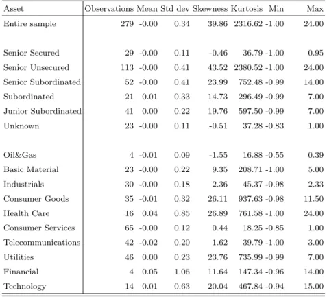
Summary statistics for the sample of defaulted bond are presented in Table 1.

Table 1. Monthly sample returns during ten month before default and ten months after default.

Asset Observations Mean Std dev Skewness Kurtosis Min Max Entire sample 279 -0.00 0.34 39.86 2316.62 -1.00 24.00 Senior Secured 29 -0.00 0.11 -0.46 36.79 -1.00 0.95 Senior Unsecured 113 -0.00 0.41 43.52 2380.52 -1.00 24.00 Senior Subordinated 52 -0.00 0.41 23.99 752.48 -0.99 14.00 Subordinated 21 0.01 0.33 14.73 296.49 -0.99 7.00 Junior Subordinated 41 0.00 0.22 19.76 597.50 -0.99 7.00 Unknown 23 -0.00 0.11 -0.51 37.28 -0.83 1.00 Oil&Gas 4 -0.01 0.09 -1.55 16.88 -0.55 0.39 Basic Material 23 -0.00 0.22 9.35 208.71 -1.00 5.00 Industrials 30 -0.00 0.18 2.36 45.37 -0.98 2.33 Consumer Goods 35 -0.01 0.32 26.11 937.63 -0.98 11.50 Health Care 16 0.04 0.85 26.89 761.58 -1.00 24.00 Consumer Services 65 -0.00 0.12 0.44 18.25 -0.85 1.00 Telecommunications 42 -0.02 0.20 1.62 39.79 -1.00 3.00 Utilities 46 0.00 0.23 23.76 735.99 -0.99 7.00 Financial 4 0.05 1.06 11.64 147.34 -0.96 14.00 Technology 14 0.01 0.63 20.04 467.84 -0.94 15.00

This table presents returns from a sample of 279 defaulted corporate bonds. The bonds are collected from Thomson/Datastream. The return for each bond-month is the clean price return (Pt−Pt−1

Pt−1 ). The seniority of the bonds have been identified

from the EDGAR database. Bonds where the seniority has been unclear are classified as Unknown. The classification into industries follow the ICB standard.

(11)

There is a large negative return in each bond return series (the default) and this influences all moments of the return series. The mean return for the entire sample is negative, but some groups have positive mean returns. The standard deviations are high compared to the mean returns, the skewness is positive and the kurtosis is high.

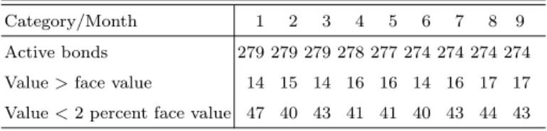
The sample characteristics for the defaulted bonds can be expected to be different from a random sample of corporate bonds. The reason is that a random sample contains few defaults compared to this sample. Nine months after default six per-cent of the defaulted bonds have a clean price higher than their face value. Sixteen percent have a clean price lower than two percent of their face value.

Table 2. Bounce back and drop dead bonds after default.

Category/Month 1 2 3 4 5 6 7 8 9

Active bonds 279 279 279 278 277 274 274 274 274 Value>face value 14 15 14 16 16 14 16 17 17 Value<2 percent face value 47 40 43 41 41 40 43 44 43 This table presents the number of bonds that recover after default and the number of bonds that are valued at less than 2 percent of face value up to nine months after the default event.

4.1 Liquidity measures

The liquidity risk has been shown to be important for the pricing of corporate bonds. There are many ways to operationalize the liquidity measure; three ways are measures of traded volume, market impact of a large transaction, and the size of the difference between the bid and ask spreads. The available data has low frequency (monthly) and contains only prices and traded volumes, so the return and volume based liquidity measures are used. Two share price based factors are tested. The idea with the share price based factors is that they capture general sensitivity of asset prices against systematic liquidity risk. Finally two measures are calculated from a sample of 3,774 U.S. corporate bond price series.

The two share based series are calculated according to Sadka (2006) and P´astor & Stambaugh (2003). Both these series are available from 2001 through 2005. The P´astor and Stambaugh series are based on a volume reversal coefficient. They find that their market wide liquidity factor is priced. To complement the share price based liquidity measures, measures for liquidity risk are calculated from the sample of corporate bond returns.

(12)

From the sample of corporate bond price series innovations are calculated in line with what P´astor & Stambaugh (2003) does for the stock market. Monthly data give a limited number of data points. The idea is to calculate the return response to trading volume. The response coefficient for each bond (i) is calculated using the OLS regression,

r_i,te ₊₁ =θi+φiri,t+γisign

³

re_i,t´·vi,t +²i,t, (9)

wheresign(·) is a function that takes on -1 or 1 depending on the sign of the input, and the variables are defined as in P´astor & Stambaugh (2003):

ri,t: the clean price return on bond i in montht

re

i,t: ri,t−rm,t, where rm,t is the average clean price return on all the

bonds in the sample during month t,

vi,t: the nominal traded volume reported in the TRAX system for bond

i in month t, and

²i,t: the residual

The gamma (γ) coefficient is the excess return response to trading volume. The

sign(·) function eliminates the difference between positive and negative excess re-turns, making the coefficient linear in absolute volume. The underlying economic idea is that an increase in trading volume inflates the return in the first time pe-riod and when the trading volume decreases in the next time pepe-riod the returns decrease, i.e. a return reversal. If this idea is correct the gamma can be expected to be negative on average. High trading volumes should be associated with negative excess returns in the next time period.6 _{Only bond month observations where}

there is trade volume reported in TRAX are included in the regression. Monthly return observations with abnormally high (+10%) and low (-10%) returns are ex-cluded. This gives 1,745 coefficient estimates for the entire period. For each time period the average gamma estimate is calculated,

ˆ γt = 1 N N X i=1 ˆ γi,t. (10)

The average return response coefficient is a measure of how large the average return

6 _{This is true, the mean} _γ _{for all bonds in the sample is negative -2.0e-009 with a}

(13)

reversal is in the next time period. P´astor & Stambaugh (2003) have a problem with an upwards trend in their sample of NYSE and AMEX bonds. My shorter sample period does not exhibit this problem, and it does not have significant serial correlation7_{, so the innovation is calculated in a similar manner, but exclude the}

dollar value scaling quota,

∆ˆγt=a+b∆ˆγt−1+cγˆt−1+ut (11)

The regression in equation (11) produces serially uncorrelated residuals. The resid-uals are the part of the changes in return response coefficients that does not depend on earlier changes or levels of return response coefficients. The idea is to clean the return response innovations from time series dependencies.

I calculate the innovation (Lt) in liquidity from the residuals (ut),

Lt=

1

100uˆt (12)

The re-scaling by 100 is done to follow P´astor & Stambaugh (2003), but is not necessary for the bond series, since the traded volumes typically are large in com-parison to the returns. The effect of not re-scaling means that the factor values are very small and that there will be some very large liquidity beta estimates. In addition to the share based series and the above bond liquidity measure, a second bond liquidity measure, AILLIQ, is calculated in line with Amihud (2002).8 _More

precisely, the AILLIQ measure is defined here as

AILLIQt = 1/Nj N j X k=1 |rk,t| vk,t , (13)

whereNj is the number of bond observations in month t,rk,t is the clean price net

return for bond k during period t, and vk,y is the reported daily average nominal

volume in the TRAX system.AILLIQtis thus the average quota between absolute

7 _{The first order serial correlation is 0.20, slightly below P´astor and Stambaugh’s 0.22,}

but not significant.

8 _{Both bond series are calculated from February 2001 through 2006. Amihud sums}

over days when there has been trading, while here only the months when the TRAX system has reported trading volume is used in the cross-sectional calculations. Amihud calculates the absolute mean average daily return and here the absolute monthly return is calculated from clean prices, ignoring the possible effect of the accrued coupon.

(14)

clean price return and reported transaction volume. In the first month included (February 2001) there are 72 quotes. This is the smallest number of quotes in the sample and the maximum is 1,011.

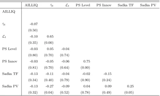
The measures for liquidity risk are all based on changes in return in relation to trading volumes. The pair wise correlation between the series is calculated, to see if there are similarities between the different liquidity series.

Table 3. Pairwise correlation between liquidity measures.

AILLIQ γˆt Lt PS Level PS Innov Sadka TF Sadka PV

AILLIQ ˆ γt -0.07 (0.50) Lt -0.10 0.65 (0.35) (0.00) PS Level -0.03 0.05 -0.04 (0.80) (0.70) (0.74) PS Innov -0.03 -0.05 -0.06 0.75 (0.81) (0.70) (0.64) (0.00) Sadka TF -0.13 -0.11 -0.04 -0.02 -0.15 (0.34) (0.40) (0.79) (0.90) (0.24) Sadka PV -0.13 -0.27 -0.09 0.04 0.09 0.25 (0.32) (0.04) (0.52) (0.78) (0.49) (0.05)

This table presents the pairwise correlations between the different measures of liquidity. The measures are the AILLIQ measure, as calculated in equation (13), the ˆγt, as calculated in

equation (10). The Lt is the innovations in liquidity in the bond market, as calculated in

equation (12). The two PS series (Level and Innov) are the level and innovations for the stock market in accordance with P´astor & Stambaugh (2003). The two Sadka series are fixed (TF) and variable (PV) price effects, calculated according to Sadka (2006). In parenthesis below each pairwise correlation is the significance level.

The bond based series (AILLIQ, ˆγt, andLt) have insignificant and mostly negative

correlations with the share based series. Only a few of the correlations are signifi-cantly different from zero. The liquidity series seems to measure different aspects of liquidity since they are different from each other. The implication is that all liquidity measures needs to be used in the later tests.

4.2 Institutional setting

(15)

• the company fails to pay interest on the due date,

• the company fail to pay the principal on the due date,

• the company breaches any other covenants or warranties connected to the secu-rities and the failure continues, or

• the company declares itself in bankruptcy, insolvency or reorganization.

Investors can purchase corporate bonds at issue or in the secondary market. On the secondary market corporate bonds are either traded over-the-counter or through an exchange. Only some of the corporate bonds that are traded through an exchange are formally listed. More than 60 percent of the bonds in the sample are quoted and traded at the New York Stock Exchange (NYSE). Most of the bonds in the sample (at least 233 out of 279) have equities listed on one of the U.S. exchanges. The companies that have listed equity are required to follow standard disclosure and reporting regulations. There is no listing agreement for a debt issuer on NYSE, but the regulations for listed companies state that the issuer must release all relevant information immediately upon determining that the interest or principal will not be paid in full.

Firms in financial distress have a number of options for how to avoid bankruptcy. The two main options are to do an informal restructuring with the creditors or to file for bankruptcy protection under Chapter 11 of the U.S. bankruptcy code. Asquith et al. (1994) finds that only 42 of their 102 financially distressed firms file for bankruptcy. The firms try to avoid going into Chapter 11 since the process is costly. The way firms handle their distress situation is important for the value of the defaulted bonds.

5 Results

5.1 Cross-section

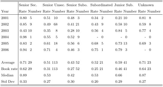
The cross-sectional recovery rates are in line with the data of other studies, for instance by Altman & Kishore (1996) or the yearly Moody’s report. Moody’s has a larger sample since they include bonds from several countries. The figures here include only US corporate bonds, so the parameters differ somewhat from Moody’s. In Table 4 through 6 the recovery rate based on market value grouped by seniority and industry is calculated.

(16)

Table 4. Average market value recovery rate on defaulted corporate bonds per year by seniority.

Senior Sec. Senior Unsec. Senior Subo. Subordinated Junior Sub. Unknown Year Rate Number Rate Number Rate Number Rate Number Rate Number Rate Number

2001 0.80 5 0.51 10 0.48 3 0.34 2 0.21 10 0.81 8 2002 0.85 9 0.49 68 0.41 21 0.43 9 0.58 10 0.59 8 2003 0.43 10 0.35 8 0.28 10 0.56 4 0.84 5 0.77 4 2004 0.98 1 0.55 5 0.52 9 - 0 - 0 - 0 2005 0.83 2 0.61 18 0.56 6 0.68 5 0.73 13 0.69 3 2006 0.94 2 0.71 4 0.46 3 0.75 1 0.79 3 - 0 Average 0.71 29 0.51 113 0.43 52 0.52 21 0.59 41 0.71 23 Book rate 0.62 29 0.31 113 0.27 52 0.25 21 0.46 41 0.64 23 Median 0.89 0.53 0.42 0.53 0.66 0.87 Std Dev 0.33 0.27 0.30 0.20 0.29 0.27

This table presents the average recovery rate for defaulted bonds. The recovery rate is cal-culated from clean prices as 1 +Pt−Pt−1

Pt−1 . TheR

2_{and ¯}_R2_{for the entire sample are 9.7 and}

8.1 per cent respectively. The book rate is the average clean price on the month after default divided by the par value. Each estimate is followed by the number of observations used to calculate it.

The seniority of a corporate bond is an indicator for the level of the recovery rate. There is a pattern where both the average market and the book recovery rate are higher for the senior bonds and the junior subordinated bonds. There is a smile pattern in the average recovery rate. The explained variation (R2_{) is 9.7 percent}

for the entire sample, indicating a considerable variation around the means. If regressions are run for each individual year, the R2 _{is about 80-90 percent. This}

difference in explained variation indicates that the time variation in recovery rates is high.

The recovery rates of face value are lower than the recovery rates of market value. There are two reasons for this. First, the recovery rate of face value incorporates all price adjustments before the default and the recovery rate of market value only what is lost during the month of default. Second, the recovery rate of market value is calculated with a smaller denominator, due to the partial adjustment in price. The lower recovery rate of face value indicates that the market has anticipated the defaults to some extent.

I divide the sample into the ten ICB sector code industries and present the average recovery rate of market value in Table 5.

(17)

Table 5. Average market value recovery rate on defaulted corporate bonds per year by industry.

Oil&Gas Basic Indust. Consumer Health Consumer Telecom Utilities Financial Tech. Material Goods care services

Year Rate Nr Rate Nr Rate Nr Rate Nr Rate Nr Rate Nr Rate Nr Rate Nr Rate Nr Rate Nr 2001 - 0 0.41 4 0.65 3 0.20 2 - 0 0.78 8 0.37 4 0.48 15 0.78 1 0.17 1 2002 - 0 0.51 4 0.50 16 0.63 6 0.55 9 0.60 24 0.38 36 0.64 20 0.19 3 0.48 7 2003 0.68 2 0.48 12 0.24 5 0.41 4 0.29 3 0.69 12 0.05 2 - 0 - 0 0.20 1 2004 0.87 2 0.28 2 0.47 2 0.45 5 0.04 1 0.98 2 - 0 0.98 1 - 0 - 0 2005 - 0 0.80 1 0.82 2 0.58 10 0.88 3 0.68 18 - 0 0.72 9 - 0 0.34 4 2006 - 0 - 0 0.61 2 0.64 8 - 0 0.93 1 - 0 0.95 1 - 0 0.95 1 Average 0.77 4 0.47 23 0.50 30 0.54 35 0.53 16 0.68 65 0.36 42 0.62 46 0.34 4 0.43 14 Median 0.83 0.55 0.59 0.62 0.56 0.66 0.28 0.74 0.27 0.39 Std Dev 0.23 0.28 0.32 0.32 0.29 0.21 0.24 0.31 0.32 0.30

This table presents the average recovery rate for defaulted corporate bonds. The recovery rate is calculated from clean prices as 1 + Pt−Pt−1

Pt−1 . TheR

2 _{and ¯}_R2 _{for the entire sample are 14.6}

and 11.7 per cent respectively. Each estimate is followed by the number of observations used to calculate it.

The results from the industry based sample are similar to the results from the seniority sample, with low panel R2 _{and high yearly} _R2_{. Each year in general}

has only a few data points, so it is not possible to draw any conclusions on the distribution or time variation from this grouping.

Firms in different industries typically have different compositions of assets. The recovery rates grouped by seniority and industry are presented in Table 6.

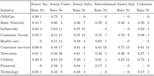
Table 6. Average market recovery rate on defaulted corporate bonds by seniority and industry.

Senior Sec. Senior Unsec. Senior Subo. Subordinated Junior Sub. Unknown Industry Rate Nr Rate Nr Rate Nr Rate Nr Rate Nr Rate Nr

Oil&Gas 0.90 1 0.73 3 - 0 - 0 - 0 - 0 Basic Material 0.41 7 0.60 3 0.46 7 0.59 2 0.48 2 0.39 2 Industrials 0.63 3 0.64 11 0.37 15 - 0 - 0 0.62 1 Consumer Goods 0.49 1 0.51 11 0.37 13 0.75 1 0.79 8 0.98 1 Health care - 0 0.51 11 0.58 4 0.65 1 - 0 - 0 Consumer services 0.69 6 0.58 17 0.61 6 0.61 10 0.75 13 0.81 13 Telecomm. 0.91 1 0.34 28 0.81 1 0.42 5 0.30 6 0.27 1 Utilities 0.92 9 0.61 19 0.29 1 0.01 1 0.43 12 0.74 4 Financial - 0 0.58 2 0.04 1 0.17 1 - 0 - 0 Technology 0.95 1 0.42 8 0.38 4 - 0 - 0 0.17 1

This table presents the average recovery rate for defaulted bonds. The recovery rate is calculated from clean prices as 1 +Pt−Pt−1

Pt−1 . TheR

(18)

TheR2 _{is naturally high since there are many explanatory variables to data points.}

When this is adjusted for in the ¯R2_{the explanatory value drop considerably. There}

are even fewer data points per grouping.

The cross-sectional recovery rates are in line with earlier results. There is some time variation, as can be seen in Table 4. A different type of time variation is the theme of the next section, the after default time variation.

5.2 Time-series

Time-series of defaulted bond returns are problematic, since they contain both stale prices and ’dead cat bounces’.9 _{Stale prices will in this setup give zero}

re-turns on the bond and make it harder to find excess rere-turns. In later periods when the potentially stale price adjusts, it is easier to find excess returns. Cross-sectional smoothing should alleviate this problem. For a schematic overview of what hap-pened to the mean returns of defaulted corporate bonds I include Figure 1. The mean excess return in Figure 1 is calculated asRτ = _N1

P

i=1...N(Rτ,i−Rfτ)), where

N is the number of bonds, τ is the time period, Rτ,i return on bond i, and Rfτ

the risk free rate. The cumulative mean excess return is the cumulative sum of the presented mean excess returns.

−10 −5 0 5 10 −0.5 −0.4 −0.3 −0.2 −0.1 0 0.1 0.2

Mean excess return.

Excess monthly return

Event time (months)

−10 −5 0 5 10 −0.6 −0.5 −0.4 −0.3 −0.2 −0.1 0 0.1

Cumulative mean excess return.

Cumulative excess monthly return

Event time (months)

Fig. 1. Mean excess return on defaulted corporate bonds 2001-2006.

The mean excess return from corporate bonds is negative before the default occurs, implying that investors adjust their pricing before the default. This adjustment can

9 _{A dead cat bounce is when a moderate rise in the price of a stock follows a spectacular}

(19)

also have happened for many bonds not entering into the default state, so it does not necessarily carry any information. More interesting is that, as can be seen in Figure 1, the mean excess return is consistently positive after the default. The fairly sharp rise in returns in the months after the default implies that there might be an overshooting effect, at least for the mean excess return.

The positive mean excess return after default raises the question of what bonds perform well after the default. Is it the same bonds that consistently do well in a turnaround situation? To answer this question I rank the sample into deciles depending on their return one month after the default.

Table 7. Average excess return in decile portfolios after default.

Portfolio/Month 1 2 3 4 5 6 7 8 9 10 Mean ρ Portfolio 1 -0.38 0.94 0.07 -0.24 0.11 -0.14 0.16 -0.01 0.05 0.16 0.07 -0.39 Portfolio 2 -0.15 0.02 0.06 0.18 0.09 -0.02 0.02 0.02 0.07 0.09 0.04 0.20 Portfolio 3 -0.07 -0.04 0.01 0.10 0.02 0.04 0.04 0.09 0.01 0.02 0.02 0.28 Portfolio 4 -0.02 0.01 0.05 0.06 0.06 0.04 -0.01 0.03 0.03 0.00 0.02 0.33 Portfolio 5 -0.00 0.03 0.52 0.06 0.06 0.01 0.02 -0.01 0.57 0.03 0.13 -0.27 Portfolio 6 -0.00 -0.05 -0.02 -0.05 0.00 0.00 0.42 0.00 -0.02 0.01 0.03 -0.03 Portfolio 7 0.02 0.02 0.00 -0.00 -0.02 0.05 0.02 0.00 0.01 0.02 0.01 -0.15 Portfolio 8 0.06 -0.02 0.02 0.01 -0.00 0.04 0.02 -0.01 0.02 0.04 0.02 -0.36 Portfolio 9 0.18 -0.04 0.04 0.02 -0.01 0.10 0.02 0.06 0.06 0.02 0.05 -0.43 Portfolio 10 1.15 0.01 -0.01 0.00 0.01 0.00 0.05 0.07 0.01 0.02 0.13 -0.02 Mean 0.08 0.09 0.07 0.01 0.03 0.01 0.08 0.02 0.08 0.04 0.05 -0.04 This table presents the average clean price excess return for decile portfolios ranked on log excess return the month after default. The average log excess return for each decile portfolio is presented for ten months following the default.ρis the first order autocorrelation coefficient for the mean excess returns in each portfolio.

From the mean excess returns per portfolio in Table 7 it is not evident that some bonds will recover more than others, or that there is any pattern from the return ranking. Longer ranking periods have been tested, but the results are similar with no clear pattern in the cross section. The median variability for the portfolio returns is 0.04, with three outliers (Portfolios 1, 5, and 6). The potential turn around in excess returns after default is present in all ten portfolios. The strong excess return could be explained by risk. The correlations are fairly large, but not significant.

5.2.1 Risk explanations

Two risks for corporate bonds can be expected to survive a default; the market and the liquidity risks. The market risk could even be expected to increase since

(20)

the bond after default has a pay-off profile more resembling a share. Predicting how the liquidity risk should change is not as clear cut. The increase in volume after default decreases the risk associated with selling the bonds, but trading on asymmetric information could increase the risk.

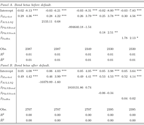
The initial test on the entire sample of defaulted corporate bonds is presented in Table 8 below. I test for excess returns before and after the default event. All the liquidity factors calculated in section 4.1 are used, but only four of them are presented in Table 8. The excluded ones are not significant and the intercept and market beta are no different than the ones presented in Table 8. The risk factors of Fama & French (1992) are also used as additional controls, and reported in Table A.1 in Appendix A. The results are similar to the ones in Table 8, where the SMB and HML coefficients are significant before default but only HML after. The intercept and market beta are only marginally different when the SMB and HML factors are included.

(21)

Table 8. Return beta representation for the one-factor model and the liquidity factor. Panel A. Bond betas before default.

Intercept -0.02 -8.13 *** -0.03 -6.21 *** -0.03 -8.31 *** -0.02 -8.00 *** -0.03 -7.83 *** βM arket 0.29 4.36 *** 0.28 4.22 *** 0.26 3.79 *** 0.25 3.78 *** 0.30 4.56 *** βAILLIQ 2133.11 0.68 βP&SBond -894640.18 -1.54 βP&SStock 0.18 2.51 ** βSadka 1.78 2.13 * Obs. 2387 2387 2349 2330 2330 R2 _0.01 _0.01 _0.01 _0.01 _0.01 ¯ R2 _0.01 _0.01 _0.01 _0.01 _0.01

Panel B. Bond betas after default.

Intercept 0.05 4.08 *** 0.06 4.03 *** 0.05 4.05 *** 0.05 3.98 *** 0.05 3.64 *** βM arket 0.49 4.42 *** 0.46 3.99 *** 0.49 4.41 *** 0.53 4.53 *** 0.52 4.14 *** βAILLIQ -10379.89 -1.60 βP&SBond 1810131.86 0.74 βP&SStock -0.06 -0.34 βSadka 0.04 0.02 Obs. 2707 2707 2707 2395 2395 R2 _0.00 _0.00 _0.00 _0.00 _0.00 ¯ R2 _0.00 _0.00 _0.00 _0.00 _0.00 Re₌_α₊_βF₊_ε

In this table the one-factor model, and two-factor liquidity models, are tested on a sample of defaulted bonds, measured in default time. Panel A consists of the estimated coefficients before the default event and Panel B consists of the estimated coefficients after the default. The data is pooled for ten months before default (Panel A) and ten months after default (Panel B). The market beta (βM arket) uses the

market factor of Fama & French (1992). The liquidity measures are based on Amihud (2002), P´astor & Stambaugh (2003) and Sadka (2006). The specifications of the liquidity measures are described in Section 2.4.1, equations (12) and (13). The t-statistics are calculated using robust standard errors. ***, **, and * denotes significance on the 1, 2.5, and 5 percent level.

Two of the liquidity risk factors are significant before the default event. None of the liquidity factors are significant after default. Either the measures of liquidity risk do not influence pricing for bond in default, or the measures are inadequate for capturing the liquidity risk. The AILLIQ and P&S Bond betas are very large, as anticipated.10 _{However, they do not seem to influence the size of the intercept}

much and are insignificant, so the potential problem with bias in the intercept is most likely minor.

The intercept in Panel A is negative, indicating that bonds have poor returns before

(22)

a possible default. The estimated betas are high for corporate bonds (0.25-0.30) compared to betas for going concerns estimated by Weinstein (1981) (mean betas against stock market 0.03-0.21 during 1964-1972) or Thorsell (2008) (0.06 during 2001-2005). Now, these bonds are part of a choice based sample, and do default but this pattern could be present in other bonds as well, so it is not a certain indicator of imminent default. The risk measures in the test do not do a good job at capturing the variability, as measured by the R2 _{(1 percent). The intercepts}

and the market betas are all significantly different from zero, but the liquidity coefficients are not. The low significance of the liquidity coefficients is puzzling, considering that trading volumes tends to increase both before and after default, and that liquidity risk is a common explanation for corporate bond returns. The liquidity factors have only slightly higher significance if the market beta is left out of the regressions. Hence it is not the market beta that crowds out the liquidity factors.

After the default event, in Panel B, the sample can be considered to be a ran-dom selection of defaulted bonds. The intercepts turn positive (0.05-0.06) and are significant. Considering that the intercepts are the average monthly unexplained excess return, they are very high. The median unexplained excess return is about 1.6 percent per month. This difference between mean and median indicates that the distribution is non-normal. The robust standard errors of White (1980) are used to decrease the problem of non-normality. The market beta increases to 0.46-0.53, as could be expected from the bond becoming more equity-like. The variance in the clean price returns increases from a mean of 0.03 before default to a mean of 0.43 after default, more than ten fold. As could be expected from the significant intercept and insignificant parameter estimates the R2 _{is zero.}

The weak performance of the tested risk factors and the large positive intercept from Table 8 indicates that a portfolio of defaulted bonds acquired at default generates excess returns. The spread of returns in Table 7 is fairly even, and it looks like most defaulted bonds have an expected positive return. The tentative conclusion is that the average bond is underpriced in the default month, and that at least the risks I have tested are not the reason for this under pricing.

Market risk, but not liquidity risk, seems to be important for the pricing of de-faulted bonds. The large variation in post default returns and earlier cross-sectional results on industries and seniority give cause to investigate if the risk profile differs in these dimensions.

(23)

5.2.2 Seniority

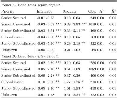
The priority in bankruptcy determines how much of a bonds value is recovered in bankruptcy. The different priority bonds typically get paid in different fractions, see Table 4. The standard deviation also differs between the different priorities. It could thus be expected that both the intercept and the market beta varies depending on priority ranking. The data on the priority ranked portfolios is presented below in Table 9.

Table 9. Return beta representation for seniority ranked portfolios. Panel A. Bond betas before default.

Priority Intercept βM arket Obs. R2 R¯2

Senior Secured -0.01 -0.73 0.10 0.63 249 0.00 0.00 Senior Unsecured -0.03 -6.07 *** 0.38 3.93 *** 1019 0.01 0.01 Senior Subordinated -0.03 -3.71 *** 0.33 2.14 ** 469 0.01 0.01 Subordinated -0.04 -2.60 *** 0.19 0.65 163 0.00 0.00 Junior Subordinated -0.03 -5.36 *** 0.28 2.18 ** 322 0.01 0.01 Unknown 0.00 0.09 0.21 1.02 165 0.01 0.00

Senior Secured 0.02 2.39 *** 0.10 0.65 286 0.00 0.00 Senior Unsecured 0.05 2.10 ** 0.51 1.09 1083 0.00 0.00 Senior Subordinated 0.09 2.28 ** -0.37 -0.39 496 0.00 0.00 Subordinated 0.10 2.20 ** 1.77 1.76 * 210 0.01 0.01 Junior Subordinated 0.05 2.10 ** 1.01 1.93 * 410 0.01 0.01 Unknown 0.01 1.58 0.41 2.24 ** 222 0.02 0.02 Re₌_α₊_βF₊_ε

In this table the one-factor model is tested on a sample of defaulted bonds, measured in default time. Panel A consists of the estimated co-efficients before the default event and Panel B consists of the estimated coefficients after the default. The data is pooled for ten months before default (Panel A) and ten months after default (Panel B). The market beta (βM arket) uses the market factor of Fama & French (1992). The

t-statistics are calculated using robust standard errors. ***, **, and * denotes significance on the 1, 2.5, and 5 percent level.

The tests for the priority ranked sample in Table 9 have similar results as the entire sample in Table 8. The exception is that the market beta only is significant for a few of the priority groups before default. The intercept seems to increase with lower priority, indicating that the more insecure bonds are more mispriced at default. The explained variation (R2 _{and ¯}_R2_{) is still low, indicating that the risk,}

as measured by the tested factors, has little to do with the returns post default. I have tested the Fama & French (1992) factors and they are not significant after default, confirming the general results in Table 8.

(24)

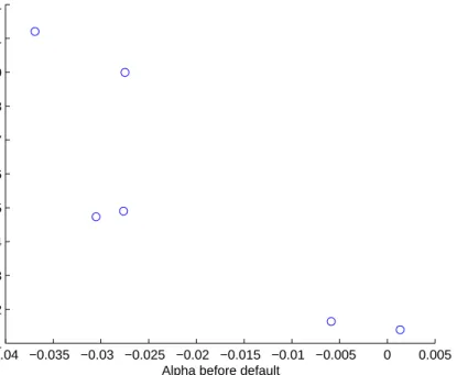
The intercepts for the seniority groups are negatively correlated before and after default. This is shown for the seniority grouped sample in Figure 2 below. The

−0.04 −0.035 −0.03 −0.025 −0.02 −0.015 −0.01 −0.005 0 0.005 0.01 0.02 0.03 0.04 0.05 0.06 0.07 0.08 0.09 0.1 0.11 Seniority groups.

Alpha after default

Alpha before default

Fig. 2. Intercepts before and after default for seniority grouped sample.

negative correlation before and after default is valid for the entire sample, and to a lesser degree for the industry and return ranked groups. The individual bond be-fore default alphas regressed on corresponding after default alphas give a negative coefficient of -0.6. The alphas after default are on average positive, so either the negative correlation is a sign of an over-shooting effect (mispricing) or there are unknown risks that are not controlled for. To the extent that the risks in Table 8 and Table A.1 are controlled for the intercept is still significant and positive. If the explanation is mispricing, then the size of the over-shooting is different for different seniorities. The senior subordinated bonds has a low after default alpha, and less certain categories have larger after default alphas. An economic interpre-tation of this correlation is that junior bonds are hurt more than senior bonds by the uncertain prospects before default. After default the junior bonds benefit more from resolution of uncertainty.

5.2.3 Industry

The sample is divided into industry portfolios and test for market risk in Table 10 below. The idea is that the assets and leverages are similar within industries but

(25)

differ between industries. The industry sample should help to give an indication if there are specific industry risks that generate the results in Table 8.

Table 10. Return beta representation for industry ranked portfolios. Panel A. Bond betas before default.

Oil&Gas -0.01 -0.91 0.08 0.21 25 0.00 0.00 Basic Material -0.02 -1.74 * 0.23 1.03 207 0.01 0.00 Industrials -0.02 -1.71 * 0.14 0.72 266 0.00 0.00 Consumer Goods -0.01 -1.70 * -0.03 -0.15 301 0.00 0.00 Health Care -0.01 -0.53 0.37 1.82 * 143 0.02 0.02 Consumer Services -0.02 -4.11 *** 0.44 4.15 *** 549 0.03 0.03 Telecommunications -0.04 -4.58 *** 0.58 3.16 *** 385 0.03 0.02 Utilities -0.02 -4.57 *** 0.12 1.26 358 0.00 0.00 Financial -0.08 -2.16 ** -1.25 -2.04 ** 26 0.14 0.10 Technology -0.06 -3.30 *** 0.26 0.67 127 0.00 0.00

Oil&Gas 0.02 1.68 * 0.76 1.37 40 0.04 0.02 Basic Material 0.06 2.33 *** 0.55 0.84 230 0.00 0.00 Industrials 0.04 2.68 *** -0.13 -0.41 285 0.00 0.00 Consumer Goods 0.04 1.02 -0.12 -0.10 311 0.00 0.00 Health Care 0.21 1.33 1.98 0.64 154 0.00 0.00 Consumer Services 0.02 3.81 *** 0.76 5.76 *** 650 0.05 0.05 Telecommunications 0.02 1.23 0.93 4.21 *** 412 0.04 0.04 Utilities 0.05 2.11 ** 0.17 0.38 456 0.00 0.00 Financial 0.48 1.29 -5.09 -0.66 40 0.01 0.00 Technology 0.08 2.28 ** 0.17 0.24 129 0.00 0.00 Re₌_α₊_βF₊_ε

The pattern for intercepts and betas are similar to Table 8 and Table 9. How-ever, the industry segmentation singles out two industries where the market risk is important also after default (consumer services and telecommunications). In an unreported test, the SMB and HML are significant at the 1 percent level for the consumer services, and the SMB is significant on the 8 percent level for the telecommunications industry. The other industries show the same pattern as found earlier with limited explanatory value for the risk factors tested. The explanatory

(26)

values are low, but slightly higher for the industries with higher market betas.

5.2.4 Return ranked portfolios

As an additional robustness test, the return ranked portfolios from Table 7 are tested for market risk. The default and ranking months are not included in the tests. The test against the market risk is presented in Table 11.

Table 11. Return beta representation for return ranked portfolios. Panel A. Bond betas before default.

Portfolio 1 -0.03 -3.02 *** 0.61 2.50 *** 262 0.02 0.02 Portfolio 2 -0.04 -4.97 *** 0.10 0.63 249 0.00 0.00 Portfolio 3 -0.01 -1.61 0.08 0.60 244 0.00 0.00 Portfolio 4 -0.01 -0.82 0.32 2.06 ** 246 0.02 0.01 Portfolio 5 -0.03 -2.08 ** 0.35 1.19 213 0.01 0.00 Portfolio 6 -0.03 -2.51 *** 0.19 0.89 274 0.00 0.00 Portfolio 7 -0.01 -2.11 ** 0.11 0.71 180 0.00 0.00 Portfolio 8 -0.02 -3.27 *** -0.04 -0.35 196 0.00 0.00 Portfolio 9 -0.02 -2.39 *** 0.41 2.59 *** 261 0.03 0.02 Portfolio 10 -0.05 -4.24 *** 0.62 2.75 *** 262 0.03 0.02

Portfolio 1 0.13 1.17 0.67 0.31 217 0.00 0.00 Portfolio 2 0.05 4.36 *** 0.77 3.06 *** 252 0.04 0.03 Portfolio 3 0.03 3.54 *** 0.26 1.48 248 0.01 0.00 Portfolio 4 0.02 2.69 *** 0.96 4.53 *** 244 0.08 0.07 Portfolio 5 0.15 1.96 * -0.41 -0.27 229 0.00 0.00 Portfolio 6 0.03 0.58 0.03 0.02 241 0.00 0.00 Portfolio 7 0.01 2.36 *** 0.11 0.90 242 0.00 0.00 Portfolio 8 0.01 1.98 ** 0.21 1.39 252 0.01 0.00 Portfolio 9 0.03 2.92 *** 1.04 4.86 *** 252 0.09 0.08 Portfolio 10 0.01 0.91 0.77 2.41 *** 252 0.02 0.02 Re₌_α₊_βF₊_ε

(27)

The results for the intercepts and betas and their significance levels before the default event are similar to the earlier tests (in Tables 8, 9, and 10). The intercepts are, like in the other tests, positive and often significant.

5.3 Present value of recovery rates

The excess returns that follow the default event cannot be explained by the tested risk factors (market risk, SMB, HML and seven different liquidity factors). The intercepts are significant and large (in the range of 0.01-0.13) after default. The high returns and the low impact of the tested risk factors indicate that the recovery rate might bee biased (too low) one month after default.

Another way of looking at the excess returns post default is to discount the future recovery rates to the default date. If the present values deviate from the recovery rate at default there is a bias. The question is how large the bias is, and if it is economically significant. For this purpose, the recovery rate of market value in column [1], the recovery rate of face value [3] and the present value of the recovery rates of face value [4]-[11] are calculated during nine months after default in Table 12. The average market beta is used to calculate discount rate. The market beta increases from 0.24 to 0.63 between the first and second half of the sample. This change in market beta means that the earlier discounted recovery rates are discounted using a too low discount rate, but that later periods have a more correct discount rate.

(28)

Table 12. Risk adjusted discounted recovery rates.

Asset/Recovery rate Market Book

τ +1 +2 +3 +4 +5 +6 +7 +8 +9 Obs [1] [2] [3] [4] [5] [6] [7] [8] [9] [10] [11] [12] Entire Sample 0.53 0.60 0.40 0.40 0.40 0.41 0.42 0.43 0.43 0.43 0.44 176 Senior Secured 0.59 0.74 0.61 0.62 0.64 0.64 0.64 0.64 0.65 0.66 0.67 17 Senior Unsecured 0.57 0.52 0.34 0.34 0.33 0.34 0.36 0.38 0.39 0.40 0.40 71 Senior Subordinated 0.46 0.45 0.26 0.26 0.26 0.28 0.30 0.30 0.31 0.31 0.31 33 Subordinated 0.60 0.42 0.19 0.23 0.19 0.20 0.22 0.22 0.26 0.31 0.31 11 Junior Subordinated 0.49 0.75 0.51 0.53 0.56 0.56 0.57 0.58 0.60 0.58 0.61 22 Unknown 0.61 0.79 0.63 0.64 0.64 0.70 0.70 0.75 0.74 0.79 0.85 14 Oil&Gas 0.71 0.47 0.37 0.36 0.35 0.37 0.37 0.35 0.39 0.44 0.46 3 Basic Material 0.38 0.51 0.28 0.28 0.29 0.28 0.30 0.31 0.32 0.31 0.33 15 Industrials 0.59 0.56 0.39 0.39 0.39 0.41 0.42 0.44 0.42 0.44 0.44 18 Consumer Goods 0.67 0.53 0.40 0.42 0.42 0.42 0.45 0.47 0.49 0.49 0.49 21 Health care 0.47 0.65 0.40 0.41 0.41 0.44 0.51 0.51 0.50 0.52 0.52 9 Consumer services 0.60 0.68 0.51 0.49 0.50 0.50 0.49 0.50 0.49 0.51 0.50 40 Telecomm. 0.49 0.39 0.19 0.23 0.19 0.20 0.19 0.19 0.23 0.27 0.26 24 Utilities 0.54 0.82 0.49 0.51 0.53 0.51 0.52 0.50 0.50 0.54 0.58 30 Financial 0.58 0.53 0.38 0.43 0.44 0.46 0.44 0.39 0.43 0.40 0.39 2 Technology 0.43 0.35 0.22 0.21 0.23 0.28 0.36 0.40 0.40 0.37 0.36 9 This table presents the net present value of the future book recovery rates, discounted using a risk adjusted interest rate.P V(RRτ+n) =Qτ+nRRτ+n

i=τ(1+r f i+ ˆβFi)

.RRτis the recovery rate at default

timeτ,Rf _{the risk free interest rate,}_n_{is the number of periods after default, ˆ}_β_{is the estimated}

standardized covariance for the asset, andF is the market return.

The results in Table 12 are conclusive in the sense that recovery value increases as the months go by [4]-[11] except for consumer services. For the entire sample the average mean discounted recovery value nine months out [11] is four percentage points higher than the recovery value one month after default [3]. The standard method for calculating the recovery rate that uses one month after default seems to underestimate the recovery value by ten percent. The cross-sectional variation is there, both in terms of seniority and industry, but the result with increasing recovery rate over time is robust. Investors that sell corporate bonds one month after default receive, on average, a lower risk adjusted price for their bonds than investors that wait. This could be expected since it is the same result found in Section 5.2, even if the magnitude in terms of recovery rates was unknown. In addition to the calculations for Table 12 I have done in-sample tests using the

(29)

generalized method of moments method (GMM) from Hansen (1982). When there are solutions to the moment conditions11 _{the estimates do not deviate more than}

a few points from the estimates in Table 12. I have applied the efficient weighting matrix. The use of GMM allows for calculations of t-statistics on the discounted present value of the future recovery rates in parallel to the estimates in Table 12. The estimates of discounted recovery rates are significantly different from zero. In the entire sample the default recovery rate is 0.38 and the nine month out recovery rate is 0.42. The difference between the default recovery rate and the nine months out present value of the recovery rate has a robust t-statistic of about 0.20 and is not statistically significant.

The return tests in Table 8 through Table 11 measure the same effect as the test of difference in recovery rates. The reason the former tests have significant results and the latter test not is that they are based on many more observations. For each ’entire sample’ estimate of returns there are over two thousand observations (Table 8) and for the discounted recovery rate there are only 176 (Table 12). The excess simple return for the entire sample is 0.05 per month. The difference between recovery rates (0.40 against 0.44) is only ten percent over nine months. At first glance the monthly returns and the total difference in recovery rate seems unreconcilable. The reason for this apparent discrepancy is that the probability that an investor will receive the expected return or more is less than 50 percent.12

Compounding over time means that the expected return is going to be higher than the median return (0.016). I.e. large and unlikely returns increase the expected return. 11_g T ³ ˆ θ ´ =         ˆ RR− RRi,n n Y j=1 (1 +R_jf+ ˆβiλj) n X k=1 Ri,k−Rf_k−βˆiλk        

, where ˆRR and ˆβ are the estimated

parame-ters, i the bond, n the number of time periods the recovery rate is discounted, Rf _the

risk free rate,λthe market risk factor, andRi,k the bond return on bondi in periodk.

12_{Kritzman (2000) provides an intuitive explanation for this in chapter four “Why the}

(30)

6 Conclusions

The descriptive data on the cross-section for defaulted bonds aligns with previous findings on how defaulted bonds are priced. The findings in the post-default time-series data are new. The claim on the bias in recovery rate estimations is validated by the increases in the average discounted recovery rate.

My tests for excess returns in defaulted corporate bond returns give significant excess returns. The explained variation in excess return is low with R2 _values

approaching zero. The risks factors I use to explain the returns do not do a good job, with the exception of the market risk. The other factors I have tested and reported are the HML and SMB, and liquidity based factors. The market factor influences the post default return for some portfolios (as can be seen in Table 9-11.) The other factors give little help in explaining the returns. Perhaps most interesting is the weak performance of the liquidity factors, since they are important for pricing of corporate bonds in general. The return ranked portfolios are the ones most influenced by the market risk factor post default.

The remaining excess return, when some risk factors are controlled for, is positive and significant in my sample, and in the robustness checks (seniority and indus-try). The dispersion of the returns increases after default, as can be (indirectly) seen in Table 8. I can not find a suitable risk explanation for the positive inter-cepts, so perhaps asymmetric information and investor specialization is the key to understanding the apparent mispricing.

The holder of a defaulted bond cannot regain the loss that was incurred at default, but there is no reason to abstain from the high unexplained returns following default. The high excess returns could potentially spill over to bond prices before default, but the size of the difference between at default and future discounted recovery rates is small (ten percent), making this point mute.

(31)

7 Appendix

Table A.1. Return beta representation for the three-factor model and the liquidity factor. Panel A. Bond betas before default.

Intercept -0.03 -8.34 *** -0.04 -6.80 *** -0.03 -8.77 *** -0.03 -8.44 *** -0.03 -8.61 *** βM arket 0.29 3.91 *** 0.29 3.54 *** 0.29 3.51 *** 0.28 3.50 *** 0.30 3.61 *** βSM B 0.38 9.83 *** 0.39 10.62 *** 0.33 2.12 * 0.37 7.60 *** 0.45 7.02 *** βHM L 0.30 2.60 *** 0.36 4.89 *** 0.37 2.62 *** 0.29 5.26 *** 0.36 3.69 *** βAILLIQ 5827.99 1.63 βP&SBond -544945.13 -0.42 βP&SStock 0.08 0.97 βSadka -1.20 -0.93 Obs. 2387 2387 2349 2330 2330 R2 _0.02 _0.02 _0.02 _0.02 _0.02 ¯ R2 _0.02 _0.02 _0.02 _0.02 _0.02

Intercept 0.05 3.64 *** 0.06 3.36 *** 0.05 3.63 *** 0.05 3.21 *** 0.06 3.63 *** βM arket 0.55 4.40 *** 0.51 3.60 *** 0.51 3.74 *** 0.69 4.64 *** 0.58 3.96 *** βSM B 0.15 0.95 0.15 1.02 0.31 1.70 0.08 0.44 0.19 0.72 βHM L 0.52 1.51 0.42 3.21 *** 0.43 2.92 *** 0.83 5.17 *** 0.94 3.32 *** βAILLIQ -8296.83 -1.19 βP&SBond 2405401.33 0.81 βP&SStock -0.27 -1.30 βSadka -3.96 -1.03 Obs. 2707 2707 2707 2395 2395 R2 _0.00 _0.00 _0.00 _0.00 _0.00 ¯ R2 _0.00 _0.00 _0.00 _0.00 _0.00 Re

τ,i=α+βFτ,i+ετ,i

In this table the three-factor model is tested on a sample of defaulted bonds, measured in default time. Panel A consists of the estimated coefficients before the default event and Panel B consists of the estimated coefficients after the default. The data is pooled for ten months before default (Panel A) and ten months after default (Panel B). The market, the SMB and HML betas (βM arket,βSM B,

βHM L) uses the market factor of Fama & French (1992). The liquidity measures are based on Amihud

(2002), P´astor & Stambaugh (2003) and Sadka (2006). The specifications of the liquidity measures are described in Section 2.4.1. The t-statistics are calculated using robust standard errors. ***, **, and * denotes significance on the 1, 2.5, and 5 percent level.

(32)

0 10 20 30 40 50 60 70 0 1 2 3 4 5 6 x 10 −6 AILLIQ Value of AILLIQ Month 0 10 20 30 40 50 60 70 −4 −2 0 2 4 x 10

−8Pástor and Stambaug Innovations Bonds

Value of innovations Month 0 10 20 30 40 50 60 70 −0.2 −0.1 0 0.1 0.2

Pástor and Stambaugh innovations

Value of Innovations Month 0 10 20 30 40 50 60 70 −0.01 −0.005 0 0.005 0.01 0.015 0.02

Sadka variable component

Value of variable component

Month Fig. 3. Liquidit y measures.