Systemic risk measurement in the Eurozone

(1)

Supervisor: Bujar Huskaj Examiner:

A multivariate GARCH estimation of CoVaR

by

Christian Vogl

August 2015

(2)

(3)

1

Abstract

In this essay the systemic risk contributions of financial institutions in the European Monetary Union are analyzed. For this purpose the CoVaR measure, first introduced by Adrian and Brunnermeier (2011), is applied. The definition of CoVaR is changed in the way that 1) the definition of financial distress is changed from an institution being exactly at its VaR-level to being at most at its VaR, and 2) the CoVaR measure is extended to allow for measuring the systemic risk contribution of a group of banks. For the calculations of CoVaR an underlying student t-distribution for the returns is assumed. Volatility and time-varying correlations between the institutions and the system are modeled using a GARCH-DCC approach. The systemic risk contribution is then obtained by solving numerically for ∆CoVaR. The calculations are based on daily return data of 32 banks from 10 Eurozone countries covering the period 1st May 2005 to 1st May 2015. The analysis of the results of the collective systemic risk contribution by country receives extra attention.

(4)

List of Tables

Table 1 Number of banks per country ... 17

Table 2 Summary statistics of return data aggregated at country level

(01.05.2005 – 01.05.2015) ... 20

Table 3 Summary statistics of average conditional mean, average conditional

variance, and average dynamic conditional correlation aggregated at country

level (01.05.2005 – 01.05.2015) ... 21

Table 4 Summary statistics of individual and joint degrees of freedom

aggregated at country level (01.05.2015 – 01.05.2015) ... 22

(7)

5

List of Figures

Figure 1 Average conditional variance of all sample institutions

(01.05.2005 – 01.05.2015) ... 22

Figure 2 Average conditional correlation of all sample institutions

(01.05.2005 – 01.05.2015) ... 23

Figure 3 Average daily 5% VaR aggregated at country level

(01.05.2005 – 01.05.2015) ... 24

Figure 4 Average 5% daily VaR of all sample institutions

(01.05.2005 – 01.05.2015) ... 24

Figure 5 Average daily 5% VaR and CoVaR by country

(01.05.2005 – 01.05.2015) ... 25

Figure 6 Absolute value of average VaR and CoVaR of all sample institutions

(01.05.2005 – 01.05.2015) ... 26

Figure 7 Average daily 5% VaR and ΔCoVaR by country

(01.05.2005 – 01.05.2015) ... 27

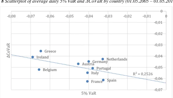
Figure 8 Scatterplot of average daily 5% VaR and ΔCoVaR by country

(01.05.2005 – 01.05.2015) ... 28

Figure 9 Average ΔCoVaR and VaR of 32 European banks

(01.05.2005 – 01.05.2015) ... 28

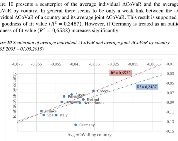
Figure 10 Scatterplot of average individual ΔCoVaR and average joint

ΔCoVaR by country (01.05.2005 – 01.05.2015 ... 30

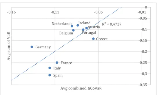
Figure 11 Scatterplot of average cumulative VaR and average comined

∆CoVaR by country (01.05.2005 – 01.05.2015) ... 31

Figure 12 Scatterplot of average correlation between institutions and average

combined ∆CoVaR by country (01.05.2005 – 01.05.2015) ... 32

Figure 13 Average cumulative VaR and average combined ∆CoVaR of all

(8)

Abbreviation Index

AR – Autoregressive

BIC – Bayesian information criterion CoES – Conditional expected shortfall CoVaR – Conditional value-at-risk DCC – Dynamic conditional correlation DIP – Distress insurance premium ES – Expected shortfall

GARCH – Generalized autoregressive conditional heteroskedasticity GJR GARCH – Glosten-Jagannathan-Runkle GARCH

MA – Moving average

MES – Marginal expected shortfall QML – Quasi-maximum likelihood SES – Systemic expected shortfall

SIFI – Systemically Important Financial Institution SRISK – Systemic risk measure

USD – United States dollar VaR – Value-at-risk

(9)

1

Introduction

In today’s globalized financial world the downfall of an individual financial institution can have severe consequences for both the financial system and the real economy. A prime example for such a scenario is the bankruptcy of Lehman Brothers, which struck the financial system heavily, led to several bail-outs of big financial institutions in the time after the event, and demonstrated the fragility of the whole financial system. Financial crises impose high costs for the society through the spillovers from the financial system to the real economy, which drops into a deep recession, and through the bailouts of big financial institutions with taxpayers’ money. Hence, the regulation of financial institutions and the managing of such systemic risks is a desirable goal for the society as a whole. In the light of the global financial crisis, researchers and policymakers have recognized the importance of managing systemic risk. Before the events of the global financial crisis, banking regulation was solely based on idiosyncratic risk measures, as implemented in the Basel I and Basel II accords. With the acknowledgement of the importance of systemic risk, regulation authorities are moving towards a new regulation framework, such as Basel III, that incorporates macro prudential policies which focus on the mitigation of systemic risks.

A rich literature on measuring systemic risk has evolved ever since the global financial crisis and numerous attempts have been made to apply the different systemic risk measures. One of the most famous systemic risk measures is 𝛥𝐶𝑜𝑉𝑎𝑅, introduced by Adrian and Brunnermeier (2008). 𝛥𝐶𝑜𝑉𝑎𝑅 measures the systemic risk contribution of an individual financial institution in the financial system. It is defined as the difference between the VaR of the system, conditional on an institution being in financial distress and the VaR of the system, conditional on this institution being in its benchmark state. Several studies, such as Cao (2013) and Girardi and Ergün (2013), have extended the 𝛥𝐶𝑜𝑉𝑎𝑅 measure and introduced new ways to calculate it. Cao (2013) introduced an extension to the original 𝛥𝐶𝑜𝑉𝑎𝑅 which allows for conditioning on several financial institutions being in distress at the same time. The extension is then applied to a French and Chinese banking panel. Girardi and Ergün (2013) proposed a way of calculating

𝛥𝐶𝑜𝑉𝑎𝑅 using multivariate GARCH models. Using their new methodology they measure the systemic risk contribution of US financial firms. This essay relies on key features from both studies as well as the original study by Adrian and Brunnermeier (2011).

As the epicenter of the global financial crisis, systemic risks in the financial system of the United States have been a main focus of research so far. However, little attempts have been made to analyze systemic risk contributions in the financial system of the European Monetary Union. Furthermore, the phenomenon of several institutions being simultaneously in financial distress has received little attention. Even though the collective failure of a group of banks is not just a theoretical construction but has been observed in practice, research on this phenomenon is very limited.

(10)

The aim of this essay is to analyze individual systemic risk contributions of 32 financial institutions from 10 different European Monetary Union countries, as well as their collective systemic risk contribution. Furthermore, the essay tries to identify the countries that are home to the most systemically risky financial institutions and to analyze the collective systemic risk contribution for cases of countrywide negative shocks to the associated banks. Extra attention is paid on the analysis of the collective systemic risk contribution of a group of banks and the underlying drivers of a group’s collective systemic risk contribution.

The remainder of the essay is structured in the following way. Chapter 2 provides an overview over existing research with respect to CoVaR and introduces the concept of systemic risk. The estimation and calculation methodology for 𝛥𝐶𝑜𝑉𝑎𝑅 is described in Chapter 3. Chapter 4 presents the data used for estimations and calculations. Empirical results for both the systemic risk contribution of individual banks and a group of banks are described in Chapter 5. The essay ends with a discussion and a summary in Chapter 6.

(11)

3

2

Related Literature and Theoretical Review

This chapter will consist of a review of previous research concerning the CoVaR measure as well as a theoretical discussion about systemic risk.

2.1

Previous Research on CoVaR

While systemic risk caught broad attention only after the global financial crisis, the literature on measuring and managing systemic risk is already rich and comprehensive. Several attempts have been made to categorize the different systemic risk approaches. Borri et al. (2012), for example, identify two main strands in the literature on systemic risk. The first one, referred to as network analysis, focuses on the interconnectedness of the entities in the financial system and thus is concerned with the joint distribution of losses. It assesses the impact of a failing network entity on the other network components’ viability. Further discussions regarding

network analysis lie beyond the scope of this essay. However, interested readers are referred to Martínez-Jaramillo et al. (2010) and Markose et al. (2010), as prime examples. The second strand, called micro-evidence approach measures systemic risk contribution of individual financial institutions. CoVaR, which is the measure of choice in this essay, is part of the micro-evidence approach strand. Thus focus in this essay is put on studies following this strand.

2.1.1

The first introduction of CoVaR

One of the most famous systemic risk measures is the so-called CoVaR measure, first introduced by Adrian and Brunnermeier in their paper CoVaR in 2008. It lead to a widespread application and analysis of their CoVaR measure. CoVaR is defined as the VaR of the financial system conditional on an institution 𝑖 being in financial distress (Adrian & Brunnermeier, 2011). The measure can be categorized as a tail measure and thus focuses on the co-dependence in the tails of equity returns between financial institutions or an institution and the financial system (Hansen, 2013). This is also emphasized by the name of the measure, chosen by the authors, in which “Co” stands for conditional, contagion or comovement (Adrian & Brunnermeier, 2011).

The objectives of their paper are to 1) measure the contribution of a financial institution to systemic risk which is achieved through the measure ∆CoVaR, and to 2) create a forward looking indicator based on firm characteristics to predict future risk contributions of financial institutions which they call “forward ∆CoVaR”. ∆CoVaR is defined as the difference between the 𝑞%-CoVaR of the system 𝑗 conditional on institution 𝑖 being in financial distress and the

(12)

∆𝐶𝑜𝑉𝑎𝑅_𝑞𝑗|𝑖 = 𝐶𝑜𝑉𝑎𝑅_𝑞𝑗|𝑋𝑖=𝑉𝑎𝑅𝑞 𝑖

− 𝐶𝑜𝑉𝑎𝑅_𝑞𝑗|𝑋𝑖=𝑀𝑒𝑑𝑖𝑎𝑛𝑖.

The authors define institution 𝑖’s state of financial distress as institution 𝑖’s equity returns being at their 1%-𝑉𝑎𝑅 level and its benchmark state as its equity returns being at their median level (50%-𝑉𝑎𝑅 level).

Adrian and Brunnermeier (2011) estimate both an unconditional version of the measure, which results in a constant CoVaR over time, and a conditional version of the measure, which varies over time. In order to estimate a time-varying conditional CoVaR measure, the authors include systemic state variables that model the changes in tail risk dependence over time. The vector of state variables contains the aggregate credit spread, the VIX as the implied equity return volatility, and the slope of the yield curve. For all of their estimations they use the so-called Quantile Regression which allows them to focus on the tails of equity returns. Their estimations are based on weekly equity return data of 1226 financial institutions, from 1986Q1 to 2010Q4, belonging to the four sectors: commercial banks, security broker-dealers (including investment banks), insurance companies and real estate companies.

The authors furthermore create the forward looking “forward ∆CoVaR” which is obtained by regressing the previously estimated ∆CoVaR on several firm characteristics such as size, market-beta, maturity mismatch, market-to-book ratio, and leverage. They find that a higher systemic risk contribution is related to a larger size, a higher leverage, and more maturity mismatch. Furthermore, “forward ∆CoVaR” is countercyclical, which means it is negatively correlated with the contemporaneous ∆CoVaR and thus captures the fact that systemic risk builds up in periods of tranquil market environments.

Another important finding by Adrian and Brunnermeier (2011) is the loose relation between conventional VaR and ∆CoVaR; that a high VaR does not automatically imply a high contribution to systemic risk. This implies that financial regulation based solely on idiosyncratic risks is not sufficient to protect against systemic risks. However, they do find a strong relation between an institution’s VaR and its systemic risk contribution ∆CoVaR in the time series dimension.

Since Adrian and Brunnermeier (2008) laid the foundation for the CoVaR measure a number of applications to different datasets and within different environments have emerged, such as in Arias, Mendoza, and Pérez-Reyna (2010), Borri et al. (2012), or Karkowska (2015). Assessments, extensions and customizations of the measure, such as in Cao (2013), Girardi and Ergün (2013), Karimalis and Nomikos (2014), Bernardi, Maruotti, and Petrella (2013), Benoit et al. (2013), and Mainik and Schaaning (2012), contributed to further developments of the CoVaR measure.

2.1.2

Multi-CoVaR and Shapley value

Cao (2013) in Multi-CoVaR and Shapley value: A Systemic Risk Measure, extends the basic CoVaR measure to a multivariate approach. By conditioning on more than one institution being in financial distress the Multi-CoVaR is able to measure the change in systemic risk when several institutions face financial difficulties at the same time.

(13)

5 The author follows a two-step procedure in order to calculate the contribution of a financial institution to systemic risk. First, the total systemic risk contribution for the case that all institutions in the system are in financial distress at the same time is calculated, which represents total systemic risk. Secondly, the systemic risk contribution of each institution is obtained by applying an allocation algorithm to the overall systemic risk. Thus, the definition of CoVaR slightly changes in the following way

∆𝐶𝑜𝑉𝑎𝑅_𝑞,𝑡1,…,𝑆 = 𝐶𝑜𝑉𝑎𝑅_𝑞,𝑡𝑟1≤𝑉𝑎𝑅𝑞1,…,𝑟𝑆≤𝑉𝑎𝑅𝑞𝑆

− 𝐶𝑜𝑉𝑎𝑅_𝑞,𝑡−𝛼𝜎𝑡1≤𝑟𝑡1≤𝛼𝜎𝑡1,…,−𝛼𝜎𝑡𝑆≤𝑟𝑡𝑆≤𝛼𝜎𝑡𝑆_,

where ∆𝐶𝑜𝑉𝑎𝑅_𝑞,𝑡1,…,𝑆 is the total systemic risk contribution of all institutions {1, … , 𝑆} at time 𝑡

and confidence level 𝑞, 𝐶𝑜𝑉𝑎𝑅_𝑞,𝑡𝑟 1_{≤𝑉𝑎𝑅}

𝑞1,…,𝑟𝑆≤𝑉𝑎𝑅𝑞𝑆

is the CoVaR of the system for all institutions being in financial distress, and 𝐶𝑜𝑉𝑎𝑅_𝑞,𝑡−𝛼𝜎𝑡1≤𝑟𝑡1≤𝛼𝜎𝑡1,…,−𝛼𝜎𝑡𝑆≤𝑟𝑡𝑆≤𝛼𝜎𝑡𝑆

is the CoVaR of the system for all institutions being in their benchmark state. Adrian and Brunnermeier (2011) define the benchmark state as institution 𝑖’s returns being at their median, while Cao (2013) defines the benchmark state as the institution’s returns being at an 𝛼 × 𝜎_𝑡-event around the mean, where 𝛼

is constant, and 𝜎𝑡 is the institution’s standard deviation at time 𝑡. Furthermore, while Adrian

and Brunnermeier (2011) only focus on a single institution being in financial distress, Cao (2013) calculates the total systemic risk contribution of all institutions in the system being in financial distress at the same time, and allocates the systemic risk contribution of a single institution in a second step.

In the second step Cao (2013) applies the so-called Shapley value methodology to the total systemic risk. The Shapley value was initially introduced for cooperative games where players create together one outcome for the whole group. For a single player the Shapley value is the expected marginal contribution to the outcome over the set of all permutations of players. It is a fair and efficient method to allocate the systemic risk contribution among the institutions and fulfills a set of favorable characteristics such as additivity1.

Cao (2013) also uses a different methodology compared to Adrian and Brunnermeier (2011). He starts by assuming an underlying multivariate student t-distribution for the returns of the system and each institution. Then, GARCH modeling for estimating the time-varying volatility of the returns and the DCC approach, introduced by Engle (2002), for estimating the time-varying correlations between the returns is used to obtain the joint distribution of the returns. For the VaR of each institution however, Cao (2013) uses a Bootstrap approach which does not depend on a distributional assumption and is thus less restrictive. Given the VaR of each institution and the joint distribution of the system’s and institutions’ returns, Cao (2013) solves numerically for the CoVaR value of the system conditional on the adverse state and the benchmark state, and obtains ∆CoVaR.

1_{For CoVaR, additivity means that the joint CoVaR of all institutions combined is equal to the sum of each} individual CoVaR-value. Thus the following must hold: 𝐶𝑜𝑉𝑎𝑅𝑞,𝑡1,…,𝑆= ∑𝑆𝑖=1𝐶𝑜𝑉𝑎𝑅𝑞,𝑡𝑖 .

(14)

The estimations are based on two panels, a French and a Chinese one, which consist of the five biggest institutions of each country for which weekly returns are extracted for the time between 19th_{April 2002 and 29}th_{January 2012 for the French panel, and between 27}th_{October 2006 and} 29th June 2012 for the Chinese panel. His results show that French banks are much more affected by the global and the European financial crisis than Chinese banks are, which indicates a lower global interconnectedness of the Chinese banks.

Another important finding is that while the Multi-CoVaR using Shapley values exhibits additivity, the Multi-CoVaR without Shapley values is smaller than the sum of the individual corresponding CoVaR’s.

2.1.3

CoVaR estimation using multivariate GARCH models

Another paper extending the CoVaR approach is Systemic risk measurement: Multivariate GARCH estimation of CoVaR by Girardi and Ergün (2013). In their paper the authors change the definition given by Adrian and Brunnermeier (2011) of an institution being exactly at its VaR level as its distress state to an institution being at most at its VaR level as its distress state, which is formulated as

Pr (𝑅𝑡𝑖 ≤ 𝐶𝑜𝑉𝑎𝑅𝑞,𝑡 𝑖|𝑗

|𝑅_𝑡𝑗 ≤ 𝑉𝑎𝑅_𝑞,𝑡𝑗 ) = 𝑞,

where 𝑅_𝑡𝑖 is the returns of the system 𝑖, 𝑅_𝑡𝑗 is the returns of institution 𝑗, 𝑉𝑎𝑅_𝑞,𝑡𝑗 is the VaR of institution 𝑗, and 𝑞 is the confidence level. This new definition also takes into account more severe outcomes than the VaR level and it opens up the possibility to back test the CoVaR measure as well as improves its consistency with respect to the dependence parameter between institution 𝑗 and the system 𝑖, as shown by Mainik and Schaanning (2012).

Similarly to Cao (2013), Girardi and Ergün (2013) define the benchmark case as a one-standard deviation around the mean return event. Furthermore, they also use a GARCH and DCC approach to obtain skewed-t and Gaussian joint distributions of the returns of the system and institution 𝑗, which are then used to solve numerically for CoVaR.

Their estimations and calculations are based on data of 74 US financial institutions with market value greater than 5bln USD for the time period between 26th June 2000 and 29th February 2008. The authors backtest their CoVaR results based on both the Gaussian and the skewed-t distribution using the Kupiec and the Christoffersen test. While the results based on the skewed-t disskewed-tribuskewed-tion assumpskewed-tion pass all skewed-tesskewed-ts, skewed-the resulskewed-ts from assuming a Gaussian disskewed-tribuskewed-tion exceed the confidence level in the unconditional coverage test. Furthermore, they find that the CoVaR estimates based on the skewed-t distribution are all higher than the estimates based on the Gaussian distributional assumption.

The authors also investigate the relation between firm characteristics and systemic risk contribution of an institution. Contrary to Adrian and Brunnermeier (2011), they do not find a strong relation between the VaR of an institution and its systemic risk contribution ∆𝐶𝑜𝑉𝑎𝑅 in the time series dimension, which implies that monitoring only the tail risk of an institution is not enough to predict its systemic risk contribution.

(15)

7

2.1.4

CoVaR estimation using Copula functions

Karimalis and Nomikos (2014) in Measuring systemic risk in the European banking sector: A Copula CoVaR approach also extend the CoVaR approach in the sense that they propose a new methodology for its calculation. In order to obtain the joint probability distribution of the system and an institution, the authors use so-called Copula functions. Copula functions can replicate the true multivariate joint distribution function using only the univariate marginal distribution of each series and a copula which describes the dependence between the two series.

Karimalis and Nomikos (2014) calculate the joint distributions using different types of copulas from different copula families, for both the definition of CoVaR given by Adrian and Brunnermeier (2011) (𝐶𝑜𝑉𝑎𝑅_𝑞𝑗|𝑋𝑖=𝑉𝑎𝑅𝑞𝑖) and for the definition given by Girardi and Ergün (2013) (𝐶𝑜𝑉𝑎𝑅_𝑞𝑗|𝑋

𝑖_{≤𝑉𝑎𝑅} 𝑞 𝑖

). Furthermore, they extend their calculations to obtain the conditional expected shortfall (CoES) of the system.

The authors base their estimations on return data of 42 European banks from 1st April 2002 to 31st December 2012. Similar to Girardi and Ergün (2013), they backtest their results and obtain similar results concerning the Gaussian and the skewed-t distribution.

Furthermore, the authors suggest ways for stress testing using their copula approach. These ways include changing the marginal distributional assumptions, changing the copula functions, or changing the dependence structure between the series.

Karimalis and Nomikos (2014) also analyze the relation between VaR and ∆CoVaR and come to the conclusion that depending on the definition of the benchmark case, the link between VaR and ∆CoVaR is strong if the benchmark case is defined according to Adrian and Brunnermeier (2011), and weak if the benchmark case is defined as in Girardi and Ergün (2013). Following the work of Adrian and Brunnermeier (2011), Karimalis and Nomikos (2014) also assess the influence of common market factors as well as firm characteristics on the systemic risk contribution of an institution and receive similar results, namely that size, leverage and equity beta are key drivers of systemic risk.

2.1.5

Systemic risk measures in comparison

Benoit et al. (2013) in A Theoretical and Empirical Comparison of Systemic Risk Measures

analyze several systemic risk measures, including CoVaR, both theoretically and empirically. For their analysis they focus on the three systemic risk measures: MES, SRISK, and ∆CoVaR. Through their theoretical assessment of ∆CoVaR, the authors come to the conclusion that, given the definition of ∆CoVaR by Adrian and Brunnermeier (2011), the measure is simply a linear projection of the institution’s VaR and thus can be expressed as

(16)

where 𝛾𝑖𝑡 = 𝜌𝑖𝑡𝜎𝑚𝑡

𝜎𝑖𝑡 is the linear projection coefficient of the market return on the firm return, 𝜌_𝑖𝑡 is the correlation between the market and the firm at time 𝑡, 𝜎_𝑚𝑡 is the volatility of the market at time 𝑡, and 𝜎𝑖𝑡 is the volatility of the firm at time 𝑡. Benoit et al. (2013) find that, due

to the scaling nature of 𝛾_𝑖𝑡, ranking the institutions by their VaR and by their ∆CoVaR may lead to different results. However, they further find that for an individual institution, forecasting VaR is sufficient to predict the evolution of its systemic risk contribution ∆CoVaR.

The authors also compare the ranking of the institutions’ systemic risk contribution as measured by their MES and ∆CoVaR, and conclude that the rankings may not be equivalent. However, they also find that the higher the correlation between an institution’s returns and the system’s returns, the more likely it is that MES and ∆CoVaR lead to the same systemic risk contribution ranking. Thus, even though the systemic risk measures have differing definitions, under certain conditions they will produce the same output. For the relation between SRISK and ∆CoVaR, the authors find that only under certain restrictive conditions, namely a high leverage of the bank and a high correlation of the bank’s returns with the system’s returns, the two measures will lead to equivalent results.

Besides their theoretical analysis of the three systemic risk measures, Benoit et al. (2013) also conduct an empirical comparison of the measures. They base their results on data of 94 US financial firms with market capitalization above 5 bn. USD for the period between 3rd January 2000 and 31st_{December 2010. The ∆CoVaR outputs that are used for the assessment are} obtained through a Quantile Regression. The authors conduct their comparison by ranking the ten so-called SIFI’s (systemically important financial institution) as the institutions with the highest systemic risk contribution according to the three measures. They find that the different systemic risk measures lead to different identification of SIFI’s and report little overlap between the identified SIFI’s. In addition, their empirical results confirm what has been concluded previously on a theoretical basis, namely that there is only a weak link between the VaR of an institution and its systemic risk contribution ∆CoVaR in the cross-sectional dimension, but a strong relation in the time-series dimension.

2.1.6

Summary and limitations of CoVaR

The rich literature on CoVaR, including applications of the measure, in-depth analysis of its properties, and numerous extensions to the measure, show that the measure indeed makes an important contribution to the understanding, measuring, and managing of systemic risk. It has been shown that regulating financial institutions according to their idiosyncratic risk measured by VaR is not sufficient, given the loose link between its VaR level and its actual contribution to systemic risk measured by ∆CoVaR. Thus ∆CoVaR can be considered a useful tool in the process of identifying and managing systemic risks.

However, there are also limitations to the CoVaR approach. While in the cross-sectional dimension there is only a weak relation between an institution’s VaR and its ∆CoVaR, in the

(17)

9 time-series dimension the evolution of the VaR of an institution resembles its ∆CoVaR evolution very closely. Thus it can be argued that ∆CoVaR does not capture the multiple facets of systemic risk and hence adds only little additional information beyond its idiosyncratic VaR measure (Benoit et al., 2013). Furthermore, systemic risk is characterized by a multitude of key features encompassed in it, of which ∆CoVaR only captures a small amount and is silent about features such as spillover effects to the real economy or the path systemic risk takes when spreading across a network.

2.2

Systemic Risk

So far, no consensus has been reached by researchers regarding the definition of systemic risk but rather a multitude of systemic risk definitions have evolved (Smaga, 2014). The European Central Bank (2009), for example, defines systemic risk as “the risk that financial instability becomes so widespread that it impairs the functioning of a financial system to the point where economic growth and welfare suffer materially“ (p. 134). While the definition by the European Central Bank is rather vague, Bisias et al. (2013) list in their survey of systemic risk measures more precise characteristics on which other authors have focused on for their definition of systemic risk. The list includes aspects such as imbalances, spillover effects to the real economy, asset bubbles, correlated exposures of banks, feedback reactions of financial institutions, contagion, information disturbances, and negative externalities.

Smaga (2014) analyzes definitions of systemic risk in the literature with respect to the most common features associated with systemic risk. His analysis takes definitions from 55 different papers, studies and articles into consideration, dating from 1995 to 2014, and he summarizes his results as follows:

- The transmission of shocks between the interconnected institutions of the financial system, which eventually leads to possible adverse results for the real economy, is a key feature of systemic risk.

- In a large part of the literature it is highlighted that systemic risk affects the whole financial system or a majority of the financial institutions, and interferes with the operations and the purpose of the system, e.g. financial intermediation. However, the loss of confidence in the financial system that systemic risk causes is considered only by a small group of authors.

- The first definitions of systemic risk were introduced between 1995 and the time of the global financial crisis and focused mainly on the contagion effect and the wide range of affection of this occurrence. After the financial crisis the number of research on systemic risk increased dramatically and with it the number of definitions of systemic risk. Furthermore, part of the emphasis was shifted towards the disruption of the features of the financial system and the negative spillover effects this causes for the real economy. Systemic risk can be summarized as a complex phenomenon that manifests itself through a wide range of different characteristics and affects the entire financial system which yields adverse results for both the financial system and the real economy through spill-over effects.

(18)

The multitude of definitions of systemic risk is a reflection of the undoubtable complexity of the phenomenon, and consensus on a single all-encompassing definition might never be reached. Naturally, the high number of different definitions results in a similarly high number of different systemic risk measures, and just as the various definitions emphasize on different aspects of systemic risk so are the systemic risk measures based on different aspects of the phenomenon.

The main focus of this essay lies on ∆CoVaR to measure systemic risk. However, as mentioned above there exists a long list of different systemic risk measures. A selection of systemic risk measures are briefly introduced in Appendix A of the essay.

(19)

11

3

Methodology

As described in Section 2, several extensions of the ∆CoVaR measure with respect to the methodology have been developed. In this essay, the methodology is based on the work of Cao (2013) and Girardi and Ergün (2013), who use a GARCH-DCC approach to model the time-varying joint distribution of the system and a single institution, and calculate the systemic risk contribution of one or more institutions. The advantage of a GARCH-DCC approach, compared to a quantile regression, which Adrian and Brunnermeier (2011) use to calculate ∆CoVaR, lies in the feature that the GARCH-DCC approach allows to take into account time-varying linkages between the system and one or more institutions without having to rely on systemic state variables (Girardi & Ergün, 2013).

3.1

VaR as a starting point

Recall that VaR is defined as the 𝑞-quantile of the return distribution and thus can be formulated in terms of returns in the following way,

Pr(𝑟_𝑡≤ 𝑉𝑎𝑅_𝑡𝑞) = 𝑞, (1)

where 𝑟_𝑡 is the return at time 𝑡, and 𝑉𝑎𝑅_𝑖,𝑡𝑞 is the 𝑞-quantile of the returns 𝑟_𝑡 at time 𝑡. This implies that VaR can also be written as the upper boundary of an integral in the following formulation,

∫ 𝑝𝑑𝑓𝑡(𝑟𝑡) 𝑑𝑟𝑡 𝑉𝑎𝑅_𝑡𝑞

−∞

= 𝑞, (2)

where 𝑝𝑑𝑓_𝑡(𝑟_𝑡) is the probability density function of the returns at time 𝑡.

3.2

Definition of CoVaR

Recall from the previous section, that CoVaR is defined as the VaR of the financial system conditional on an institution 𝑖 being at its 𝑉𝑎𝑅𝑞_{-level, which represents financial distress for}

this institution. By changing the definition of CoVaR to the VaR of the system conditional on an institution 𝑖 being at most at its 𝑉𝑎𝑅𝑞_{-level, the CoVaR measure exhibits favorable}

(20)

that only with the latter definition of CoVaR, the measure is an increasing continuous function of the dependence parameter between the system and institution 𝑖. Furthermore, the definition can be extended to account for 𝑁 institutions being in financial distress at the same time as introduced by Cao (2013). Thus following the definition of CoVaR by Girardi and Ergün (2013) and Cao (2013), in this essay, CoVaR for the general case of 𝑁 institutions being at most at their 𝑉𝑎𝑅𝑞-level is defined as the 𝑞-quantile of the following conditional distribution,

Pr(𝑟_𝑡𝑆 ≤ 𝐶𝑜𝑉𝑎𝑅_𝑞,𝑡𝑆|1,…,𝑁|𝑟_𝑡1 ≤ 𝑉𝑎𝑅_𝑞,𝑡1 , … , 𝑟_𝑡𝑁 ≤ 𝑉𝑎𝑅_𝑞,𝑡𝑁 ) = 𝑞, (3) where 𝑟𝑡𝑆 is the return of the system 𝑆 at time 𝑡, 𝑟𝑡𝑖 is the return of institution 𝑖 at time 𝑡, 𝐶𝑜𝑉𝑎𝑅_𝑞,𝑡𝑆|1,…,𝑁 is the CoVaR measure conditional on institutions {1, … , 𝑁} being in distress, and

𝑉𝑎𝑅_𝑞,𝑡𝑖 _{is the VaR of institution}_𝑖_{at time}_𝑡_{at confidence level}_𝑞_{. Following Girardi and Ergün}

(2013), the CoVaR measure of the system conditional on 𝑁 institutions being in their benchmark state 𝑏1,…,𝑁_{, is in this essay defined as the one standard-deviation around the mean}

event 𝜇_𝑡𝑖 − 𝜎_𝑡𝑖 ≤ 𝑟_𝑡𝑖 ≤ 𝜇_𝑡𝑖 + 𝜎_𝑡𝑖, where 𝜇_𝑡𝑖 is the mean of institution 𝑖 at time 𝑡 and 𝜎_𝑡𝑖 is the standard deviation of institution 𝑖 at time 𝑡. Given both the CoVaR measure for the distress state and the CoVaR measure for the benchmark state, the combined systemic risk contribution ∆CoVaR of 𝑁 institutions can be expressed as

∆𝐶𝑜𝑉𝑎𝑅_𝑞,𝑡𝑆|1,…,𝑁 = 𝐶𝑜𝑉𝑎𝑅_𝑞,𝑡𝑆|1,…,𝑁− 𝐶𝑜𝑉𝑎𝑅_𝑞,𝑡𝑆|𝑏1,…,𝑁, (4) where 𝐶𝑜𝑉𝑎𝑅_𝑞,𝑡𝑆|1,…,𝑁 is the CoVaR measure of the system conditional on institutions {1, … , 𝑁}

being in financial distress, and 𝐶𝑜𝑉𝑎𝑅_𝑞,𝑡𝑆|𝑏1,…,𝑁 is the CoVaR measure of the system conditional on institutions {1, … , 𝑁} being in their benchmark state.

3.3

Calculations steps of the CoVaR measure

In order to increase the traceability of the calculations needed to obtain the ∆CoVaR measure, the calculation procedure is divided into three steps.

3.3.1

Step 1: Calculation of individual VaR

In a first step, a distributional assumption about the returns of the institutions in the system and the system itself has to be made. For the returns an underlying student t-distribution is assumed which accounts for fatter tails than a normal distribution, a well-known stylized fact of financial returns. Hence, the returns are defined as

𝑟_𝑡𝑖_~𝑡

𝜈(𝜇𝑡𝑖, 𝜎𝑖,𝑡2),

where 𝜇_𝑡𝑖_{is the mean,}_𝜎

𝑖,𝑡2 is the variance, and 𝜈 are the degrees of freedom of the student

t-distribution. By assuming an underlying student t-distribution for the returns, the VaR for each institution, and the system itself, can be calculated using the following formula

(21)

13

𝑉𝑎𝑅_𝑡𝑞(𝑟_𝑡𝑖) = 𝜇_𝑡𝑖 + √𝜈 − 2 𝜈 𝜎𝑡+1

𝑖 _𝑡

𝑞,𝜈, (5)

where 𝑡_𝑞,𝜈 is the 𝑞-quantile of the student t-distribution with 𝜈 degrees of freedom (Nilsson, 2015).

In order to obtain the inputs required to calculate the VaR for each institution and the system, a univariate GJR GARCH(1,1) model is estimated. The GJR GARCH model, first introduced by Glosten, Jagannathan and Runkle (1993), accounts for the so-called leverage effect which is commonly observed for financial data. The leverage effect usually refers to negative shocks having a bigger effect on changes in volatility than positive shocks. Here, the variance equation of the GJR GARCH model, in the formulation introduced by Ding, Granger and Engle (1993), is being used. The mean equation of the model is specified in the following way

𝑟_𝑡𝑖 _{= 𝑎} 0+ ∑ 𝑎𝑗𝑟𝑡−𝑗𝑖 + 𝜀𝑡𝑖 + ∑ 𝑏𝑘𝜀𝑡−𝑘𝑖 𝑞 𝑘=1 𝑝 𝑗=1 , (6) with 𝜀_𝑡𝑖 = 𝜎_𝑡𝑣_𝑡 and 𝑣_𝑡~𝑖𝑖𝑑(0,1),

where 𝑎0 is an intercept term, 𝑎𝑗𝑟𝑡−𝑗𝑖 is the autoregressive component, 𝑏𝑘𝜀𝑡−𝑘𝑖 is the moving

average component, and 𝜀_𝑡𝑖 are the error terms.

The number of lags in the AR part, denoted by 𝑝 in the sum, and the number of lags in the MA part, denoted by 𝑞 in the sum, in Equation (6) are determined by the Bayesian Information Criterion (BIC).

The variance equation of the model is specified as

𝜎_𝑡𝛿 = 𝜔 + 𝛼1(|𝜀𝑡−1𝑖 | − 𝛾1𝜀𝑡−1𝑖 ) 𝛿

+ 𝛽1𝜎𝑡−1𝛿 , (7)

where 𝛼1 measures the size of the impact of a shock on volatility, 𝛽1 measures the persistence

of shocks on volatility, 𝛿 indicates if the variance equation represents the conditional variance or the conditional standard deviation, and 𝛾1 captures the leverage effect. For 𝛾1 > 0, negative

shocks increase the conditional variance more than positive shocks and vice versa for 𝛾₁ < 0. For 𝛾1 = 0, the GJR GARCH model boils down to a standard symmetric GARCH model.

The model is estimated using the quasi-maximum likelihood estimation method, which yields estimates for the conditional mean 𝜇𝑡, the conditional variance 𝜎𝑡2, and the degrees of freedom 𝜈. These estimates for each institution and the system are then used to calculate its VaR using the VaR-formula in Equation (5).

(22)

3.3.2

Step 2: Estimation of the joint probability density function

For the estimation of the correlations between the system’s returns and the returns of one or more institutions, the dynamic conditional correlation approach (DCC) by Engle (2002) is used. In order to calculate the CoVaR measure, another distributional assumption for the joint distribution of the system’s returns and the 𝑁 institutions’ returns has to be made. To take into account the well-known fact of fat tails of financial data, a multivariate student t-distribution is assumed for the joint distribution

( 𝑟_𝑡𝑆 𝑟_𝑡1 ⋮ 𝑟_𝑡𝑁 ) ~𝑡_𝜈 ( ( 𝜇_𝑡𝑆 𝜇_𝑡1 ⋮ 𝜇_𝑡𝑁 ) , ( 𝜎_𝑆,𝑡2 𝜌𝑆1,𝑡𝜎𝑆,𝑡𝜎1,𝑡 ⋯ 𝜌𝑆𝑁,𝑡𝜎𝑆,𝑡𝜎𝑁,𝑡 𝜌_1𝑆,𝑡𝜎_1,𝑡𝜎_𝑆,𝑡 𝜎_1,𝑡2 ⋯ 𝜌_1𝑁,𝑡𝜎_1,𝑡𝜎_𝑁,𝑡 ⋮ ⋮ ⋱ ⋮ 𝜌_{𝑁𝑆,𝑡}𝜎_𝑁,𝑡𝜎_𝑆,𝑡 𝜌_𝑁1,𝑡𝜎_𝑁,𝑡𝜎_1,𝑡 … 𝜎_𝑁,𝑡2 )₎ , where 𝑟_𝑡 = (𝑟_𝑡𝑆, 𝑟_𝑡1_{, … , 𝑟}

𝑡𝑁)′ is the (𝑁 + 1 × 1) vector of returns, 𝜇𝑡 = (𝜇𝑡𝑆, 𝜇𝑡1, … , 𝜇𝑡𝑁)′ is the (𝑁 + 1 × 1) vector of conditional means, and Σ𝑡 is the (𝑁 + 1 × 𝑁 + 1) conditional

covariance matrix, 𝜎_𝑖,𝑡 is the conditional standard deviation of 𝑖, and 𝜌_{𝑖𝑗,𝑡} is the conditional correlation between 𝑖 and 𝑗.

The correlation coefficients defined as the (𝑁 + 1 × 𝑁 + 1) matrix of conditional correlations can be denoted as 𝑅𝑡 = 𝑑𝑖𝑎𝑔(Σ𝑡)−1 2⁄ Σ𝑡𝑑𝑖𝑎𝑔(Σ𝑡)−1 2⁄ = 𝜌𝑖𝑗,𝑡. Following Engle (2002), the

conditional correlation matrix is estimated by the following model:

𝑅_𝑡 = 𝑑𝑖𝑎𝑔(Q_𝑡)−1 2⁄ _Q

𝑡𝑑𝑖𝑎𝑔(Q𝑡)−1 2⁄ , (8)

where

Q_𝑡 = (1 − 𝛿₁− 𝛿₂)𝑄̅ + 𝛿₁(𝜀_𝑡−1∗ _𝜀

𝑡−1∗ ′) + 𝛿2𝑄𝑡−1. (9)

𝑄̅ is the unconditional covariance matrix of the standardized residuals 𝜀_𝑡∗ _{= 𝜀}

𝑡× 𝑑𝑖𝑎𝑔(Q𝑡)−1 2⁄ ,

and 𝛿₁ and 𝛿₂ are non-negative scalars that fulfill the following condition of stationarity 𝛿₁+ 𝛿2 < 1.

The DCC approach follows a two-step procedure. For both steps the QML estimation method is used. In the first step, the volatility part of the joint student t-distribution from above is estimated. For this purpose the respective underlying GJR GARCH (1,1) model from the previous step is fitted to each institution’s return series. In addition, the shape parameter given by the degrees of freedom 𝜈 is estimated for the joint student t-distribution. In the second step, the correlation part is estimated using the model described in Equation (8) and (9), with the estimates from step one serving as inputs. Thus, given the estimates from the DCC approach the conditional covariance matrix Σ𝑡 can be specified entirely.

Given the estimates for the conditional mean vector 𝜇_𝑡 = (𝜇_𝑡𝑆, 𝜇_𝑡1_{, … , 𝜇}

𝑡𝑁)′, the conditional

covariance matrix Σ𝑡, and the degrees of freedom 𝜈 of the multivariate student t-distribution,

(23)

15

3.3.3

Step 3: Calculating CoVaR

After obtaining all the inputs needed to calculate CoVaR, the parameters are used in the following equations to obtain the systemic risk measure.

Recall the definition of CoVaR from above,

Pr(𝑟_𝑡𝑆 ≤ 𝐶𝑜𝑉𝑎𝑅_𝑞,𝑡𝑆|1,…,𝑁|𝑟_𝑡1 _{≤ 𝑉𝑎𝑅}

𝑞,𝑡1 , … , 𝑟𝑡𝑁≤ 𝑉𝑎𝑅𝑞,𝑡𝑁 ) = 𝑞. (10)

By means of conditional probabilities, the above definition can be reformulated as

Pr(𝑟_𝑡𝑆 ≤ 𝐶𝑜𝑉𝑎𝑅_𝑞,𝑡𝑆|1,…,𝑁∩ 𝑟_𝑡1 _{≤ 𝑉𝑎𝑅} 𝑞,𝑡 1 _{, … , 𝑟} 𝑡𝑁 ≤ 𝑉𝑎𝑅𝑞,𝑡𝑁 ) Pr(𝑟_𝑡1 _{≤ 𝑉𝑎𝑅} 𝑞,𝑡 1 _{, … , 𝑟} 𝑡𝑁 ≤ 𝑉𝑎𝑅𝑞,𝑡𝑁 ) = 𝑞. (11)

Given the VaR estimates from Step 1 and the joint probability density function of the returns obtained in Step 2, the denominator Pr(𝑟_𝑡1 ≤ 𝑉𝑎𝑅_𝑞,𝑡1 , … , 𝑟_𝑡𝑁 ≤ 𝑉𝑎𝑅_𝑞,𝑡𝑁 ) of the above equation can easily be solved, yielding a joint probability 𝑞𝑑

∫ … ∫ 𝑝𝑑𝑓_𝑡(𝑟_𝑡1_{, … , 𝑟} 𝑡𝑁) 𝑑𝑟𝑡1⋯ 𝑑𝑟𝑡𝑁 𝑉𝑎𝑅𝑞,𝑡𝑁 −∞ 𝑉𝑎𝑅𝑞,𝑡1 −∞ = 𝑞_𝑑. (12)

Thus, by plugging in the result from Equation (12) and through simple rearrangements of terms, Equation (11) becomes

Pr(𝑟_𝑡𝑆 ≤ 𝐶𝑜𝑉𝑎𝑅_𝑞,𝑡𝑆|1,…,𝑁∩ 𝑟_𝑡1 ≤ 𝑉𝑎𝑅1_𝑞,𝑡, … , 𝑟_𝑡𝑁≤ 𝑉𝑎𝑅_𝑞,𝑡𝑁 ) = 𝑞 × 𝑞_𝑑. (13) In the same fashion as the denominator in Equation (11) has been reformulated, Equation (13) can be reformulated the following way,

∫ ∫ … ∫ 𝑝𝑑𝑓𝑡(𝑟𝑡𝑆, 𝑟𝑡1, … , 𝑟𝑡𝑁)𝑑𝑟𝑡𝑆𝑑𝑟𝑡1⋯ 𝑑𝑟𝑡𝑁 𝑉𝑎𝑅𝑞,𝑡𝑁 −∞ 𝑉𝑎𝑅𝑞,𝑡1 −∞ 𝐶𝑜𝑉𝑎𝑅_𝑞,𝑡𝑆|1,…,𝑁 −∞ = 𝑞 × 𝑞𝑑. (14)

Since all other parameters are given, Equation (14) can be solved numerically with respect to

𝐶𝑜𝑉𝑎𝑅_𝑞,𝑡𝑆|1,…,𝑁 for each time period 𝑡, yielding the CoVaR measure conditional on 𝑁 institutions being in financial distress.

In order to calculate the combined systemic risk contribution of the 𝑁 institutions, a benchmark case of the CoVaR measure is needed. Following Girardi and Ergün (2013) and Cao (2013), the CoVaR for the benchmark state is defined as

Pr (𝑟_𝑡𝑆≤ 𝐶𝑜𝑉𝑎𝑅_𝑞,𝑡𝑆|𝑏1,…,𝑁| 𝜇_𝑡1_{− 𝜎}

𝑡1≤ 𝑟𝑡1≤ 𝜇𝑡1+ 𝜎𝑡1, … , 𝜇𝑡𝑁− 𝜎𝑡𝑁 ≤ 𝑟𝑡𝑁 ≤ 𝜇𝑡𝑁+ 𝜎𝑡𝑁) = 𝑞, (15)

where 𝜇_𝑡𝑖 − 𝜎_𝑡𝑖 ≤ 𝑟_𝑡𝑖 ≤ 𝜇_𝑡𝑖 + 𝜎_𝑡𝑖 is the one standard-deviation event around the mean.

Again, as in the distress case, Equation (15) can be reformulated by means of conditional probabilities,

(24)

Pr (𝑟𝑡𝑆≤ 𝐶𝑜𝑉𝑎𝑅𝑞,𝑡 𝑆|𝑏1,…,𝑁 ∩ 𝜇𝑡1− 𝜎𝑡1 ≤ 𝑟𝑡1≤ 𝜇𝑡1+ 𝜎𝑡1, … , 𝜇𝑡𝑁− 𝜎𝑡𝑁≤ 𝑟𝑡𝑁≤ 𝜇𝑡𝑁+ 𝜎𝑡𝑁) Pr(𝜇_𝑡1_{− 𝜎} 𝑡1 ≤ 𝑟𝑡1≤ 𝜇𝑡1+ 𝜎𝑡1, … , 𝜇𝑁𝑡 − 𝜎𝑡𝑁≤ 𝑟𝑡𝑁≤ 𝜇𝑡𝑁+ 𝜎𝑡𝑁) = 𝑞. (16)

For the denominator in Equation (16), the joint probability 𝑝_𝑑 in the benchmark case can be obtained by solving the following equation

∫ … ∫ 𝑝𝑑𝑓_𝑡(𝑟_𝑡1_{, … , 𝑟} 𝑡𝑁) 𝑑𝑟𝑡1⋯ 𝑑𝑟𝑡𝑁 𝜇_𝑡𝑁+𝜎_𝑡𝑁 𝜇_𝑡𝑁−𝜎_𝑡𝑁 𝜇_𝑡1+𝜎_𝑡1 𝜇_𝑡1−𝜎_𝑡1 = 𝑝_𝑑. (17)

Plugging in the result from Equation (17) into Equation (16) and rearranging terms yields

Pr (𝑟𝑡𝑆≤ 𝐶𝑜𝑉𝑎𝑅𝑞,𝑡

𝑆|𝑏1,…,𝑁

∩ 𝜇𝑡1− 𝜎𝑡1≤ 𝑟𝑡1≤ 𝜇𝑡1+ 𝜎𝑡1, … , 𝜇𝑡𝑁− 𝜎𝑡𝑁≤ 𝑟𝑡𝑁≤ 𝜇𝑡𝑁+ 𝜎𝑡𝑁) = 𝑞 × 𝑝𝑑. (18)

Given all other parameters, by rewriting Equation (18) in terms of a multiple integral and a probability density function, it is once again possible to solve numerically for 𝐶𝑜𝑉𝑎𝑅_𝑞,𝑡𝑆|𝑏1,…,𝑁

using the following formula,

∫ ∫ … ∫ 𝑝𝑑𝑓_𝑡(𝑟_𝑡𝑆_{, 𝑟} 𝑡1, … , 𝑟𝑡𝑁)𝑑𝑟𝑡𝑆𝑑𝑟𝑡1⋯ 𝑑𝑟𝑡𝑁 𝜇_𝑡𝑁+𝜎_𝑡𝑁 𝜇𝑡𝑁−𝜎𝑡𝑁 𝜇_𝑡1+𝜎_𝑡1 𝜇𝑡1−𝜎𝑡1 𝐶𝑜𝑉𝑎𝑅_𝑞,𝑡𝑆|𝑏1,…,𝑁 −∞ = 𝑞 × 𝑝_𝑑. (19)

Given the CoVaR measure for the benchmark and the distress state, the combined systemic risk contribution of 𝑁 financial institutions can be calculated by taking the difference of the two CoVaR measures

∆𝐶𝑜𝑉𝑎𝑅_𝑞,𝑡𝑆|1,…,𝑁 = 𝐶𝑜𝑉𝑎𝑅_𝑞,𝑡𝑆|1,…,𝑁− 𝐶𝑜𝑉𝑎𝑅_𝑞,𝑡𝑆|𝑏1,…,𝑁. (20) The above described calculations and estimations apply both for the case of measuring the combined systemic risk contribution of several financial institutions, and for the case of measuring the systemic risk contribution of an individual institution. In the latter case, some of the estimations and equations can be simplified. Appendix B provides information about the estimations and calculations used for measuring the systemic risk contribution of an individual institution.

(25)

17

4

Data

For the estimations and calculations in this essay, stock market data of 32 European banks from 10 different Eurozone countries are used. The data consists of daily stock prices covering a time period of 10 years from 1st May 2005 to 1st May 2015 and has been obtained through Datastream.

A complete overview of all included banks can be found in Appendix C. Table 1 provides an overview of the number of banks per country included in the sample. The number of countries that participated in the European Monetary Union over the whole sample period is limited to a total of 12 countries. These are the 11 member states that founded the union in 1999 and Greece, which joined the union in 2001. Finland and Luxembourg however have not been included in the sample due to the lack of data on listed banks from the respective countries.

Table 1 Number of banks per country

Country Austria Belgium France Germany Greece Ireland Italy Netherlands Portugal Spain No. of

Banks 2 2 4 4 4 2 5 2 2 5

Percentage returns for each institution have been generated using the following formula,

𝑟_𝑡𝑖 ₌𝑃𝑡 𝑖 _{− 𝑃}

𝑡−1𝑖 𝑃_𝑡−1𝑖 ,

where 𝑟_𝑡𝑖 is the return of institution 𝑖 at time 𝑡, 𝑃_𝑡𝑖 is the closing price of institution 𝑖 at time 𝑡, and 𝑃_𝑡−1𝑖 is the closing price of institution 𝑖 at time 𝑡 − 1. Using returns instead of prices brings the advantage of a unit free measure with it.

As a representation of the financial system, a market-value-weighted return index of the 32 European banks has been created, using the following formula,

𝑟_𝑡𝑆 = ∑ 𝑤_𝑡𝑖𝑟_𝑡𝑖 32 𝑖=1 , where 𝑤_𝑡𝑖 = 𝑀𝑉𝑡 𝑖 ∑32_𝑖=1𝑀𝑉_𝑡𝑖 .

𝑤_𝑡𝑖 is the weight of institution 𝑖 at time 𝑡, 𝑀𝑉_𝑡𝑖 is the market value of institution 𝑖 at time 𝑡,

∑32 𝑀𝑉_𝑡𝑖

𝑖=1 is the total market value of all 32 institutions at time 𝑡, and 𝑟𝑡𝑆 is the

(26)

Following the hypothesis of efficient financial markets, using publicly available stock prices has the advantage of taking all available information into account, as they are reflected by the prices. While these prices are sufficient for measuring the historical and contemporaneous systemic risk contribution of an institution, their use in forecasting future systemic risk contributions of an individual bank is limited. In order to forecast the systemic risk contribution of an institution, information regarding firm specific characteristics are needed. Unfortunately, this kind of information is only available to the regulation authorities, and not to the public.

(27)

19

5

Empirical Results

In this chapter, the results and findings from the estimations and calculations will be presented. Given the sample size, the output will be aggregated on a country level using averages. However, the individual estimation output for all 32 financial institutions in the sample can be found in Appendix E. First, summary statistics concerning the dataset will be presented. Second, a summary of the estimation parameters of the GARCH and the DCC model, as well as an overview of the VaR of the financial institutions will be given. Third, the time-varying ∆CoVaR outputs will be presented and analyzed. Fourth, a worst-case scenario by country is presented, where CoVaR is calculated conditional on all financial institutions of a certain country being in distress at the same time.

5.1

Summary statistics

Table 2 below gives an overview of the characteristics of the return data used for estimations and calculations. Average daily returns for the period 1st May 2005 to 1st May 2015 were highest for Belgian, French and Austrian banks. The lowest average daily returns are exhibited by Greek, Irish, and Portuguese financial institutions. Average standard deviation, which can be seen as a proxy for risk, was highest for banks from Belgium, Ireland and Greece. Spanish, Dutch and Portuguese financial institutions experienced the lowest volatility, as measured by the average standard deviation. Another interesting characteristic is the average kurtosis of the return data. Banks from all 10 European countries considered in the sample show an average kurtosis more than two times larger than three. In fact, none of the returns series of the financial institutions exhibit a kurtosis lower than five, as Appendix D shows. Since the kurtosis of a normal distribution is three, these results imply that estimations of CoVaR based on the assumption of a normal distribution may be incorrect as they do not take into account the fatter tails of the actual underlying distribution. This supports the assumption of an underlying student t-distribution.

(28)

Table 2 Summary statistics of return data aggregated at country level (01.05.2005 – 01.05.2015)

Country Mean (%) St. Dev (%) Max (%) Min (%) Kurtosis Skewness Austria 0,0244 3,1102 18,6160 -21,3831 8,9038 0,1073 Belgium 0,0870 5,9719 74,9533 -30,5980 25,2728 1,6526 France 0,0388 2,9197 27,4777 -16,0813 13,0472 0,7863 Germany -0,0104 3,0203 31,3208 -22,2003 20,9547 0,7374 Greece -0,0683 4,7344 29,4866 -28,3954 10,2808 0,5149 Ireland -0,0189 5,2441 45,7898 -56,6888 19,4301 0,5736 Italy -0,0140 2,7802 18,6175 -16,8706 8,7257 0,2082 Netherlands 0,0114 2,4234 20,8717 -18,3403 13,2168 0,4646 Portugal -0,0156 2,6236 26,9663 -14,0615 13,8034 1,0392 Spain 0,0136 2,2008 19,7384 -10,9791 9,9640 0,7131

5.2

Estimation output GJR GARCH, DCC, and VaR

5.2.1

Estimation output

In order to estimate the individual VaR of each financial institution, an underlying student t-distribution is assumed. The underlying t-distribution can be defined by its mean, its variance and its degrees of freedom. By fitting a GJR GARCH model to each return series, the necessary inputs for the underlying distribution are obtained. Summary statistics of the conditional mean, the conditional variance, and the dynamic conditional correlations, all aggregated at country level, are presented in Table 3.

The estimation results in the first column of Table 3 show that the fitted models for banks from France, Belgium, Austria, and Spain yield a positive average conditional mean, with French, Belgian, and Austrian banks exhibiting the highest average conditional mean. A positive conditional mean implies that the return distributions for these banks are shifted to the right compared to a standard student t-distribution, which is centralized around zero. In contrast, the fitted GJR GARCH models for financial institutions from Portugal, Italy, Ireland, Germany, the Netherlands, and Greece, yield negative average conditional means, suggesting that their return distributions are located to the left of zero. Among the financial institutions whose return distribution is shifted to the left, Portuguese, Italian, and Irish banks’ return distributions are located the furthest from zero since they exhibit the lowest average conditional means. The estimation results of the average conditional mean, as presented in the first column of Table 3, show that assuming a student t-distribution that is centralized around zero may lead to incorrect estimates of VaR and CoVaR, due to its neglection of the actual location shift of the underlying distribution.

The estimation results in the second column of Table 3 show that banks from Belgium, Ireland, and Greece experienced on average the highest conditional volatility. Whereas, Spanish, Dutch, and Italian financial institutions exhibited on average the lowest conditional volatility. Appendix E provides a comprehensive overview of the fitted coefficients. It is worth noting that the 𝛾₁ coefficient, which captures the leverage effect in the GJR GARCH model, is positive

(29)

21 for the return series of all institutions and in addition significant at the 5% level for all but one institution. This implies that the return series in fact exhibit leverage effects, which should be accounted for in the model.

Column three of Table 3 presents the average dynamic conditional correlations. It shows that the return series of banks from France, Spain, and Italy have the highest correlations with the return series of the system. Whereas, the return series of Greek, Portuguese, and Dutch financial institutions exhibit the lowest correlation with the return series of the financial system. The dynamic conditional correlation is needed to obtain the time varying joint distribution of the individual institutions’ returns and the system’s returns, which is required to calculate the CoVaR measure of the system.

Table 3 Summary statistics of average conditional mean, average conditional variance, and average dynamic conditional correlation aggregated at country level (01.05.2005 – 01.05.2015)

Country Average conditional mean (%) Average conditional variance (%) Average dynamic conditional correlation (%) Austria 0,0032 0,1024 64,1936 Belgium 0,0061 0,3811 61,2916 France 0,0123 0,0861 79,9829 Germany -0,0112 0,1053 51,9774 Greece -0,0024 0,2415 42,3725 Ireland -0,0177 0,2938 52,8188 Italy -0,0244 0,0816 71,8088 Netherlands -0,0060 0,0690 51,0440 Portugal -0,0254 0,0839 50,4063 Spain 0,0032 0,0508 77,1157

In order to obtain estimates of the individual and the joint underlying student t-distributions, the degrees of freedom as the shape parameter of the distribution are estimated using the quasi-maximum likelihood method. The average degrees of freedom by country, for the underlying individual and joint student t-distribution, as well as average respective p-values are presented in Table 4.

The first column of Table 4 represents the average estimated degrees of freedom by country for the underlying return distribution of an individual bank. The second column shows the average p-value of the respective degrees of freedom estimate. As the first two columns of Table 4 show, all average estimated degrees of freedom lie between three and seven and are highly significant. In fact, even at firm level all the estimates of the degrees of freedom lie between three and nine, as Appendix E shows, which implies fatter tails than a normal distribution. These results are in accordance with the findings from the summary statistics of the return data, which rejected the normal distribution as the underlying distribution due to the large kurtosis. In column three, the average estimated degrees of freedom by country for the joint distribution of an individual bank and the system are presented. Column four shows the respective aggregated p-values. Again, the estimates are highly significant and lie between five and seven. As Appendix D shows, at the firm level the estimates lie between four and eight. These results

(30)

support the assumption of an underlying student t-distribution for the joint return distribution of an institution and the financial system.

Table 4 Summary statistics of individual and joint degrees of freedom aggregated at country level (01.05.2015 – 01.05.2015)

Country DF p-value Joint DF p-value Austria 5,3316 0,0000 6,0903 0,0000 Belgium 5,2312 0,0000 5,6232 0,0000 France 6,6257 0,0000 5,3573 0,0000 Germany 4,4344 0,0000 5,0639 0,0000 Greece 5,1571 0,0000 6,7329 0,0000 Ireland 4,3687 0,0000 5,8443 0,0000 Italy 6,0159 0,0000 5,9731 0,0000 Netherlands 5,3096 0,0000 5,3006 0,0000 Portugal 3,7577 0,0000 5,0520 0,0000 Spain 5,6103 0,0000 5,7055 0,0000

5.2.2

Time-varying conditional variance and dynamic conditional

correlations

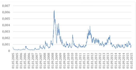
Since Table 3 does not allow to assess the evolution of the conditional variance over time, Figure 1 depicts its development from 1st May 2005 to 1st May 2015. For clarity reasons, the average of the conditional variance of all institutions in the system is taken. The graph shows a tranquil period in the beginning followed by a period of very high volatility from mid-2008 to mid-2009, represented by the high peaks during this time. The volatility decreases again thereafter but exhibits three more peaks: one in 2010, one in late-2011, and one in mid-2013. While the first and largest peaks can be explained by the global financial crisis, the three peaks thereafter represent the distressing events caused by the European debt crisis. Since the global financial crisis and the European debt crisis have been major system-wide shocks, it can be expected that these events also affected the ΔCoVaR measure.

Figure 1 Average conditional variance of all sample institutions (01.05.2005 – 01.05.2015)

0 0,001 0,002 0,003 0,004 0,005 0,006 0,007 01 .0 5. 20 05 01 .0 9. 20 05 01 .0 1. 20 06 01 .0 5. 20 06 01 .0 9. 20 06 01 .0 1. 20 07 01 .0 5. 20 07 01 .0 9. 20 07 01 .0 1. 20 08 01 .0 5. 20 08 01 .0 9. 20 08 01 .0 1. 20 09 01 .0 5. 20 09 01 .0 9. 20 09 01 .0 1. 20 10 01 .0 5. 20 10 01 .0 9. 20 10 01 .0 1. 20 11 01 .0 5. 20 11 01 .0 9. 20 11 01 .0 1. 20 12 01 .0 5. 20 12 01 .0 9. 20 12 01 .0 1. 20 13 01 .0 5. 20 13 01 .0 9. 20 13 01 .0 1. 20 14 01 .0 5. 20 14 01 .0 9. 20 14 01 .0 1. 20 15 01 .0 5. 20 15

(31)

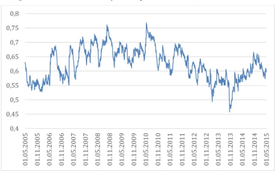
23 Figure 2 depicts the evolution of the dynamic conditional correlations from 1st May 2005 to 1st May 2015. Again, for clarity reasons the average of the dynamic conditional correlations of all banks in the system is taken. While the average dynamic conditional correlation is also influenced by the events of the global financial crisis and the European debt crisis, the impact is less pronounced than for the average conditional variance. Interestingly, while the average conditional variance exhibits peaks over the course of the year 2013, caused by the events of the European debt crisis, the average dynamic conditional correlations in contrast show decreasing correlations between the financial institutions and the system. This is somewhat surprising, as the correlations between a financial institution and the system are expected to increase in times of a crisis (Ang & Chen, 2002).

Figure 2 Average conditional correlation of all sample institutions (01.05.2005 – 01.05.2015)

5.2.3

Individual VaR

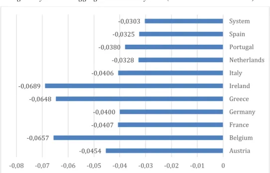
Using the estimation outputs that have been described above, daily 5% VaR-levels for each institution and the system itself have been calculated. Figure 3 depicts the average daily 5% VaR for each country. The figure shows that on average, Irish, Belgian, and Greek banks exhibited the highest individual VaR, whereas financial institutions from Spain, the Netherlands, and Portugal showed the lowest average VaR. Furthermore, Figure 3 shows that the unconditional VaR of the financial system is lower than the average VaR of each country. This can be explained by the diversification effect of the system, which consists of all sample institutions. The strong link between individual VaR and individual volatility becomes clear when comparing Table 2 to Figure 3, as the countries with the highest (lowest) average conditional variance are among the countries with the highest (lowest) average individual VaR-levels. 0,4 0,45 0,5 0,55 0,6 0,65 0,7 0,75 0,8 01 .0 5. 20 05 01 .1 1. 20 05 01 .0 5. 20 06 01 .1 1. 20 06 01 .0 5. 20 07 01 .1 1. 20 07 01 .0 5. 20 08 01 .1 1. 20 08 01 .0 5. 20 09 01 .1 1. 20 09 01 .0 5. 20 10 01 .1 1. 20 10 01 .0 5. 20 11 01 .1 1. 20 11 01 .0 5. 20 12 01 .1 1. 20 12 01 .0 5. 20 13 01 .1 1. 20 13 01 .0 5. 20 14 01 .1 1. 20 14 01 .0 5. 20 15

(32)

Figure 3 Average daily 5% VaR aggregated at country level (01.05.2005 – 01.05.2015)

To analyze the time-series behavior of the VaR, the evolution of the average 5% daily VaR of all sample institutions is depicted in Figure 4. Similarly to Figure 1, the average VaR first exhibits relatively low levels until mid-2008, where it begins to increase dramatically. This period of very high VaR-levels lasts until mid-2009 and can be explained by the global financial crisis. The average VaR decreases to lower levels thereafter, but like the average conditional variance shows three more peaks in mid-2010, in late-2011, and in mid-2013. These three peaks can be explained by the on-going European debt crisis. The resemblance of Figure 1 and Figure 4 is another indicator for the strong relation between individual volatility and individual VaR.

Figure 4 Average 5% daily VaR of all sample institutions (01.05.2005 – 01.05.2015)

-0,0454 -0,0657 -0,0407 -0,0400 -0,0648 -0,0689 -0,0406 -0,0328 -0,0380 -0,0325 -0,0303 -0,08 -0,07 -0,06 -0,05 -0,04 -0,03 -0,02 -0,01 0 Austria Belgium France Germany Greece Ireland Italy Netherlands Portugal Spain System 0 0,02 0,04 0,06 0,08 0,1 0,12 0,14 01 .0 5. 20 05 01 .1 1. 20 05 01 .0 5. 20 06 01 .1 1. 20 06 01 .0 5. 20 07 01 .1 1. 20 07 01 .0 5. 20 08 01 .1 1. 20 08 01 .0 5. 20 09 01 .1 1. 20 09 01 .0 5. 20 10 01 .1 1. 20 10 01 .0 5. 20 11 01 .1 1. 20 11 01 .0 5. 20 12 01 .1 1. 20 12 01 .0 5. 20 13 01 .1 1. 20 13 01 .0 5. 20 14 01 .1 1. 20 14 01 .0 5. 20 15

(33)

25

5.3

CoVaR and ∆CoVaR

5.3.1

CoVaR

After analyzing the estimation outputs and the idiosyncratic VaR of the financial institutions, the focus is now put on the empirical results regarding CoVaR and ∆CoVaR. Figure 5 below depicts the average daily 5% VaR and CoVaR by country. Recall, that the CoVaR is the VaR of the financial system conditional on an institution being in financial distress, i.e. its returns being at their VaR level.

Figure 5 shows that Spanish, French, and Portuguese banks cause the highest average CoVaR levels of the system when being in financial distress, and that financial institutions from Greece, Ireland, and the Netherlands cause the lowest average CoVaR levels of the system when being in financial distress. A possible explanation of this observation is that the Greek, Irish, and Dutch banks are less correlated with the system than financial institutions from Spain, France, and Portugal. Table 3 partly supports this explanation, since the banks from Greece, Ireland and the Netherlands are among the banks which exhibit the lowest average dynamic conditional correlation with the system, and Spanish and French banks are among the banks which exhibit the highest average dynamic conditional correlation with the system. However, while Portuguese financial institutions cause high average CoVaR levels for the system, their average dynamic conditional correlation with the system are among the lowest. Thus, systemic risk seems to be determined by more factors than just correlation with the system. Figure 5 also shows that all countries’ average CoVaR is larger than their average VaR. Furthermore, the relation between VaR and CoVaR appears to be rather weak, as low VaR-levels are paired with both high and low CoVaR-levels. Lastly, the average unconditional VaR of the system is, unsurprisingly, smaller than all average VaR’s of the system conditional on an individual institution being in distress, as denoted by CoVaR.

Figure 5 Average daily 5% VaR and CoVaR by country (01.05.2005 – 01.05.2015)

-0,09 -0,08 -0,07 -0,06 -0,05 -0,04 -0,03 -0,02 -0,01 0 Austria Belgium France Germany Greece Ireland Italy Netherlands Portugal Spain System

(34)

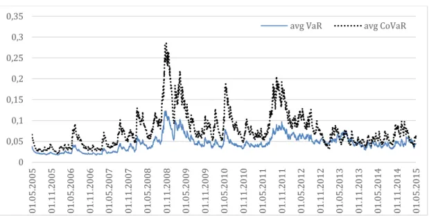
In order to compare the evolution of VaR and CoVaR over time, the average of the respective measure of all sample institutions is depicted in Figure 6. While Figure 5 indicates that there is a loose cross-sectional relation between VaR and CoVaR, Figure 6 suggests a close link between VaR and CoVaR in the time-series dimension. It is interesting to note that for almost every point in time, the average systemic risk caused by the financial institutions is larger than their average idiosyncratic r