Abstract—Energy production optimization has been traditionally
very important for utilities in order to improve resource consumption. However, load forecasting is a challenging task, as there are a large number of relevant variables that must be considered, and several strategies have been used to deal with this complex problem. This is especially true also in microgrids where many elements have to adjust their performance depending on the future generation and consumption conditions. The goal of this paper is to present a solution for short-term load forecasting in microgrids, based on three machine learning experiments developed in R and web services built and deployed with different components of Cortana Intelligence Suite: Azure Machine Learning, a fully managed cloud service that enables to easily build, deploy, and share predictive analytics solutions; SQL database, a Microsoft database service for app developers; and PowerBI, a suite of business analytics tools to analyze data and share insights. Our results show that Boosted Decision Tree and Fast Forest Quantile regression methods can be very useful to predict hourly short-term consumption in microgrids; moreover, we found that for these types of forecasting models, weather data (temperature, wind, humidity and dew point) can play a crucial role in improving the accuracy of the forecasting solution. Data cleaning and feature engineering methods performed in R and different types of machine learning algorithms (Boosted Decision Tree, Fast Forest Quantile and ARIMA) will be presented, and results and performance metrics discussed.
Keywords—Time-series, features engineering methods for
forecasting, energy demand forecasting, Azure machine learning. I. INTRODUCTION &BUSINESS DOMAIN
NERGY load forecasting has been traditionally a critical use case for utilities around the world. However, to meet the required accuracy, it has been a challenging task [1]. Since there are relatively large numbers of relevant variables that must be considered, several strategies have been attempted to deal with this complex problem. This is especially the case in microgrids [2] where many elements must work in tandem and optimized to meet the future demand of energy while avoiding waste of energy [3].
The load forecast solution for a microgrid setup is well demonstrated in recent use case we have worked on. A microgrid is a self-sufficient energy structure capable of balancing captive supply and demand resources to endure a constant service within a definite boundary [4]. From a technology point of view, a microgrid is an interconnected system of distributed, clean-power units, functioning independently or in collaboration with a larger electrical grid
F. Lazzeri is a Data Scientist II and I. Reiter is a Principal Data Science Manager at Microsoft - Algorithms and Data Science Department, Cambridge, MA 02142 USA (phone: (857) 453-6000; e-mail: [email protected], [email protected]).
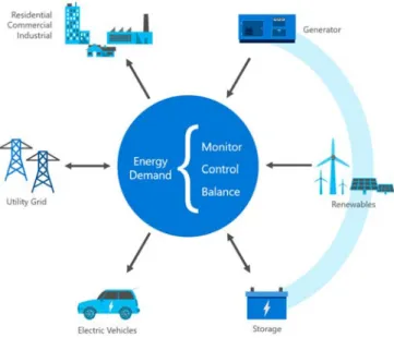
to produce high-quality power [5] (Fig. 1).
Fig. 1 Microgrid System
Microsoft has used Cortana Analytics Suite as a platform to build a cloud based solution for microgrid energy demand forecasting. It would generate short term load forecasts that allow the optimization of the electricity, steam and chilled water consumption.
II. DATA SOURCES AND DATA DESCRIPTION
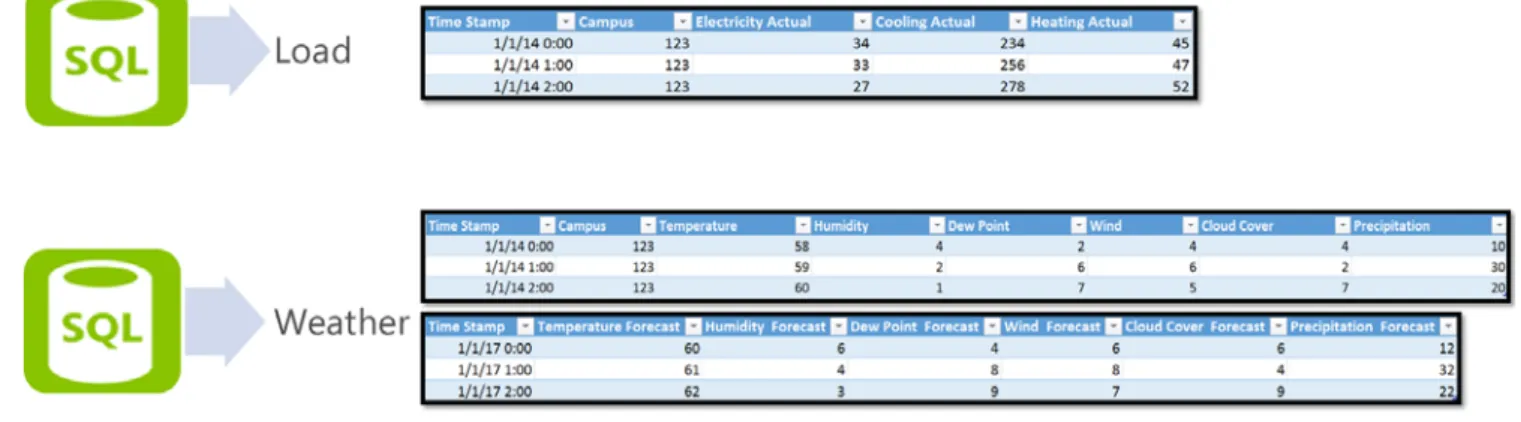
The raw data are generated from 30 meters (18 power meters, 6 steam meters and 6 chilled water meters). From the meters, data are aggregated and ingested into an on-prem SQL database. The data include hourly aggregated actual electricity consumption (in Kilowatt hour), chilled water consumption (in Tons per hour), and heating steam (in Pound per hour).
To improve the demand forecast accuracy, we also rely on external data sources. Historical data show strong correlation between outside weather data (such as temperature) and power consumption. For this reason, historical weather data is critical to build energy load forecasting models. For this solution, we used weather data obtained from a 3rd party provider. It includes hourly temperature, humidity, dew point, wind, cloud cover, precipitation data (Fig. 2).
III. APPROACH
In data science terms, the microgrid load forecasting can be categorized a time series problem. A typical approach is making use of historical demand data that is time stamped. To
F. Lazzeri, I. Reiter
Load Forecasting in Microgrid Systems with R and
Cortana Intelligence Suite
E
accomplish higher level of forecasting accuracy, we also used
external factors that may add more predictability. In the case of energy demand this relates mostly to weather data.
Fig. 2 Load and Weather Data IV. DATA PROCESSING AND FEATURE ENGINEERING
The first step to be taken is to process the available data and extract goo predictors from it. In time series, the feature extraction goal is to identify time related trends, seasonality, auto-correlation (correlation over time), and transform those into a model.
Neutrally, the available raw data may include missing values and outliers. To deal with that, we have developed Azure ML service which deploys R based algorithms that allow us to compare trends across weeks and adjust values so to obtain greater trend similarity. R was also the main tool that we have used for the feature extraction part (Fig. 3).
Fig. 3 Data Cleaning and Feature Engineering with Execute R Script Few of the features we have used include:
Time driven features: These features are created from the timestamp data and column, and they are transformed into categorical features like:
Hour of day, which refers to the hour of the day and has values from 0 to 23.
Day of week, which refers to the week day and has values from 1 (Sunday) to 7 (Saturday).
Month of year, that denotes the month of a year and creates values from 1 (January) to 12 (December).
Weekend, that represents a binary value feature and has values of 0 for weekdays or 1 for weekend [6].
BusinessTime - This is a binary value feature that takes the values of 0 for time window between 5PM until 8AM or 1 for time window from 8AM until 5PM.
Ismorning - This is a binary value feature that takes the values of 0 for time that is not morning or 1 for morning.
Fourier terms: These features represent weights that are created from time data and are used to measure the seasonality in the data. Since our data may have multiple seasons, it is often recommended to build multiple Fourier terms. Moreover, demand values may show yearly, weekly, and daily seasons/cycles, which result in three different Fourier terms [7].
Independent measurement features: These variables embrace all the data points that we need to use as predictors in our model. For this purpose, we exclude the dependent feature that needs to be predicted [8].
Lag features: These are time-shifted values of the actual demand data. In this context, feature lag1 will hold the demand value in the previous hour relative to the current timestamp [9].
For the Electricity consumption forecast we built the following lag features: Lag72, Lag73, Lag74, Lag75, Lag76, Lag144, Lag216.
For the Chilled Water consumption forecast we built the following lag features: Lag 72, 73, Lag74, Lag75, Lag76, Lag96, Lag120, Lag144, Lag168, Lag192.
For the Steam consumption forecast we built the following lag features: Lag 72, Lag73, Lag74, Lag75, Lag76, Lag216, Lag240, Lag264, Lag288, Lag312.
V. MODELING
There are three forecasting models implemented utilizing Azure Machine Learning for electricity, chilled water and steam respectively. For electricity and steam forecasting models, we have used a Boosted Decision Tree regression. For the chilled water forecasting models, we have found that Fast Forest Quantile regression to work the best.
VI. EVALUATION
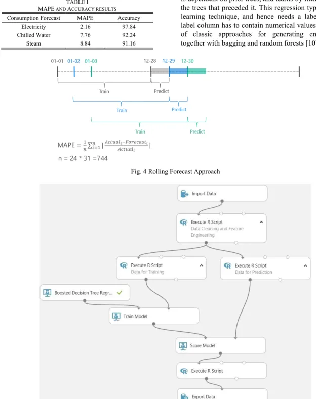
To evaluate our model performance, we use the Mean Absolute Percent Error (MAPE) metric, that is a measure of prediction accuracy of a forecasting method in statistics: the difference between actual value and forecast value is divided by the actual value again to produce percentage metric.
The actual performance evaluation is done through rolling window forecast (Fig. 4).
Table I summarizes MAPE and accuracy of some of our forecasted results (testing period - January 2013 to November 2015; scoring period - December 2015).
TABLEI
MAPE AND ACCURACY RESULTS
Consumption Forecast MAPE Accuracy Electricity 2.16 97.84 Chilled Water 7.76 92.24 Steam 8.84 91.16
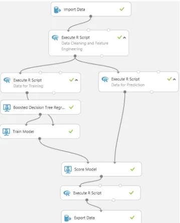
VII. MACHINE LEARNING EXPERIMENTS IN AZUREML We built 3 different forecasting models in AzureML. For electricity and chilled water, we used a Boosted Decision Tree Regression (Figs. 5, 6). This regression creates an ensemble of regression trees using boosting. Boosting means that each tree is dependent on prior trees, and learns by fitting the residual of the trees that preceded it. This regression type is a supervised learning technique, and hence needs a labeled dataset. The label column has to contain numerical values. Boosting is one of classic approaches for generating ensemble models, together with bagging and random forests [10].
Fig. 4 Rolling Forecast Approach
Fig. 5 Boosted Tree Regression Experiment for Electricity Forecast
Fig. 6 Boosted Tree Regression Experiment for Steam Forecast
For the Chilled Water forecast, we used a Fast Forest Quantile Regression with Tune Model Hyperparameters (Fig. 7).
Fast Forest Quantile Regression generates a regression model that can predict values for multiple numbers of quantiles. Quantile regression forest provides a non-parametric method for predicting conditional quantiles for high-dimensional predictor features [11]. We also performed other analyses using different machine learning algorithms; however, we obtained the best accuracy by using Boosted Decision Tree and Fast Forest Quantile regressions. We tried the two following approaches:
ETS (Exponential Smoothing) - ETS is a group of methods that utilize weighted average of recent data elements to estimate the next data element. The main goal is to assign higher weights to more recent data points and progressively reduce this weight for older values [12].
ARIMA (Auto Regression Integrated Moving Average) - Auto-regression methods take previous time series’ values to estimate next data element. This type of methods uses also differencing techniques that include calculating the difference between data elements and including those instead of the original measured value. Finally, this type of methods uses the moving average techniques. Using all these methods in various ways and in parallel is what creates the family of ARIMA methods [13].
Fig. 7 Fast Forest Quantile Regression for Chilled Water Forecast
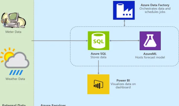
VIII. SOLUTION ARCHITECTURE
Cortana Analytics Suite is the foundation for deploying this solution. We have used SQL Azure and Azure Machine Learning as well as Azure Data Factory (ADF) to orchestrate
data movement and invoke the Azure Machine Learning web services at a predetermined schedule. PowerBI dashboard is used for the visualization of historical data and forecast results. Fig. 8 shows the solution architecture.
Fig. 8 Solution Architecture IX. CONCLUSION
By making use of Cortana Intelligence-based framework, we have managed to build and deploy a solution that predicts hourly load forecast results for a microgrid system.
In a microgrid situation as in this case, there could be multiple energy resources that need to be optimized [14], [15]. We found that each one of them may have posed different patterns and therefore tuning the performance must be done on each resource individually. We have also found that for those types of forecasting models, weather data (temperature, wind, humidity and dew point etc. etc.) can play a different role in improving the accuracy of your model.
Additionally, we realized that deploying and operationalizing a machine learning based forecasting solution requires a reliable platform. Many companies are making their journey of implementing the full-scale automation that is needed to harness the full benefit of the cloud. Taking advantage of Cortana Analytics Suite allows microgrids to not only improve the model performance over time (via model retraining) but also to enables fast and reliable deployment framework for such use cases. This ensures drive a long term and continues business value generation from machine learning and predictive analytics technologies.
Next step will be to build a scalable energy load forecasting solution, to scale out across multiple microgrid sites and allow any utility to easily adopt and operationalize the solution for their microgrid systems. This solution can be accomplished also thanks to R, the most used languages in the data science
and machine learning community: with R we can perform scalable data analytics, select the appropriate compute infrastructure, use distributed algorithms and out-of-memory computational techniques.
REFERENCES
[1] W. Su, J. Wang, “Energy Management Systems in Microgrid Operations”, The Electricity Journal, vol. 25, no. 8, pp. 45–60, October 2012.
[2] M.A Ancona, L. Branchini, A. De Pascale, F. Melino, “Smart District Heating: Distributed Generation Systems’ Effects on the Network”,
Energy Procedia, vol. 75, pp. 1208-1213, 2015.
[3] T.S. Ustun, C. Ozansoy, A. Zayegh, “Recent developments in microgrids and example cases around the world: A review”, Renewable
and Sustainable Energy Reviews, vol. 15, no. 8, pp. 4030-4041, October
2011.
[4] https://doh.dc.gov/sites/default/files/dc/sites/ddoe/service_content/attach ments/DOEE%20Microgrid%20101%20Presentation%20%28Sept%202 015%29.pdf, September 2015.
[5] http://www.nrg.com/renewables/technologies /microgrids/, August 2016. [6]
https://github.com/edsfocci/azure-content/blob/master/articles/cortana-analytics-playbook-demand-forecasting-energy.md, January 2016. [7] http://www.reed.edu/physics/courses/Physics331.f08/pdf/Fourier.pdf,
2008.
[8] M. Prabhugoud, K. Peters, J. Pearson, M. A. Zikry, “Independent measurement of strain and sensor failure features in Bragg grating sensors through multiple mode coupling”, Sensors and Actuators A Physical, vol. 135, no. 2, pp. 433-442, April 2007.
[9] https://gallery.cortanaintelligence.com/CustomModule/Generate-Lag-Features-1, October 2016.
[10] https://msdn.microsoft.com/en-us/library/azure/dn905801.aspx, June 9, 2016.
[11] N. Meinshausen, “Quantile Regression Forests”, Journal of Machine
Learning Research, vol. 7, pp. 983-999, 2006.
[12] http://stat.cmu.edu/~hseltman/618/LNTS4.pdf, March 3, 2016.
[13] X. Chang, M. Gao, Y. Wang, X. Hou, “Seasonal autoregressive integrated moving average model for precipitation time series”, Journal of Mathematics and Statistics, vol. 8, no. 4, pp. 500-505, 2012.
[14] K. Xian-guo, L. Zong-qi, Z. Jian-hua, “New Power Management Strategies for a Microgrid with Energy Storage Systems”, Energy Procedia, vol. 16, part C, pp. 1678-1684, 2012.
[15] H. Jiayi, J. Chuanwen, X. Rong, “A review on distributed energy resources and MicroGrid”, Renewable and Sustainable Energy Reviews,
vol. 12, no. 9, pp. 2472-2483, December 2008.