Wright State University Wright State University
CORE Scholar
CORE Scholar
Browse all Theses and Dissertations Theses and Dissertations
2018
Multiple Drone Detection and Acoustic Scene Classification with
Multiple Drone Detection and Acoustic Scene Classification with
Deep Learning
Deep Learning
Hari Charan VemulaWright State University
Follow this and additional works at: https://corescholar.libraries.wright.edu/etd_all
Part of the Computer Engineering Commons, and the Computer Sciences Commons
Repository Citation Repository Citation
Vemula, Hari Charan, "Multiple Drone Detection and Acoustic Scene Classification with Deep Learning" (2018). Browse all Theses and Dissertations. 2221.
https://corescholar.libraries.wright.edu/etd_all/2221
This Thesis is brought to you for free and open access by the Theses and Dissertations at CORE Scholar. It has been accepted for inclusion in Browse all Theses and Dissertations by an authorized administrator of CORE Scholar. For more information, please contact [email protected].
Multiple
Drone
Detection
and
Acoustic
Scene
Classification
with
Deep
Learning
A
Thesis
submitted
in
partial
fulfillment
of
the
requirements
for
the
degree
of
Master
of
Science
by
Hari
Charan
Vemula
B.Tech,
GITAM
University,
2015
2018
WRIGHT STATE UNIVERSITY GRADUATE SCHOOL
12/14/2018 I HEREBY RECOMMEND THAT THE THESIS PREPARED UNDER MY SUPERVISION BY Hari Charan Vemula ENTITLED Multiple Drone Detection and Acoustic Scene
Classification with Deep Learning BE ACCEPTED IN PARTIAL FULFILLMENT OF THE REQUIREMENTS FOR THE DEGREE OF Master of Science.
_____________________________ John C. Gallagher, Ph.D.
Thesis Director
_____________________________ Mateen M. Rizki, Ph.D.
Chair, Computer Science and Engineering
Committee on Final Examination: ________________________________ John C. Gallagher, Ph.D. ________________________________ Mateen M. Rizki, Ph.D. ________________________________ Thomas Wischgoll, Ph.D. ________________________________ Barry Milligan, Ph.D.
ABSTRACT
Vemula, Hari Charan. M.S., Department of computer science and Engineering, Wright State Uni-versity, 2018.Multiple Drone Detection and Acoustic Scene Classification with Deep Learning.
Classification of environmental scenes and detection of events in one’s environment from audio signals enables one to create better-planning agents, intelligent navigation sys-tems, pattern recognition syssys-tems, and audio surveillance systems. This thesis will ex-plore the use of Convolutional Neural Networks(CNN’S) with spectrograms and raw audio waveforms as inputs to Deep Neural Networks with hand engineered features extracted from large-scale feature extraction schemes to identify the acoustic scenes and events. The first part focuses on building an audio pattern recognition system capable of detecting the if there are zero, one, or two DJI phantoms in the scene within the range of a stereo mi-crophone. The ability to distinguish the presence multiple UAV’s could be used to aug-ment information from other sensors less capable of making such determinations. The second part of the thesis focuses on building an acoustic scene detector to Task 1a in the DCASE2018 challenge(http://dcase.community/challenge2018/index). In both cases, this document will explain the pre-processing techniques, CNN and DNN architectures used, data augmentation methods including the use of Generative Adversarial Networks(GAN’s), and performance results compared to existing benchmarks when available. This thesis will conclude with a discussion of how one might expand the techniques in the construction of commercial off the shelf audio scene classifier for multiple UAV detections.
Contents
1 Introduction 1
1.1 Drone Detection with audio. . . 1
1.1.1 Problem Statement . . . 1
1.1.2 Related Work . . . 2
1.1.3 Aim and Scope . . . 3
1.2 Detection and Classification of Environmental Sound Events . . . 4
1.2.1 Problem Statement . . . 4
1.2.2 Related Work . . . 5
1.2.3 Aim and Scope . . . 5
1.3 Document Overview . . . 6
2 Background 7 2.1 Dataset Design . . . 8
2.1.1 Drone Detection Dataset . . . 8
2.1.2 DCASE Dataset . . . 10
2.2 Mathematical View of Signal Processing . . . 14
2.2.1 Nyquist-Shannon Sampling Theorem . . . 14
2.2.2 Convolution Theorem . . . 14
2.2.3 Discrete Fourier Transform. . . 15
2.2.4 Short Time Fourier Transform . . . 16
2.2.5 Mel-Scale . . . 17
2.2.6 Log-MelSpectrogram . . . 18
2.2.7 Discrete Cosine Transform . . . 19
2.2.8 Harmonic Percussive Source Separation . . . 19
2.3 Comparison between variants of Spectrograms. . . 21
2.4 Convolutional neural networks . . . 23
2.4.1 Convolutional layer. . . 24 2.4.2 Activation Layer . . . 26 2.4.3 Pooling Layer. . . 26 2.4.4 Dense Layers . . . 28 2.5 Hyper Parameters . . . 28 2.5.1 Gradient Descent:. . . 28
2.5.2 Optimizing Gradient Descent . . . 30
2.5.3 Regularization techniques . . . 33
2.5.4 Initializtion and Transformation Hyper-Parameters . . . 33
2.6 Principal Component Analysis . . . 35
2.7 Random Forest Algorithm . . . 37
2.8 Libraries . . . 38 2.8.1 Kapre . . . 38 2.8.2 librosa. . . 38 39 2.8.3 openSMILE. . . . 3 PerformanceMeasures 43 3.1 Confusion Matrix . . . 44
3.2 Micro, Macro and Weighted Averages . . . 45
3.3 Receiver Operating Characteristic curve(ROC) . . . 47
3.4 Precision-Recall Curves. . . 50
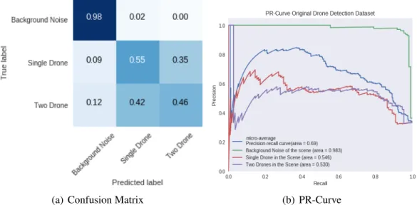
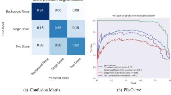
4 Experiments: Drone Detection 51 4.1 Multiple Drone Detection . . . 51
4.2 Experiment 1: PCA and TSNE visualization . . . 52
4.3 Experiment 2: Random Forest Algorithm with SMILE988 Features . . . . 54
4.4 Experiment 3: DNN with SMILE988 Features . . . 56
4.5 Experiment 4: DNN with SMILE200 features . . . 58
4.6 Experiment 5: CNN with Spectrograms . . . 59
4.6.1 CNN with Raw Spectrograms . . . 61
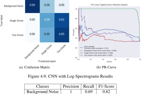
4.6.2 CNN with Log-Spectrograms . . . 61
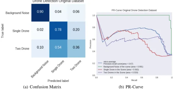
4.6.3 CNN with Mel-Spectrograms with 128 Mels . . . 63
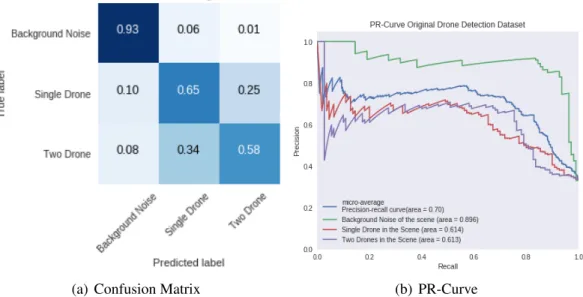
4.6.4 CNN with Log-Mel Spectrograms with 40 Mels. . . 64
4.6.5 CNN with Log-Melspectrograms with 60 mel filters . . . 66
4.6.6 CNN with Log-Mel Spectrograms with 80 Mels. . . 66
4.6.7 CNN with Log-Mel Spectrograms with 128 Mels . . . 67
4.6.8 CNN with Log-Mel Spectrograms with 200 Mels . . . 69
4.7 Experiment 6: CNN with Harmonic Percussive Source Separation . . . 70
4.8 Experiment 7: CNN with Raw Audio Forms . . . 71
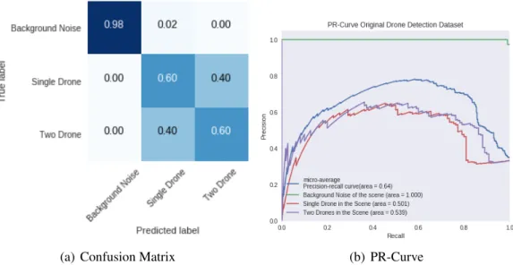
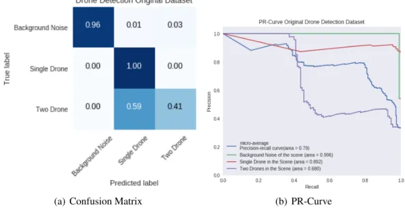
4.9 Drone Detection Dataset with Generative Models . . . 72
5 Augmenting Drone Detection Dataset 74 6 Experiments: Drone Detection with Augmented Dataset 75 6.1 Experiment1: PCA and TSNE analysis . . . 75
6.2 Experiment 2: Random Forest Algorithm with SMILE 988 features . . . . 78
6.3 Experiment 3: SMILE988 with DNN. . . 80
6.4 Experiment 4: DNN with SMILE200 features . . . 81
6.5 Experiment 5: CNN with Spectrograms . . . 82
6.5.3 CNN with Log-Mel Spectrograms with 40 Mels. . . 84
6.5.4 CNN with Log-Mel Spectrograms with 60 Mels. . . 84
6.5.5 CNN with Log-Mel Spectrograms with 80 Mels. . . 85
6.5.6 CNN with Log-Mel Spectrograms with 128 Mels . . . 86
6.5.7 CNN with Log-Mel Spectrograms with 200 Mels . . . 87
6.6 Experiment 6: Harmonic Percussive Source Separation . . . 91
7 Experiments: DCASE 92 7.1 Baseline System . . . 92
7.1.1 Baseline System . . . 92
7.2 PCA and TSNE visualization for DCASE SMILE988 Features . . . 94
7.3 Random Forest Algorithm on DCASE SMILE988 Features . . . 95
7.4 PCA and TSNE visualization for DCASE SMILE6k Features . . . 98
7.5 Random Forest algorithm for DCASE SMILE6K features . . . 100
7.6 DNN with SMILE988 features . . . 103
7.7 DNN with SMILE6K features . . . 106
7.8 CNN: Extended Baseline Model with data augmentation . . . 107
7.8.1 CNN with RawAudio waveforms . . . 107
7.8.2 Sub-class Indoor Classification. . . 111
7.8.3 Sub-class Outdoor Classification . . . 111
7.8.4 Sub-class vehicle Classification . . . 115
8 Results, Discussion and Future Work 117 8.1 Results. . . 117
8.1.1 Multiple Drone Detection . . . 117
8.1.2 DCASE . . . 118
8.2 Discussion. . . 120
8.2.1 Multiple Drone Detection . . . 120
8.2.2 DCASE . . . 121
8.2.3 Hyper-Parameter Search Space and statistical significance of results 122 8.3 Conclusions . . . 123
8.3.1 Multiple Drone Detection . . . 123
8.3.2 DCASE . . . 124
8.3.3 Future Work . . . 125
List of Figures
2.1 Pipeline Diagram for Design of Drone Detection system . . . 7
2.2 Hardware used in Recording Drone audio . . . 9
2.3 Sample spectrograms Drones audio. . . 9
2.4 Signal Amplification . . . 11
2.5 Sample Spectrograms for DCASE classes . . . 13
2.6 Discre Fourier Transform. . . 15
2.7 Window functions . . . 16
2.8 Mel scale vs Hertz scale. . . 17
2.9 Mel Filter Bank with 40 mel filters . . . 18
2.10 Harmonic Percussive Source Separation . . . 20
2.11 Visual features of sound in spectro-temporal domain. . . 22
2.12 Two channel Convolutional Neural Network Architecture for audio classi-fication . . . 24
2.13 Convolution operation in CNN . . . 26
2.14 Max and Average Pooling. . . 27
2.15 Convex Error Surface . . . 31
2.16 Equations for Batch-Normalization . . . 34
2.17 Activation Functions. . . 35
3.1 Sample Confusion Matrix for multi-class classification . . . 44
3.2 PR and ROC plots . . . 49
4.1 SMILE988 Data Visualization for Drone Detection dataset . . . 53
4.2 40 Most Contributing features for the Random Forest algorithm . . . 55
4.3 Confusion Matrix for Random Forest algorithm . . . 56
4.4 DNN with smile988 . . . 57
4.5 DNN with SMILE988 Results . . . 58
4.6 DNN with SMILE200 Results . . . 59
4.7 CNN with Spectrograms . . . 60
4.8 CNN with raw Spectrograms Results . . . 62
4.12 CNN with Log-Mel Spectrograms with 60 Mels Results. . . 66
4.13 CNN with Log-Mel Spectrograms with 80 Mels Results . . . 67
4.14 CNN with Log-Mel Spectrograms with 128 Mels Results . . . 68
4.15 CNN with Log-Mel Spectrograms with 200 Mels Results . . . 69
4.16 CNN with Harmonic-Percussive Source Separation Results . . . 70
4.17 CNN with 3-channel Raw audio waveforms Results . . . 72
4.18 WaveGan for Drone Audio Generation . . . 73
6.1 SMILE988 data visualization for augmented Drone detection dataset . . . . 77
6.2 Confusion Matrix for Random Forest algorithm . . . 78
6.3 40 Most Contributing features for the Random Forest algorithm . . . 79
6.4 DNN with SMILE988 Results . . . 80
6.5 DNN with SMILE200 Results . . . 81
6.6 CNN with raw Spectrograms Results . . . 83
6.7 CNN with Log-Spectrograms Results . . . 84
6.8 CNN with Melspectrograms with 128 Mel filters Results . . . 85
6.9 CNN with Log-MelSpectrograms with 40 Mels Results . . . 86
6.10 CNN with Log-MelSpectrograms with 60 Mels Results . . . 87
6.11 CNN with Log-MelSpectrograms with 80 Mels Results . . . 88
6.12 CNN with Log-MelSpectrograms with 128 Mels Results . . . 89
6.13 CNN with Log-MelSpectrograms with 200 Mels Results . . . 90
6.14 CNN with Harmonic Percussive Source Separation Results . . . 91
7.1 Baseline System Architectue . . . 93
7.2 Data Visualization in reduced dimensions for DCASE SMILE 988 . . . 94
7.3 30 Most Contributing features for the Random Forest algorithm . . . 96
7.4 Confusion Matrix for the Random Forest algorithm . . . 97
7.5 Data Visualization in reduced dimensions for SMILE6k . . . 98
7.6 40 Most Contributing features for the Random Forest algorithm . . . 101
7.7 Confusion Matrix for the Random Forest algorithm . . . 102
7.8 DNN architecture with SMILE features . . . 104
7.9 DNN with DCASE SMILE988 features on DCASE . . . 105
7.10 DNN with DCASE SMILE6k features on DCASE . . . 106
7.11 Short Figure Caption . . . 108
7.12 CNN with DCASE Extended baseline model and data augmentation . . . . 109
7.13 CNN with raw audio waveforms . . . 110
7.14 Hierarchical CNN for Acoustic Scene Classification . . . 112
7.15 CNN for Hierarchical class classification . . . 113
7.16 CNN for Hierarchical class classification Sub-class Indoor . . . 114
7.17 CNN for Hierarchical class classification sub-class Outdoor. . . 115
7.18 CNN for Hierarchical class classification sub-class Vehicle . . . 116
8.1 Multiple Drone Detection Results . . . 119
List of Tables
2.1 Anatomy of Drone detection dataset . . . 10
2.2 Anatomy of the DCASE dataset . . . 12
2.3 openSMILE’s low-level descriptors . . . 41
2.4 Functionals(Statistical, polynomial regression, and transformations) avail-able in openSMILE . . . 41
4.1 Most Contributing Features for First 3-Principal Components for Drone detection dataset. . . 54
4.2 Hyper Parameters . . . 57
4.3 Classification Report for DNN with SMILE988 Features . . . 58
4.4 Classification Report for DNN with SMILE200 Features . . . 59
4.5 Input Feature Vector for CNN with Spectrograms . . . 60
4.6 Hyper Parameters for CNN with Spectrograms . . . 61
4.7 Classification Report for CNN with Spectrograms . . . 62
4.8 Classification Report for CNN with Log-Spectrograms . . . 63
4.9 Classification Report for CNN with Mel-Spectrograms with 128 Mels . . . 64
4.10 Classification Report for CNN with Log-Mel Spectrograms with 40 Mels . 65 4.11 Classification Report for CNN with Log-Mel Spectrograms with 60 Mels . 66 4.12 Classification Report for CNN with Log-Mel Spectrograms with 80 Mels . 67 4.13 Classification Report for CNN with Log-Mel Spectrograms with 128 Mels . 68 4.14 Classification Report for CNN with Log-Mel Spectrograms with 200 Mels . 69 4.15 Classification Report for CNN with Harmonic-Percussive Source Separation 70 4.16 Classification Report for CNN with 3-channel Raw-audio Waveforms . . . 72
5.1 Anatomy of Augmented Drone Detection Dataset . . . 74
6.1 Most Contributing Features for First 3-Principal Components for Augmented Drone Dataset . . . 76
6.2 Classification Report for DNN with SMILE988 Features . . . 80
6.3 Classification Report for DNN with SMILE200 Features . . . 81
6.4 Classification Report for CNN with raw Spectrograms . . . 83
6.7 Classification Report for CNN with Log-Mel Spectrograms with 40 Mels . 86 6.8 Classification Report for CNN with Log-Mel Spectrograms with 60 Mels . 87 6.9 Classification Report for CNN with Log-Mel Spectrograms with 80 Mels . 88 6.10 Classification Report for CNN with Log-Mel Spectrograms with 128 Mels . 89 6.11 Classification Report for CNN with Log-Mel Spectrograms with 200 Mels . 90 6.12 Classification Report for CNN with Harmonic Percussive Source Separation 91
7.1 Class-wise Performance of DCASE Baseline system . . . 93
7.2 Most Contributing Features for First 3-Principal Components for DCASE SMILE988 . . . 95
7.3 Most Contributing Features for First 3-Principal Components for DCASE SMILE6K . . . 99
7.4 Classification report DNN with DCASE SMILE988 features . . . 105
7.5 Classification report DNN with DCASE SMILE6k features . . . 106
7.6 Classification report for Extended baseline CNN with data augmentation . . 109
7.7 Classification report for CNN with raw waveforms . . . 110
7.8 Classification report for Hierarchical CNN . . . 113
7.9 Classification report for Hierarchical CNN sub-class Indoor . . . 114
7.10 Classification report for Hierarchical CNN sub-class Outdoor . . . 115
7.11 Classification report for Hierarchical CNN sub-class Vehicle . . . 116
Acknowledgment
I would like to take this opportunity to extend my thanks to my advisor Dr. John C.Gallagher for being patient, and guiding me all along the journey of my thesis. I would also, like to thank Google for making the GPU computing accessible to masses for free with Colabora-tory.
Dedicated to My Dad and Mom.
1 Introduction
This thesis work consists of two parts, The first part deals with the problem of multiple drone detection followed by the 2018 Kaggle challenge on Detection and Classification of Acoustic Scenes and Events(DCASE) dataset.
1.1
Drone Detection with audio
1.1.1
Problem Statement
Unmanned aircraft systems, in the last decade has witnessed a significant increase in its usage in commercial, recreational and military applications. The US Federal Aviation Administration[1] defines an unmanned aircraft as a device used for flight in the air with no on-board pilot and whose range in size is from wingspans of six inches to 246 feet, and can weight from approximately forty ounces to over 25,600 pounds. The functional categories of drones include Target and Decoy, Reconnaissance, Combat, Logistics, civil and commercial. The initial applications of unmanned aerial vehicles were limited to the domains of military applications. However, with the increase in the technology, the de-sign and development of the drones have got cheaper, and the domain of their usage has rapidly expanded. Currently, the drones are employed in disaster management[2], product delivery systems[3,4], search and rescue missions[5], herding a flock of birds approaching
the list is exponentially increasing.
Drones along with their numerous applications in the airspace come with security risks which include airspace threats, privacy, using the vehicle as a weapon, corporate espionage, vehicle collision, and drone-based hacking. There are two phases in designing and enforc-ing regulations for drone usage, the first phase deals with drone detection and is followed by how to respond in the event if a drone being detected. The scope of this thesis work only focuses on the first phase of drone detection. FAA has implemented ”no-drone-zone” over sensitive areas in the US, which never really worked preventing the drones in appearing in those areas, and a need for a technical solution for detecting drones has called for after the incident of a drone crashing near the white house[9]. One of the most prominent solutions is to force the drone manufacturing companies like DJI to embed a transponder system like GeoSpatial Environment Online lock[10] into the devices to geofence the devices from fly-ing into the ”no-drone-zones.” However, this is not a practical solution, due to the increase in the open technology over the World Wide Web, which enabled drone users to build drone right from scratch, and monitoring them would be a near to impossible task. The military may use very expensive RADAR systems to detect Drones, however, they are expensive, and their design of functionality is not suitable in the urban environment. There also ex-ists a few end-to-end commercial solutions employing wide variety of complex sensory systems like [11] using acoustic sensors, [12] employing radar, radio frequency, acoustic, camera and thermal sensors, [13] employing a radio frequency sensors for RF programmed drones, along with RADAR solid-state Doppler for non-RF programmed drones.
1.1.2
Related Work
As far as the author’s knowledge is concerned, there exists no research in classifying mul-tiple quadrotors in the scene. And, the only second one to employ convolutional neural networks for solving the problem of drone detection. However, few studies were found in
crossing rate, reflection coefficients, the slope of the spectrum, spectral centroid, spectral roll-off, MFCC’s and Mel-spectrograms are used in those studies. [14] in his/her work used Mel-spectrograms with convolutional neural networks, Gaussian Mixture Models and recurrent neural networks, with the reported detection accuracy of 64.15 with CNN and 80.09 with GMM. [16] employed hand engineered features like zero-crossing rate, linear predictive coding representing the spectral envelope of the audio signal, are used with the DSP processor creating the database of the features, during inference the values attained for the corresponding features are compared to the ones in the database in predicting the presence or absence of the drone. In the work of [15], support vector machines are em-ployed on features including short time energy, temporal roll-off, temporal centroid, zero crossing rate, spectral centroid, spectral roll-off, and Mel frequency cepstral coefficients.
1.1.3
Aim and Scope
Unlike naturally occurring sounds, Drones do have distinctive sound characteristics. Lever-aging on this, the first part of the thesis work focuses on building an off-the-shelf audio inference system for detection of the multiple drones in the scene. In work here we will use raw spectrograms, log-Melspectrograms, harmonic-percussive source separation and raw audio waveforms of the audio samples collected from stereo microphones (three spec-trograms per sample, one for each channel of the stereo input and one for the difference between the two channels) as an input to the CNN’s to determine the number of drones present in the area. The use of spectrograms and raw audio waveforms as inputs converts the detection problem into a vision problem. The natural positional scaling abilities of the CNN capturing spectro-temporal features should come into play.
This part of the thesis seeks to answer the following questions:
1) Is it possible to build an audio inference system for detecting the presence of multiple drones in the area with inexpensive Commercial Off the Shelf Equipment(COTS)?
drone detection for practical use?
3) Could the techniques used in the drone detection system prototype beat the commercial drone detection systems in performance?
The questions will be addressed in the context of a comprehensive comparison be-tween the performance of the DNN with large-scale feature extraction schemes, CNN with variants of spectrograms in both frequency scale and the psychoacoustic scales and the per-formance of the recent sample level CNN’s architectures for the detector working on raw audio forms in time-domain.
1.2
Detection and Classification of Environmental Sound
Events
1.2.1
Problem Statement
Classification of Environmental sound events is a subfield of computational auditory scene analysis which focuses on the creation of intelligent machine listening systems identifying acoustic scenes similar to human listeners. The applications include tagging millions of hours of audio on the web, increased precision in understanding the environment for au-tonomous systems, audio surveillance systems, noise mitigation and off-the-shelf pattern recognition systems. Since the year 2010, it has been observed how benchmark datasets like Imagenet paved the way for the field of computer vision to achieve above human-level performance on Image classification tasks. The DCASE data set is the Imagenet of Acous-tic scene and event classification. To further expand the intuition developed in part 1, this part of the thesis focuses on the classification of environmental sound events. A baseline system employing a two layer convolutional neural networks with a reported accuracy of
59 percent is provided by the challenge organizers.
1.2.2
Related Work
Since the inception of the DCASE challenge in the year 2013, over 50 submissions are made every year, However, until 2016 submissions were based on statistical and proba-bilistic models with hand engineered features[17, 18, 19, 20, 21, 22]. Since 2016, The convolutional neural networks have been employed in one form or the other in almost all the state of the art approaches[23,24,25,26,27,28].
1.2.3
Aim and Scope
Unlike, the sounds obtained in Automatic Speech Recognition (ASR) and environmental event detection the acoustic scene detection sounds are continuous. In the detection of an acoustic scene class, firstly, all the events happening in the scene are identified, and by learning the relationship between the detected events will help in predicting the acoustic scene class. It becomes harder in hand engineering the features which capture such complex relationships. In the scope of this thesis work, large-scale feature extraction schemes were employed followed by spectrograms and its variants including Mel Spectrograms in log scale.
The final objective is to attain far off better performance over the baseline system, Understanding the suitable CNN architectures in solving the problem.
This part of the thesis seeks to answer the following questions:
1) How would the performance of the deep learning models working on raw data in the spectro-temporal domain, compare to the performance of the statistical and probabilistic models working with Hand engineered features of both time and frequency domain?, What is the effect of the infinitely strong prior of CNN’s over its weights on the solution?
in the field of computer vision and deep learning. Which include the effect of Batch Normalization, Exponential Linear Units(ELU), Rectified Linear Unit (ReLU), addition of Gaussian Noise in training, and Cyclic Learning Rates(CLR).
3) Which of the CNN architectures yield better generalization performance and faster con-vergence with spectro-temporal data.
4) Which of the variants of spectrograms can yield better performance with Convolutional Neural Networks.
5) What is the performance of convolutional Neural Networks on raw audio waveforms in time-domain?
1.3
Document Overview
This document is organized as follows: This document is organized as follows: Chap-ter two will provide the background information on the techniques used for the Signal Processing, Feature Extraction and Classification algorithms employed in the scope of this thesis work along with the in brief discussion on the openSMILE large-scale feature extrac-tion library. Also, it discusses the data collecextrac-tion environment and the dataset organizaextrac-tion for the custom collected dataset for multiple drone detection. Chapter three discusses the performance metrics used in the scope of this thesis work. Chapter four and Chapter six deals with the experiments performed on the multiple drone detection dataset, and Chapter seven deals with experiments performed on the DCASE dataset. Chapter five explains the process involved in augmenting the drone detection dataset. Chapter eight discusses the results obtained for both datasets, along with the comparison between the performance of architectures and feature extraction schemes employed in the experiments. Followed by it discusses the comparison with the objective of this thesis with the results obtained and the significant observation that was made in the way through the completion of this thesis, and the future work and the possible extension that could be made to this work.
2 Background
This chapter provides the background information needed for the design and deployment of the multiple Drone detection system and the Acoustic Scene classifier. The pipeline components involved in building a Drone detection system and Acoustic Scene classifier are as follows The pipeline to build an audio-based pattern recognition system involves the following steps.
1) Dataset collection. 2) Dataset Preprocessing 3) Feature Extraction 4) Model Training
5) Deploying the best performing classifier for inference.
Raw Audio
Wave form Preprocessing ExtractionFeature TrainingModel
Predictions vs True Labels Frame Segmentation Final Inference Model
2.1
Dataset Design
2.1.1
Drone Detection Dataset
Due to the limited research available in the field of drone detection with audio analysis, there are no public datasets available. Hence, a custom dataset was collected for three classes of multiple drone detection which include background noise, a single drone in the scene and two drones in the scene. The architecture of the dataset makes it a multi-class classification problem. The audio for DJI phantom was recorded at 44100Hz, CD-quality sampling rate with 16bit resolution and two audio channels. The recorded audio was stored on the disk as uncompressed WAVE files. The recordings are collected in 3 different lo-cations to introduce acoustic variability in the dataset. The recording lolo-cations include a laboratory, a hallway, and an emergency exit staircase. In each scene, a single recording was made for the classes background noise and two drones in the scene. For the class, Sin-gle Drone in scene 4 recordings is made in the scene lab and two recordings in the scenes hallway and staircase.
Hardware
The hardware employed in dataset collection include a Sony ECM-DS70p-portable stereo microphone and two DJI phantom standard 3’s.
Dataset Setup
Each recording from the drone detection dataset is later split into 100 samples with a du-ration of one second for each sample, resulting in a dataset of size 1400 samples. The dataset is unbalanced with 300 samples each for classes background noise and two drones in the scene, followed by 800 samples in class single drone in the scene. Three-fold cross-validation is employed by placing the audio samples from each scene into a fold. The
(a) Sony ECM-DS70p-portable (b) DJI Phantom Standard 3 Figure 2.2: Hardware used in Recording Drone audio
anatomy of the Dataset is found in the table 2.1.
(a) Spectrogram of Single Drone in the scene
(b) Spectrogram for two Drones in the scene Figure 2.3: Sample spectrograms Drones audio
Location Background Noise Single Drone in Area Two Drones in Area
Lab 100 seconds 400 seconds 100 seconds
Hall Way 100 seconds 200 seconds 100 seconds
Emergency Exit Staircase 100 seconds 200 seconds 100 seconds Table 2.1: Anatomy of Drone detection dataset
Amplifying the Audio Signals
The audio samples in the drone detection dataset do not have enough amplitude for human hearing. To evaluate the human performance on the classification task, each audio sample in the drone detection dataset is amplified. The raw audio waveforms for the class single drone in the scene before and after performing the amplification is shown in the figure 2.4.
2.1.2
DCASE Dataset
The dataset consists of 10 Acoustic scene classes recorded in six different locations. The original recordings were made for 5-6 minutes in each location, with a sampling rate of 48000 Hz and 24-bit resolution recorded with Soundman OKM II Klassik/studio A3, elec-tret binaural microphone and a Zoom F8 audio. To make the recorded audio similar to the sound reaching the human auditory system, the microphones are shaped in the form of headphones and are worn around the ears. The recordings were later split into individual files of 10-sec duration resulting in the current dataset with 8640 files for ten classes. The training and validation split is performed such that for each class there exists no overlap between the recording locations resulting in 6122 WAVE files in the training set and 2518 files in the validation set
(a) Audio sample for Single Drone in the Lab scene
(b) Amplified signal for Single Drone in Lab scene Figure 2.4: Signal Amplification
Acoustic Scenes
Num Samples Training
Num Samples
Validation Recording Locations
Airport 599 261
Vienna, London, Helsinki, Stockholm, Barcelona, Paris
Bus 622 242
Vienna, London, Helsinki, Stockholm, Barcelona, Paris
Metro 603 261
Vienna, London, Helsinki, Stockholm, Barcelona, Paris
Metro Station 605 259
Vienna, London, Helsinki, Stockholm, Barcelona, Paris
Park 622 242
Vienna, London, Helsinki, Stockholm, Barcelona, Paris
Public Square 648 216
Vienna, London, Helsinki, Stockholm, Barcelona, Paris
Shopping Mall 585 279
Vienna, London, Helsinki, Stockholm, Barcelona, Paris Street Pedestrian 617 247
Vienna, London, Helsinki, Stockholm, Barcelona, Paris
Street Traffic 618 246
Vienna, London, Helsinki, Stockholm, Barcelona, Paris
Tram 603 261
Vienna, London, Helsinki, Stockholm, Barcelona, Paris
Total 6122 2518
Vienna, London, Helsinki, Stockholm, Barcelona, Paris Table 2.2: Anatomy of the DCASE dataset
2.2
Mathematical View of Signal Processing
2.2.1
Nyquist-Shannon Sampling Theorem
The Nyquist-Shannon sampling theorem[29], provides a condition for converting an ana-log signal into evenly spaced discrete samples, such that the reconstruction of anaana-log signal from a discrete signal is possible. Also, it eliminates the effect of aliasing. Aliasing makes multiple signals indistinguishable from each other.
For a band limited signal, whose Fourier transform is non-zero only for certain frequencies, Iffmax is the maximum frequency component in the analog signal, the condition for sam-pling theorem states that the samsam-pling frequency should be greater than twice the maximum frequency component.
Fs >2fmax (2.1)
2.2.2
Convolution Theorem
Convolution theorem[30] states that the Fourier transform of convolution of two signals is equal to the point wise product of their Fourier Transforms. It is also interpreted as the convolution operation in the time domain is equal to the point wise multiplication of the signals in the frequency domain. In the scope of this thesis, this provides the foundation for using the CNN with raw audio waveforms with the first convolution blocks of the networks approximating the filter to perform the Fourier Transform.The equation that describe the convolution theorem are as follows.
2.2.3
Discrete Fourier Transform
All the signals observed in the nature can be decomposed into sum of pure sinusoids with different frequencies. Fourier Transform is a mathematical technique for obtaining the spectral composition of the signal by decomposing a signal into pure frequencies that make up the original signal. The resulting sinusoids of Fourier Transform on a signal represented as a function of time is a complex value, whose imaginary part represents the phase off-set of the pure sinusoid and and its absolute value represents value of the corresponding frequency component. Applying inverse Fourier Transform on the resulting signal recon-structs the original signal when the condition provided for sampling theorem is satisfied. The Fourier Transform applied on discrete signals is called Discrete Fourier Transform[31]. The limitations of the Discrete Fourier transform were it cannot yield representations for time variant, non-stationary signals.
The mathematical equation of the DFT is:
Xk= N−1
X
n=0
xne−2Πikn/N (2.3)
(a) Raw audio waveform (b) Frequency domain signal after applying DFT
2.2.4
Short Time Fourier Transform
Applying Fourier Transform on the signal changes its representation from Time-domain to Frequency-domain with the loss of the temporal information. STFT[32] algorithm provides a way to perform the Fourier Transform without loosing the temporal information. In STFT, the signal is decomposed into overlapping frames employing an window function to smooth out the irregularities at the edges of frames. The resulted frequency domain representation of individual frames are stacked together in the frequency axis resulting in a spectro-temporal representation capturing both the time domain and frequency domain information. Anω[n] is the analysis window applied to the signal, The variants of existing
window functions are the Rectangular window, Triangular window, Hann, and Hamming windows. In the scope of this thesis hamming and Hann windows are used.
(a) Hann Window (b) Hamming Window
HTTP://en.wikipedia.org/wiki/Window_function Figure 2.7: Window functions
with x[n] representing the signal andω[n] representing the window the equation for
STFT is: X(n, ω) = ∞ X m=−∞ x[m]ej−2Πkn/Nw[n−m] (2.4)
Taking into account the Heisenberg uncertainty principle for signal processing[33], the perfect time-frequency representation signal could never be known. A better frequency resolution results worsens the time resolution of the signal and vice-versa.
∆t∗∆f ≥ 1
4π (2.5)
Narrowband Spectrograms are obtained with longer analysis window exhibiting har-monic structure and precise location of transitions, whereas wideband spectrogram is at-tained with short analysis window showing the temporal structure and high-frequency res-olution with no ability to localize frequency domain.
2.2.5
Mel-Scale
Converting frequency domain to mels domain is done using formula:
m = 2595log10(1 + (f /700)) (2.6)
Figure 2.8: Mel scale vs Hertz scale.
Mel-Scale is the psycho acoustic representation of frequency in linear scale. The cochlea present in the Human auditory system acts as a critical bandpass filter, each of the membranes present in cochlea vibrates to the certain frequency component. To imitate these properties in audio processing,Stevens, Volkmann, and Newmann in 1937 proposed an unit of pitch called ’Mel’. ’Mel’ is defined as the perceptual scale of pitches judged
observed that when the frequency of the signal is less than 1000Hz, human auditory system perceive signal on a linear scale and for the frequency, over 1000Hz it was recognized on a logarithmic scale. The essence of Mel-scale is to bring this feature into perspective.
Figure 2.9: Mel Filter Bank with 40 mel filters
2.2.6
Log-MelSpectrogram
A series of Triangular Mel filters are applied on the result of the STFT on raw data such that more filters are used on low-frequency regions, and less number of filters are employed on the high-frequency regions of the power spectrogram. This filter’s behavior imitates the auditory filters that are present in the human ear. Mel filters allow the power spectrogram to be mapped on to Mel-Scale, applying logarithmic transformation at each Mel frequencies result in Log-Mel spectrogram. To date, Log-MelSpectrograms is considered as one of the best variants of the visual features that could be used as an input feature to convolutional neural networks, specially for the tasks of Automatic Speech Recognition(ASR) and Sound Event Detection(SED)
2.2.7
Discrete Cosine Transform
DCT is a mathematical technique applied to the log-melspectrogram resulting in Mel fre-quency cepstral coefficients. The operation of DCT is similar to DFT, and The critical difference is unlike DFT, DCT consists of only cosine terms which are real.
The equation of the DCT is:
Xk= N−1 X n=0 xncos( πk(2n+ 1) 2N ) (2.7)
2.2.8
Harmonic Percussive Source Separation
Real life audio consists a mixture of signals with different frequencies, and if there exists a signal which is an integral multiple of another reference signal in the same audio is called harmonic component. While a percussive component of the signal is defined as the part of audio generated when two objects strike each other. In most of the cases, the harmonic component of the sound is observed in the horizontal direction, while percussive compo-nents are seen in the vertical direction of the spectro-temporal representation. In simplest terms, harmonic sounds have pitch, while percussive sounds have perfect localization in time.
Techniques like median filtering [34], Nonnegative Matrix Factorization[35, 36] are used for separating the harmonic and percussive components from the audio. These al-gorithms work with the spectro-temporal representation of the audio, after the separation of the harmonic and percussive components, Inverse Fourier Transform(IFFT) can be ap-plied on both the components to obtain the time-domain representation of the respective components.
Figure 2.10 shows the spectrograms of the original signal, followed by harmonic and percussive components.
2.3
Comparison between variants of Spectrograms
The main disadvantage of employing an STFT algorithm is, once a window size is chosen, the same time-frequency resolution exhibited on the entire range of the audio signal. How-ever, the real-world audio displays a diverse range of frequencies. Also, it is impossible to choose the size of the window, until the signal is manually analyzed. However, the Mel-scaled spectrograms overcome these limitations.
The Mel-scaled spectrograms are designed focusing on imitating the human auditory sys-tem, by placing the higher number of filters on the lower end of the frequency and lower number of filters on the higher end of the spectrum.
Due to the nature of its design, Mel-spectrograms are well suited for the tasks of Automatic Speech Recognition(ASR). However, raw spectrograms are more robust to noise compared to the Mel-Spectrograms, which makes it a greedy representation when working with the tasks of multiple Drone detection and Acoustic Scene Classification(ASC).
Figure 2.11 shows various descriptions of spectrograms employed in the scope of this thesis work.
(a) Raw audio waveform (b) Spectrogram
(c) Zoomed Spectrogram 200 bins (d) power spectrogram
(e) log Spectrogram (f) melSpectrogram 40 mels
(g) melSpectrogram 128 mels (h) melSpectrogram 200 mels
2.4
Convolutional neural networks
CNN belongs to the class of feedforward neural networks, which are optimally suitable for unstructured data which has a grid-like topology[37]. The distinguishable features of CNN compared to the DNN, and RNN includes, sparse connectivity, local connectivity, and shareable parameters. These properties contribute to the reduction in time and space complexity of the network. The same set of parameters are shared across the entire input to the convolutional layer, where the activations of the following layer are resulted due to the connectivity of the neuron to local regions in the previous layer. The shareable weights enable the network to learn the equivariant representations of the input.
The enables CNN to learn the hierarchical representation of the input data, with the first layers learning the simple representations like edges and borders, followed by the layers learning the complex relationships in the data with the representation learned by first layers. The important property of the CNN is translational invariance which makes the Network robust to small changes in the input, which is achieved with the presence of the Pooling layers in the network.
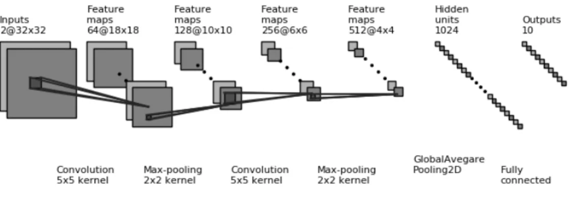
Since [38], the CNN’s have been dominating the field of computer vision. This con-tinuous progress has resulted in several types of architecture’s for CNN which include, VGG[39]), ResNet[40] and Inception Networks[41]. The advent of the regularization al-gorithms like Batchnormalization[42], Dropout[43] and optimization algorithms including adam[44], and RmsProp has enabled to train deeper architectures with millions of param-eters. The sample architecture of the convolutional neural networks is shown in the figure 2.12.
In general, all the convolutional neural network architectures consists of the following layers.
Figure 2.12: Two channel Convolutional Neural Network Architecture for audio classifica-tion
2.4.1
Convolutional layer
Convolutional layer, in short, Conv layer consists of a set of four-dimensional filters. The first and second dimension of the filter corresponds to height and width of the filter, fol-lowed by the third dimension representing the number of channels of the input, and the fourth dimension corresponds to the number of filters employed. Conv layer performs a mathematical operation called convolution, hence its name, between the input tensor and the set of filters. The convolution operation involves flipping the filters by 180◦and sum-ming the result of element-wise product between the flipped filters and the input tensor. However, unlike the fields of mathematics and signal processing, the convolution opera-tion performed in the scope of CNN does not involve kernel flipping, and strictly speaking, this operation is called cross-correlation. However, in CNN literature it is interpreted as convolution operation since the filters are capable of learning weights when filters are not flipped relative to the case where the filters are flipped. The sample convolution operation performed on single-channel input and a single channel filter is shown in figure 2.13. The filters in CNN are also called kernels. The hyper parameters that control the shape of the output volume of the layers in the CNN are padding, stride and depth.
Stride
Stride is represented by a integral number which interprets the amount of shift the kernel is eligible to make across both the height and width dimension of the input in calculating the output feature map of the convolutional layer.
Padding
Padding is defined as the addition of the dummy pixels around the input of a convolutional layers, usually to preserve the dimensions of the input tensor corresponding to the output feature map. The common forms of padding are zero padding and the reflection padding.
Depth
The depth of the output volume of a convolution layer is defined by the number of filters applied on the input tensor.
Let nHprev, nWprev and nC be the height, width and the depth of the input image,
f, f, nprev, nC be the height, width, the depth of the input, which defines the shape of the filter andfis the number of filters applied. WithnH, nW andnC as the dimensions of the output volume of a convolutional layer with a stride ’s’ and padding ’p’ the output of the Convolutional layer is given by
nH = [ nHprev −f+ 2∗p s ] + 1 (2.8) nW = [ nWprev −f+ 2∗p s ] + 1 (2.9)
Figure 2.13: Convolution operation in CNN
2.4.2
Activation Layer
The activation layers employees activation function over individual entities of a feature map. This transforms the input from linear hypothesis space to non-linear hypothesis space. Commonly used activation functions include Rectified Linear Units(ReLU), Exponential Linear Units(ELU), sigmoid and Softmax. The dimensions of the input and output tensor of an activation layer are the same.
2.4.3
Pooling Layer
Along with the activation layer, Pooling layer is a non-parametric layer in the CNN; it is employed to reduce the dimensions of the input tensor and to make the network insensitive to the small changes in the data due to noise. The most common types of Pooling operations are Maximum Pooling which yields the maximum value in the analysis window to the
output tensor, and Average Pooling which yields the average of all individual values in the analysis window to the output tensor. The presence of the Pooling layers is responsible for the CNN’s property of translational invariance. The sample pooling operation performed with a pool size of 2 and a stride of 2 is shown in figure 2.14.
LetnHprev, nWprev and nCprev be the height, width and the depth of the input to the Pooling layer, with stride s the output volume of the Pooling is defined by the following.
nH = [ nHprev −f s ] + 1 (2.11) nW = [ nWprev −f s ] + 1 (2.12) nC =nCprev (2.13)
2.4.4
Dense Layers
Dense layers are employed in the last layers of the CNN, which are similar to the fully con-nected Feed Forward Neural Network. The convolutional and pooling layers act identically to the sensory organs of the human body generating a hierarchical representation of input features, which are later fed into the Dense layers. The Dense layers take this represen-tation as the input and act like a regular ANN classifier with no shareable parameters and dense connections. The last Dense layer of the CNN outputs the class probabilities.
The back-propagation of error gradients in convolutional neural networks are found in [45]
2.5
Hyper Parameters
The model parameters defined by the user before the beginning of the training, which is capable of determining the capacity and the complexity of the model are defined as hyper-parameters. And once set, their values remain constant. The process of choosing the values for these parameters to increase the performance of the model over a series of training loops is called hyper-parameter tuning. In the recent decade, several algorithmic and regularization techniques were proposed, which resulted in a significant increase in the performance of the models. The hyper-parameters employed in the scope of this thesis work are as follows.
2.5.1
Gradient Descent:
The core idea of training a supervised learning model is to approximate a function which maps the input feature vector to the labeled output, which can later be used for inference. Gradient Descent is defined as an algorithmic technique employed to update the parameters of a function such that it minimizes the difference between the function output and desired
output. It is achieved by iteratively moving towards the lowest point on the error surface by the direction provided by the negative of the gradient.
WithJ(θ)as the hypothesis function,αas the learning rate, andOθJ(θ)as the gradient of the hypothesis function three variants of implementation schemes exists for Gradient Descent depending on the number of samples used to update the function parameters, which are described in the following subsections.
Stochastic Gradient Descent(SGD)
In SGD the error is calculated after performing the forward propagation of each sample, and the function parameters are updated. The advantages of SGD include faster compu-tation for more massive datasets and faster convergence since the function parameters are frequently updated. However, frequent updates result in high noise during training and high variance[46] in the gradient. The mathematical equation to perform SGD is as follows
θ:=θ−α.OθJ(θ;x(i);y(i)) (2.14)
Batch Gradient Descent
In Batch Gradient Descent the function parameters are updated only after calculating the error for the entire dataset. It is computationally faster with the datasets of reasonable size, has a stable convergence with minimal variance in gradient. However, usually, it doesn’t reach the optimal convergence and keeps oscillating around the optimal convergence point. The mathematical equation to perform Batch Gradient Descent is as follows.
Mini-Batch Gradient Descent
It is the most used variant of the Gradient Descent algorithm, which leverages the advan-tages of both Stochastic and Mini-Batch Gradient Descent. In this, the function parameters are updated after calculating the error for ’N’ number of samples usually called mini-batch. Here, the mini-batch size ’N’ is also a hyper-parameter, which is chosen by the user. The mathematical equation to perform Mini-Batch Gradient Descent is as follows.
θ:=θ−α.OθJ(θ;x(i:i+N);y(i:i+N)) (2.16)
2.5.2
Optimizing Gradient Descent
The recent research in Deep Learning also resulted in algorithmic techniques, to further optimize the gradient descent. The optimizers used in the scope of this thesis work are shown in the following paragraphs.
Learning Rate It is the hyper-parameter with the highest precedence in training the su-pervised learning neural network models. It is denoted by α. The negative gradient
ob-tained on the hypothesis function is scaled by the learning rate and is added to the pa-rameter as an update. Higher values of learning rate rise the problem of overshooting the optimal point or global minimum in the error surface of the hypothesis function, while the lower values of the learning rates results are convergence time by many folds. There exists no right value for choosing the correct value for the learning rate parameter and should be selected by examining the performance of the model by varying it. Several techniques like cyclic learning rates [47], stochastic gradient descent with warm restarts[48], and differen-tial learning rates have shown a significant increase in performance of the neural networks.
ror surfaces. When naive SGD approaches ravines caused by local minima, it takes a very wavering update increasing the convergence time. Momentum is a term added during parameter update which enables us to increases the size of the steps taken in parameter updates when the gradient points in the same direction decreasing the convergence time, also, yields smoother variations in the case when the gradient is changing its direction frequently. Momentum also enables the error function to jump over the local minima and reach global minimum. Withvtandvt−1as the gradient of the current and the previous step
respectively, andβ as the momentum the equations for Gradient Descent with momentum
are as follows.
vt=β1vt−1dθ+ (1−β1)dθ (2.17)
θ :=θ−α.vt (2.18)
(a) Ideal Convex Error Surface (b) Real Convex Error Surface
Figure 2.15: Convex Error Surface
gradients for that weight. Withstandst−1 as the exponential average of the squares of the
gradients, in current and previous time step and β as the decay parameter whose value is
usually chosen to be 0.9, the equations for RMSprop optimizer are.
st=β2st−1+ (1−β2)f 0 (θt)2 (2.19) vt+1 = α √ st f0(θt) (2.20) θt+1 :=θt−vt+1 (2.21)
Adam Adaptive Moment EstimationAdam [43] is an advanced stochastic optimization algorithm employed to update the trainable parameters of the model which combines the best of both momentum and RMSprop. It is reported that in practice this results in better performance compared to the existing optimizer algorithms for a large variety of problems. Also, Adam has the least convergence time among the Gradient Decent optimizers. With
vtas the exponential average of gradient andstas the exponential average of squares of the gradients, the equations for the Adam optimizer are.
vt =β1∗vt−1−(1−β1)∗f 0 (θt) (2.22) st=β2∗st−1 −(1−β2)∗f 0 (θt)2 (2.23)
While computing the first and second moment estimates, the initial values are computed by considering an arbitrary value v0. Which results in bias towards v0 while computing
the initial steps of the exponentially weighted moving averages. This can be overcomed by performing bias correction. The equations to perform the bias correction on both the first moment estimatevtand the second moment estimatestare as follows.
scorrectedt = st 1−βt 2 (2.25) θ:=θ−α v corrected t p scorrected t + (2.26)
The detail overview of the performance of the optimization of gradient descent algo-rithms are found in [51]
2.5.3
Regularization techniques
Dropout Dropout is a regularization technique first introduced by, which prevents the neural network from overfitting to the training set. In this technique, for each epoch, the network randomly drops the connections between the current layer and the next layer with a probability ’P.’ Dropout layers are not used during inference, and the weights are multiplied with the probability ’P.’
Gaussian Noise Gaussian Noise is defined as statistical noise, generally added to the in-put feature vector to reduce the variance during training. The Probability Density Function of a Gaussian Noise is Gaussian. Hence it’s named.
Batch Normalization Batch normalization also serves as a regularization technique is used to reduce the internal co-variance shift in the network and accelerate the training of neural nets. The equationa for batch-normalziation can be found in the figure 2.16.
2.5.4
Initializtion and Transformation Hyper-Parameters
Weight Initialization In training deep neural networks, for a long time, we had dealt with the problem of vanishing gradients and exploding gradients. Recent advances in the deep learning have resulted in different kinds of weights initialization techniques which
Figure 2.16: Equations for Batch-Normalization[42]
In the scope of this thesis work the glorot uniform or Xavier uniform initializer[52] is used to initialize all the weights in the network. Withn[L−1]representing the number of
neuron inL−1layer andn[L]denotes the number of neurons inLthlayer, the variance of initialization of the function parameters are as follows.
var(θi) =
2
n[L−1]+n[L] (2.27)
Activation Functions As discussed earlier the core idea of Neural Networks algorithms is to approximate function in the given hypothesis space. However, irrespective of the depth of the architecture, neural networks with no activation, performs linear transformations to the input which results in a linear relationship between the input and output. The linear hypothesis space is highly limited and results in poor performance. Activation function transforms the input from linear hypothesis space into non-linear hypothesis space, result-ing in significant improvement in performance. The activation functions used in the scope
of this thesis work include Rectified Linear Unit(ReLU), sigmoid, softmax and Exponential Linear Unit(’ELU’).
Figure 2.17: Activation Functions.
2.6
Principal Component Analysis
Principal Component Analysis[53] is a linear dimensionality reduction and visualization technique, used to map high-dimensional data with co-related features onto lower-dimensional space with uncorrelated features. This is achieved by calculating the new axes called princi-pal components, such that the first few principrinci-pal components retain the maximum variance existing in the original higher-dimensional space. In layman’s terms, principal components are the directions in the Dataset with the highest variance.
The steps involved in performing the principal component analysis are as follows. 1) Pre-processing the dataset.
variance matrix.
4) Feature selection or Selecting the transformed features.
Preprocessing the dataset The Dataset needs to be normalized before performing PCA. The core idea of PCA is to map the original Dataset on to directions which maximize the variance. In the case of the unnormalized Dataset, if there exist some features with large variance and some with small variance, PCA is biased towards the features with the large variance, and the calculation of the principal components is dominated by such feature. Normalizing the Dataset by making each feature to stay on the same range will overcome this phenomenon.
Calculating the co-variance matrix Co-variance measures the strength of the relation-ship between two random variables. A positive covariance value represents that both the variables increase or decrease together, while negative value represents an inverse relation-ship between the two variables such that the increase or decrease in one variable results in decrease or increase in the value of the second feature, followed by zero co-variance represents two mutually independent variables.
cov(x, y) =
PN
i=1(xi−x¯)(yi−y¯)
N −1 (2.28)
Since covariance measures the strength of the relationship between two random vari-ables when there exists more than two features or dimensions in the Dataset, the covariance matrix is calculated. For example consider a dataset with features x, y, and z, now the co-variance values are computed between x, y and, y, z and x, z. The co-co-variance calculation in commutative that is the co-variance between x, y, and y, x are equal. The covariance matrix is symmetrical across the diagonal with the diagonal representing the variances, which is the covariance of the variable with itself. A sample covariance matrix with the features x,
y and z is shown down below C =
cov(x, x) cov(x, y) cov(x, z)
cov(y, x) cov(y, y) cov(y, z)
cov(z, x) cov(z, y) cov(z, z)
(2.29)
In some instances, the correlation matrix is employed as an alternative to the covari-ance matrix. The correlation matrix is obtained by normalizing the covaricovari-ance matrix by dividing it with the product of a standard deviation of the variables individually.
Performing Eigen Value Decomposition or Singular Value Decomposition Either of the Eigenvalue decomposition or Singular value decomposition is performed on the Co-variance matrix to calculate the principal components. The eigenvectors corresponding to higher eigenvalue represents the stronger co-relation, while the eigenvectors corresponding to the lower eigenvalues represents weaker co-relation.
Feature selection or selecting the transformed features After calculating the principal components of the dataset, we have a choice of choosing then features contributing most to the calculation of the first few principal components in various combinations or can select the transformed features(principal components) as the new set of features for further processing
2.7
Random Forest Algorithm
Random Forests[54] algorithm, first proposed by Breiman in 2001, belongs to a class of ensemble methods employed for both classification and regression tasks. The random forest consists of a random combination of learning models called decision trees. This bagging
Similar to PCA, a random forest is also used to analyze the relative importance of the features in the dataset. When dealing with high dimensional datasets, in general, it is observed that there exists a fewer number of features which contribute to the accurate final prediction, while the other features add noise into the training algorithm and result in overfitting problem. The top ’N’ features with higher relative importance can be selected and employed with better algorithms for further improvement in prediction accuracy.
As stated earlier, random forests are a collection of decision trees. However, there exist some critical differences between them. In random forest algorithm, each decision tree is built considering partial dataset and the arbitrary number of features; the final prediction is performed by taking a vote on the results obtained by all the decision trees in the random forest. However, decision trees are built on entire dataset resulting in significant amount of over-fitting problem.
2.8
Libraries
2.8.1
Kapre
Kapre [55] is a keras extension layer that could be placed as a part of the keras model. The feature extraction techniques like Spectrogram, Melspectrogram exists as a layer class which can be placed as a part of the keras model. Kapre layers allows to extract features on the fly on top of gpu.
2.8.2
librosa
Feature extraction for convolutional neural networks and visualization is done using the python package librosa [56].
2.8.3
openSMILE
Deep learning algorithms are hungry for data, The lack of availability of the data in the field of environmental sound classification, to some extent can be supplemented with in-creasing the dimensionality of the input data space, and this is achieved by using large feature extraction libraries like open Source Media Interpretation by Large feature Extrac-tion (openSMILE). openSMILE was written in ’C’ language and has support for live audio supported with Portaudio and openCV. Writing the custom configuration files in this envi-ronment lets us to extract a large hand engineered feature vector of a signal, and the data is stored in a CSV file. In one of the top performing model for DCASE task1a, a 6552dimen-sional feature vector was used to enhance the performance on a Deep neural network.
The feature extraction on an audio signal can be performed in three levels, in the first level, the features can be extracted from any point in the signal and are called instanta-neous descriptors, followed by segmenting the signal into smaller frames of given size and extracting the features in the segmented regions or frames, and extracting features describ-ing the relation between the features computed on multiple frames.
The following explains the various levels of audio feature extraction provided by the openSMILE library.
Low-Level audio descriptors(LLD’s) Low-Level audio descriptors are computed by in-spection of the audio signal, which represents the signal itself in various domains. The various domains in which the LLD’s are calculated include
1) Temporal Descriptors 2) Spectral descriptors 3) Cepstral descriptors and 4) Perceptual descriptors
Delta Regression Coefficients In calculating the Low-Level Descriptors, the features are extracted from various points in the signal, and these features do not interact with each other. Delta-Regression coefficients are computed on LLD’s as a post-processing step to calculate the relation between the features over frames. This gives a better understanding of the signal and also increases the model performance.
δlw(n) = PN i=1i∗(x(n+i)−x(n−i)) 2∗Pw i=1i2 (2.30)
Functionals: To perform the tasks of Automatic Speech Recognition, Music Genre Clas-sification, human emotion clasClas-sification, and Acoustic Scene ClasClas-sification, the instanta-neous features of the signal and the relation between them over frames are not sufficient. These tasks need to look into long-term dependencies, for example, to classify an acoustic scene the model needs to initially compute all the events happening in the scene, followed by identifying the relationship between those events to make the final prediction. To do this, statistical, polynomial, regression and transformations functionals are applied to the low-level features.
SMILE988 Features Extraction:
Emo base[58] configuration file was employed to extract 988 features for each sample. The extracted features include 26 low-level descriptors (LLD) which contain 12 MFCC’s, 8 line spectral frequencies, F0 envelope, Intensity, Loudness, Pitch, probability of
voic-ing, Zero-crossing rate. The low-level descriptors are used to compute 26 Delta regression coefficients followed by applying 19 functionals which include Max./Min. value of respec-tive relarespec-tive position within input, range, arithmetic mean, 2 linear regression coefficients and linear and quadratic error, standard deviation, skewness, kurtosis, quartile 1-3, and 3 inter-quartile ranges to low-level descriptors and Delta regression coefficients.
Feature Group Description
Waveform Zero-Crossings, Extremes, DC Signal energy Root Mean-Square & logarithmic
Loudness Intensity & approx.loudness FFT spectrum Phase, magnitude(lin, dB, dBA) ACF, Cepstrum Autocorrelation and Cepstrum
Mel/Bark spectr. Bands 0-N mel
Semitone spectr. FFT based and filter based Cepstral Cepstral features, e.g.MFCC,PLPCC
Pitch F 0 via ACF and SHS methods Voice Quality HNR, Jitter, Shimmer
LPC LPC coeff., reflect. coeff., residual Line spectral pairs(LSP) Auditory Auditory spectra and PLP coeff.
Formants Centre frequencies and bandwidths Spectral
Energy in N user-defined bands, multiple roll-off points, centroid,entropy, flux, and rel. pos. of max./min. Tonal CHROMA, CENS, CHROMA-based features
Table 2.3: [57] openSMILE’s low-level descriptors
Category Description
Extremes Extreme values, positions, and ranges Means Arithmetic, quadratic, geometric Moments Std. dev., variance, kurtosis, skewness Percentiles Percentiles and percentile ranges Regression
Linear and quad. approximation coefficients, regression err., and centroid
Peaks Number of peaks, mean peak distance, mean peak amplitude Segments
Number of segments based on delta thresholding, andmean segment length
Sample values Values of the contour at configurable relative positions Times/durations Up- and down-level times, rise/fall times, duration Onsets Number of onsets, relative position of first/last on-/offset DCT Coefficients of the Discrete Cosine Transformation(DCT) Zero-crossings Zero-crossing rate, Mean-crossing rate
Table 2.4: [57] Functionals(Statistical, polynomial regression, and transformations) avail-able in openSMILE
SMILE6k Feature Extraction:
Emo large[59] configuration file was employed to extract 6552 features for each audio sample. This is the full scale extraction of features supported by openSMILE. The features include 56 low-level descriptors (LLD), 56 Delta regression features computed on LLD’s and 39 functionals are applied on LLD’S and Delta Regression features.
The detailed description on the features extracted from the openSMILE library can be found in the chapter 2 of the document [60].
3 Performance Measures
There exists numerous performance metrics in the current machine learning literature. Defining the right metric is one of the crucial steps in defining the solution to the lem. The choice of the performance metric depends on various things which include, prob-lem definition, the distribution of the classes in the dataset, and the trade-offs that we are consciously willing to make to yield an effective solution to the defined problem. The met-rics employed in the scope of this thesis work include classification accuracy, precision, recall, Receiver Operating Characteristic curve, precision-Recall curves, and F1-score for multi-class with micro, macro, and weighted averages.
The naive approach to evaluating the performance of an binary or multi-class classifier is to calculate the classification accuracy. With P as number of correct predictions and N as the total number of samples in the dataset, classification accuracy is given by the ratio of P to N.
classif ication accuracy = N umber of correct predictions(P)
N umber of samples in the dataset(N) (3.1)
Class wise classif ication accuracy = N umber of predictions of class(p)
Actual Class Predicted Class Back-Ground Single Drone Two Drone T w o Drone Single Drone Back-Ground 100 0 0 0 565 35 0 51 49
Figure 3.1: Sample Confusion Matrix for multi-class classification
3.1
Confusion Matrix
The first step involved in the calculation of advanced performance metrics is to compute the confusion matrix. The confusion matrix consists of actual values on one dimension and predicted labels on the second dimension with each class consisting of a row and column. The diagonal elements of the matrix represents the correctly classified samples. The sample classification matrix for the multiple drone detection problem is shown in the figure 3.1.
The metrics that can be computed from the confusion matrix include Precision, Recall, F1-score which is the harmonic mean of the precision and recall, and the classification accuracy.
To build intuition on the metrics precision and recall, consider a binary classification problem with class-0 and class-1 corresponding to background noise and single drone in the scene.
Precision: It is defined as how many of our predicted samples with a drone in the scene actually contains the drone.
Recall: It is defined as the fraction of number of samples predicted to have a drone in the scene to the number of samples actually has drone in the scene.
F-Measure It is defined as the harmonic mean between the precisi